Fluorescence and Multiphoton Imaging for Tissue Characterization of a Model of Post-Menopausal Ovarian Cancer

Abstract

Objectives:

To determine the efficacy of targeted fluorescent biomarkers and multiphoton imaging to characterize early changes in ovarian tissue with the onset of cancer.

Methods:

A transgenic TgMISIIR-TAg mouse was used as an animal model for ovarian cancer. Mice were injected with fluorescent dyes to bind to the folate receptor α, matrix metalloproteinases, and integrins. Half of the mice were treated with 4-vinylcyclohexene diepoxide to simulate menopause. Widefield fluorescence imaging and multiphoton imaging of the ovaries and oviducts was conducted at four and eight weeks of age. The fluorescence signal magnitude was quantified, and texture features were derived from multiphoton imaging. Linear discriminant analysis was then used to classify mouse groups.

Results:

Imaging features from both fluorescence imaging and multiphoton imaging show significant changes (p<0.01) with age, VCD treatment, and genotype. The classification model is able to classify different groups to accuracies of 75.53%, 69.53%, and 86.76%, for age, VCD treatment, and genotype respectively. Building a classification model using features from multiple modalities shows marked improvement over individual modalities.

Conclusions:

This study demonstrates that using widefield fluorescence imaging with targeted biomarkers, and multiphoton imaging with endogenous contrast shows promise for detecting early changes in ovarian tissue with the onset of cancer. The results indicate that multimodal imaging can provide higher sensitivity for classifying tissue types than using single modalities alone.

Introduction

Ovarian Cancer

Ovarian cancer is a devastating disease with high mortality rates because non-specific symptoms and lack of an effective screening test leads to frequent late diagnosis. In the U.S. alone there are more than 20,000 new cases of ovarian cancer each year and approximately 14,000 deaths per year [1]. However, if ovarian cancer is found and treated before metastasis, the 5-year survival rate is 94% (versus 28% for metastatic disease) [1, 2]. Unfortunately, no reliable early detection technique exists [3]. Owing to the challenges associated with early disease detection, there is limited data available on women. Animal models can provide needed information that will help develop an understanding of early cancerous changes and lead to future development of screening tests for women that are at high risk for developing ovarian cancer.

The most common type of ovarian malignancy is derived from epithelial cells and is more likely to occur in post-menopausal women. In addition, recent studies have shown that some ovarian cancers may originate in the fallopian tubes[4]. Thus, both the ovaries and fallopian tubes may exhibit early tissue changes with the onset of cancer.

In this study we combine a menopausal mouse model and transgenic ovarian cancer model and characterize ovarian and fallopian tube tissues in these models using optical imaging techniques. The information on tissue changes observed in these models will be helpful for future studies examining neoplastic and cancerous changes. We find that using structural and functional imaging techniques such as multiphoton microscopy and widefield fluorescence imaging, it is possible to detect changes in ovarian tissue.

Imaging Modalities

Optical imaging methods are excellent for visualizing tissue changes due to the high resolution and high sensitivity to tissue changes. Due to the abundance of different modalities, optical imaging enables the flexibility of imaging scales from wide field to narrow field (higher resolution) as well as imaging either endogenous or exogenous contrast sources, including fluorophores and scatterers. Tissue fluorophores absorb incident light and subsequently emit light, generally of a longer wavelength. The wavelengths and intensity of the remitted light are related to the quantity, type, and distribution of fluorophores present.

Optical imaging techniques that have shown promise for detection of ovarian cancer include fluorescence imaging [5], multispectral imaging [6], confocal imaging [7], multiphoton microscopy [8, 9], photoacoustic imaging (PAI) [10], and optical coherence tomography (OCT) [11], among others. Reflectance and fluorescence spectroscopy can differentiate normal and neoplastic ovarian tissue but typically has poor resolution [12]. OCT visualizes details of tissue microstructure such as surface epithelium, follicles, cysts, collagen bundles, and vessels as well as potentially abnormal changes such as invaginations and changes in tissue density, but has inadequate resolution for cellular changes [13, 14]. Confocal microscopy produces subcellular-resolution images that can be used to identify cancer occurring on the surface of the ovary, but the depth of imaging is limited [7, 15]. PAI has the largest depth of imaging (2 to 3 cm) and, owing to differences in absorption properties, can visualize large structures such as corpora lutea, follicles, and blood vessels [16, 17]. Likewise, malignant and normal ovaries in postmenopausal women can be distinguished by their different absorption properties. However, PAI has relatively low resolution and may be confounded by benign conditions with high vascularity or hemorrhage, or early-stage cancers without significant vascularity changes [18].

Since each of these modalities has limitations of resolution, field of view, and use different contrast mechanisms to provide sensitivity and specificity to different markers of early disease, we propose to use multiple modalities, specifically, widefield fluorescence imaging and multiphoton microscopy, to get both large field of view and high resolution. Furthermore, these techniques enable visualization of exogenous and endogenous fluorophores, respectively.

Widefield Fluorescence Imaging and Dye Selection.

Widefield fluorescence imaging (WFI) illuminates a large area of tissue, so that high resolution information from entire organs can be viewed quickly, with little or no scanning. In the case of a mouse, we are able to view the entire reproductive tract including uterus, oviducts (murine equivalent of fallopian tubes), and ovaries in a single image. The addition of targeted fluorescent dyes can provide both qualitative and quantitative information on desired markers in the tissue and overall tissue composition. A number of different light sources and filters can be used to separate the excitation and emission of fluorophores of interest.

A number of commercial fluorescent dyes are available for tissue characterization. We are most interested in tissue markers that are potentially upregulated in cancer so that we can understand the expression of these markers in the mouse models that we use. The tissue markers that were of highest interest to us and commercially available included folic acid, matrix metalloproteinases and integrins.

Folic acid is an essential nutrient required by all living cells for cellular division. Uptake of folic acid is necessary for the metabolism of tumor cells. Folate receptor alpha (FR-α) is a protein that uptakes folic acid by endocytosis and can be over-expressed in ovarian epithelial cancers [19, 20]. Little to no folate receptor expression was found in nonepithelial tumors and in normal tissues, while significantly higher expression was found in ovarian carcinomas [21]. FR-α promotes growth of tumors by its modulation of folate uptake or regulatory signals [22]. The expression of FR-α is normally restricted to certain tissues where the receptor does not come in direct contact with the circulating folate [22]. In cancerous tissues, FR-α is available to circulating folate. It is suggested that the expression FR-α is regulated by estrogen receptor (ER) expression in tumors. The expression of elevated estrogen receptors in gynecological malignancies such as cervical and ovarian cancer cell lines is suggested to repress the expression of FR-α [23]. The activation of FR-α is associated with the activation of signaling pathways that induce oncogenic transformation, such as the activation of oncogene signal transducer and activator of transcription 3 (i.e., STAT3) that can promote growth, proliferation, and survival of cancerous cells [24].

Matrix metalloproteinases (MMPs) also have an important role in ovarian malignancies. MMPs interact with component of the extracellular matrix to carry out tissue remodeling pathways [25]. During ovulation, the extracellular matrix is degraded; MMPs mediate the breakdown of the basement membrane which is required for the release of the oocyte. Certain MMPs also help in the atresia process. There are approximately twenty-three members in the MMP family and they are grouped based on their function and structure. Increased expression of MMP2 and MMP9 was found in epithelial ovarian cancer cell lines, significantly higher expression was found in advanced cancer stages [26]. Previous studies have also indicated that MMP-2 and MMP-9 can be overexpressed early in cancer progression of human ovarian carcinomas. It is suggested that there is a difference in expression of mRNA levels of MMP-9 in samples of normal ovaries and polycystic ovaries of postmenopausal women. Lower levels of MMP-9 mRNA were found in normal ovaries of postmenopausal women in comparison to polycystic ovaries [27]. MMP-9 and MMP-2 expression in ovarian cancer relates to the ability of cancer cells to invade and metastasize [28, 29]. Silencing of MMP-9 decreased the ability of cancer cells to invade [26]. One of the main pathways that is altered by MMPs in cancer cells is the tumor growth factor (TGF) - β signaling pathway, which is known to be activated both MMP-2 and MMP-9. Altered expression levels of MMPs are known to affect the activity of other MMPs, growth factors, cytokines and epidermal growth factor (EGF) that induce oncogenic transformation of cells [30].

Integrins are cell surface receptor proteins that regulate signal transduction between cells and the extracellular matrix. These receptor proteins are composed of two subunits, the α subunit and the β subunit. The two subunits can combine to create twenty-four integrin receptors [31]. Integrins play an important role in integrating the extracellular matrix and the cytoskeleton of cells. Overall, integrins have been known to be interrelated with metastasis [32]. One integrin known to be associated with cancer cell lines is α_νβ₃. Integrin α_νβ₃ can be upregulated in tumor cells and is associated with survival and angiogenesis [33, 34]. The expression of integrin is found to be associated with epithelial cadherin (E-cadherin). E-cadherin is an important adhesion molecule that forms cellular junction and is expressed in epithelial cells. Elevated levels of E-cadherin expressed in ovarian cancer cell lines were silenced to test its effects on the integrin expression. It was found that loss of E-cadherin up regulates α_ν integrin expression [35]. The resulting elevated levels ofα_ν integrin, due to loss or down-regulation of E-cadherin, play a role in the activation of signaling pathways involved in adhesion and metastasis [35]. The ability of cancer cells to establish themselves in distant sites is largely regulated by integrins. Integrins of ovarian cancer cell lines mediate the adhesion to fibronectin, laminin and collagen which aid in further invasion and tumor growth [36].

Multiphoton Microscopy.

In multiphoton microscopy (MPM), femtosecond pulsed laser light is focused with high numerical aperture optics to create a high instantaneous power density in a small volume of tissue, enabling multiphoton events that result in submicron resolution imaging with little out of focus signal generation. MPM using near-infrared light has the ability to image the same fluorophores hundreds of microns deeper than confocal microscopy using ultraviolet or visible light. The laser is scanned in two dimensions while the sample is moved in the third dimension to create a 3-D image set. In two-photon excited fluorescence (2PEF), two photons are simultaneously absorbed by a fluorophore and then emitted as one photon at a higher frequency than the incident light. Using excitation light near 800 nm, endogenous fluorophores that can be visualized with 2PEF include proteins containing aromatic amino acids (tryptophan, tyrosine, phenylalanine), metabolic co-factors such as NADH and FAD, structural proteins such as collagen and elastin, and a variety of other molecules including vitamins and lipopigments [37, 38]. In second harmonic generation (SHG), phase matching of photons in non-centrosymmetric structures results in a scattering event in which two photons are combined into a single photon at twice the frequency of the incident light [39]. SHG is primarily used for visualization of collagen. Light collected from 2PEF and SHG are separated using bandpass filters. MPM enables visualization of changes in endogenous cellular fluorescence and collagen structure resulting from ovarian tissue changes, including cancer. Likewise, SHG enables visualization of changes in collagen fibers resulting from ovarian tissue changes.

Animal Model.

The syngeneic TgMISIIR-TAg (TAg) mouse [40, 41] expresses the transforming region of polyomavirus simian virus 40 (i.e., SV40) under control of the Mullerian inhibitory substance type II receptor gene promoter, which is expressed in ovarian epithelial cells, including fallopian tube and endometrium [42]. All TAg positive (TAg+) TgMISIIR-TAg female mice develop bilateral epithelial ovarian cancer, with invasive tumors in the ovaries evident in nearly all mice by 8 weeks of age [43].

Repeated exposure to the chemical 4-vinylcyclohexene diepoxide (VCD) has been shown to accelerate the rate of atresia in small follicles in the ovaries of rats and mice and lead to early ovarian failure [44, 45, 46]. Thus, VCD has been useful for generating an animal model for menopause, even in young animals. In a previous study we have shown that VCD dosing will cause ovarian failure in TAg+ mice and their non syngeneic counterparts.

Materials and Methods

Animals

All experiments were performed per NIH guidelines, and protocols were approved by the University of Arizona Institutional Animal Care and Use Committee. C57Bl/6 wild type (WT) female breeder mice 8 weeks of age were purchased from Jackson Laboratory. Six initial TAg+ males were obtained from the Fox Chase Cancer Center to start the colony. Animals were housed in microisolators per NIH guidelines and allowed a 7-day acclimation period before initiating the experiment. One to three C57Bl/6 females were housed with one TAg+ male for mating. Pregnancy in females was determined by the presence of a copulatory plug. Pups were born on days 20 – 21 following mating. Pups were evaluated for sex, and tail tips were collected from females for genotyping at either the University of Arizona Genetics Core or TransnetXY. An average of 4 females/litter were obtained. Approximately one half the females carried the transgene (TAg+) and one half did not (WT).

Dosing

On post-natal day 7, dosing of females with sesame oil (S3547; Sigma Chemical Company, St. Louis MO), or sesame oil containing 80 mg/kg VCD (94956; Sigma Chemical Company, St. Louis MO), 2.5 ml/kg body weight, was administered by intraperitoneal injection. Daily dosing with sesame oil and VCD was continued for 15 days or 20 days.

Dye Application

Fluorescent imaging dyes included IntegriSense 680 (NEV10645; PerkinElmer, Waltham MA), FolateRSense 680 (NEV10040; PerkinElmer, Waltham MA) and MMPSense 680 (NEV10126; PerkinElmer, Waltham MA). Dyes were prepared according to package instructions and kept in foil wrapped tubes to protect from ambient light. Ovaries were surgically exposed in live animals as described below and a sterile pipette tip was used to place 50 uL of dye on to each ovary, or 100uL of dye into the body cavity (for control organs), resulting in a total of 100uL of dye per animals. Organs were allowed to incubate with dye for 10 minutes in darkness by turning off lights in the room and covering animal organs with an elevated black drape (not in contact with the animal). Following incubation, mice were euthanized by CO2 inhalation and organs were explanted.

Organ Explant and Tissue Processing

Entire reproductive tracts (including uterus, oviducts and ovaries) were explanted, thoroughly rinsed in saline, weighed, and placed on a non-reflective black pad for imaging. Widefield fluorescence imaging was performed first, followed by multiphoton imaging. Imaging was completed in approximately 30 minutes post-explant. Orientation was carefully maintained from explant to imaging, fixation, paraffin embedding, and sectioning, by maintaining anatomical orientation at explant and placing the reproductive tract ventral side up on filter paper indicating left-right and superior-inferior locations. After imaging, the tracts were fixed in 10% Buffered formalin solution for 20 – 24 hrs, transferred to 70% ethanol, dehydrated, embedded in paraffin blocks, and sectioned at 6μm thickness. Histology sections were taken parallel to the area imaged, allowing an enface view of the imaged area.

Table 1 summarizes the number of mice imaged and analyzed for MPM and WFI of fluorescent dyes. The same mice are imaged for both MPM and WFI, though some exhibiting image artifacts were excluded from analysis, as described in the following sections, which results in different totals between MPM and WFI.

TABLE 1.

Number of mice imaged and analyzed for multiphoton and widefield imaging of fluorescent dyes. The same mice are imaged for both MPM and WFI, though some exhibiting image artifacts were excluded from analysis (hence different totals). (4 - four weeks age, 8 - eight weeks age, W - wild type, T - TAg+, S - treated with vehicle sesame oil, V - treated with VCD).

	4WS	4TS	4WV	4TV	8WS	8TS	8WV	8TV
MPM Ovary	14	12	13	13	13	13	11	8
MPM Oviduct	14	12	13	13	13	13	11	8
MMPSense Ovary	8	8	5	7	12	9	5	5
MMPSense Oviduct	7	8	5	7	11	9	5	5
FolateRSense Ovary	5	5	5	5	6	8	5	5
FolateRSense Oviduct	5	5	5	5	6	8	5	5
Integrisense Ovary	5	6	5	5	5	5	5	5
Integrisense Oviduct	4	6	5	2	5	5	5	3

Widefield Fluorescence Imaging

Widefield fluorescence imaging (WFI) was performed with an MVX10 microscope with a DP80 digital camera (Olympus, Tokyo JP), and ImageX software. Images were taken at exposure times of 2 s (for MMPSense dye), 0.1 s (for FolateRSense), or 0.2 s (for Integrisense). Magnification was set to 0.8. Each channel was set to un-gated and a frequency of 100,000. Light was filtered using the microscope’s CY5.5 filter set, featuring a cut-on wavelength of 685 nm, excitation band of 635 – 675 nm and emission band of 696 – 736 nm. The excitation spectrum of these dyes does not overlap with the wavelength used for MPM, as described next; thus, there is no cross-interaction between fluorescence and MPM studies, as confirmed by examining both stained and unstained tissues with MPM.

Widefield Fluorescence Image Analysis

Images were examined by eye and excluded from analysis if saturation occurred. Based on prior pilot analysis the images with the best exposure times for each dye were selected to maximize the signal without observing saturation. Analysis was performed using ImageJ software [47]. For each organ, a 40×40 pixel square was placed in the center of the organ and the mean signal intensity in the region was recorded. This was done for both left and right ovaries and oviducts.

Multiphoton Imaging

MPM imaging was performed with a single-beam multiphoton microscope (TrimScope, LaVision BioTec, Bielefeld, GE) using a Titanium:Sapphire laser light source (Chameleon Ultra2, Coherent, UK) that was coupled to the scanner unit, with a pulse width of 120 femtoseconds at the sample. The laser intensity was adjusted to 35 mW average power with an electro-optical modulator (EOM 350–80; Conoptics, Danbury, CT). A water-immersion, coverslip-corrected, 20X magnification, 0.95-NA objective (MRD77200 Nikon, Tokyo JP) was used for imaging. The excitation wavelength was set to 780 nm, and SHG and 2PEF image data were recorded simultaneously. A bandpass filter (FF01–377/50; Semrock, Rochester NY) and a dichroic mirror (Di01-R405–25X36; Chroma, Bellows Falls, VT) were used to collect light for SHG and a bandpass filter (HQ450/100M-2p-25; Chroma) and a dichroic mirror (505dcxr; Chroma) were used to collect light for 2PEF. Images were taken at 5 μm depth increments from the surface of the tissue to 50 – 100 μm depth. Imaging was completed in less than five minutes per image stack Two image volumes were collected from two locations on the ovary. The first image value was approximately in the center of the ovary and the second was between the center of the ovary and the oviduct. Two image volumes were also collected from two separate locations the oviduct: the first near the ovary and the second farther away from the ovary. All images had a 400 μm × 400 μm field of view and contained 1024 × 1024 pixels with 14-bit gray scale resolution.

Multiphoton Image Analysis

Images were examined by eye and excluded from analysis if they had artifacts (e.g. debris, fur in the image) or had signal in less than approximately 50% of the image area. On the basis of visual examination of cellular and collagen features, it was expected that previously developed analysis algorithms using computation of spatial frequency content and standard gray-level co-occurrence matrix (GLCM) parameters and Fourier transform parameters may be able to quantify the tissue variations observed by eye.

Images were quantized to 8-bit before analysis. We applied two methods of texture analysis to extract features from the acquired MPM images. The first is based on constructing and analyzing the Grey-Level Co-occurrence Matrix (GLCM) [48]. The GLCM is a spatial histogram that describes the distribution of grey-level values in an image. Each entry in the GLCM, p(i, j|d, θ), corresponds to the probability of a pixel with a grey-level of (i) being a distance (d) pixels away from a neighboring pixel with a grey-level of (j) in the (θ) direction. With an image quantized into N_g grey levels, the GLCM is an N_g × N_g matrix. For a two-dimensional image, four directions for (θ) are possible: 0 degree, 45 degree, 90 degree, 135 degree. In this study, we fixed (d) at one pixel (3.9 μm in object space), and computed the GLCM for the four possible directions. All images were normalized and quantized to 8-bit (intensity ranging between 0 and 255). From the GLCM, we then computed thirteen texture features introduced by Haralick in 1973 [48], averaged over the four directions for θ.

We computed a second set of features by analyzing the discrete Fast Fourier transform (FFT) of the image in 2D, which describes the distribution of spatial frequencies present in an image. After applying the FFT, the image was normalized so that all pixel values summed to one. Then, we summed the pixel values in a small disk centered at the origin and recorded the result. The radius of this disk was iteratively increased and the summed pixel value within its area was recorded until the disk radius had reached 80% of the image half-width, beyond which primarily noise remains. This was effectively the cumulative distribution function (CDF) of the energy density as a function of radial spatial frequency; taking the difference between the values of this curve for any two radial frequencies gives the proportion of energy contained within a specific frequency band. Images that were highly homogenous had higher energy density associated with lower spatial frequencies. On the other hand, images with more inhomogeneity had more energy density corresponding to higher spatial frequency. We then parameterized the distribution by fitting the CDF curve to the following equation, which we qualitatively found to fit the curve well:

$$y=a{x}^b+c$$ (1)

Where y is the value of the CDF for a given spatial frequency x. The frequency distribution was thus described by the three features: a, b, and c, which were used to differentiate between the different experimental groups. Combining these with the thirteen Haralick features gave a set of sixteen texture features total. The analyses were completed in Python using a computer with an Intel Core I-4710HQ CPU (2.50 GHz) and 16 GB DDR3L memory.

Statistical Analysis

In this study, two types of statistical analyses were used to determine whether differences in imaging features could be observed between experimental groups. First, feature values between individual mouse groups were compared using a Student’s t-test. Equal variance was not assumed. For each experimental variable (age, treatment, genotype), four pairwise comparisons can be assessed, totaling twelve comparisons. Table 2 summarizes the different comparisons that are investigated for each variable.

TABLE 2.

Statistical significance is assessed for four comparisons for each experimental variable. Classification models are built for each of four comparisons within a variable. (4 - four weeks age, 8 - eight weeks age, W - wild type, T - TAg+, S - treated with vehicle sesame oil, V - treated with VCD).

	Age	Treatment	Genotype
Comparisons	4WS – 8WS	4WS – 4WV	4WS – 4TS
	4WV – 8WV	4TS – 4TV	4WV – 4TV
	4TS – 8TS	8WS – 8WV	8WS – 8TS
	4TV – 8TV	8TS – 8TV	8WV – 8TV

To adjust the analysis for the multiple comparisons, the Benjamini-Hochberg technique is applied [49]. For a given false discovery rate (FDR), the Benjamini-Hochberg critical value is calculated for each comparison and compared to the p-value to determine which comparisons are significant [50]. All twelve comparisons shown in Table 2 were considered to be part of a single family. Differences were considered statistically significant for an FDR of 0.1. For those features within this threshold, the significance is denoted on figures using the standard notation of p < 0.05 (denoted *), p < 0.01 (denoted **), p < 0.001 (denoted ***).

Next, a classification model is built to classify mice into separate groups using linear discriminant analysis. The same twelve comparisons shown in Table 2 are considered. For each, a separate classification model is built as described below. Ultimately, the classification performance is averaged for each variable to assess the overall ability of the imaging features to discriminate tissue for a given variable. Separate classifications are attempted using features produced from individual imaging modalities, as well as one attempt where all features are combined into a single set.

Feature Selection and Classification

Classifications were first attempted using five feature sets, each derived from a separate modality: two for SHG of the ovaries and oviducts, two for 2PEF of the ovaries and oviducts, and one for WFI both of the ovaries and oviducts. The features from both organs are combined in WFI since only two features are available. In addition, a classification was attempted using a feature set containing all features combined.

For each classification model using features from SHG or 2PEF, sixteen features are available to use in the classification model, as described above in Section 1. Two features are available for the WFI classification: mean signal for the ovaries, and mean signal for the oviducts. In addition, a classification model was built using a selection from all available features: the sixteen features from each of the four MPM modalities are combined with two features from WFI. In this case, the total number of features is 64.

For each feature set, the classification proceeded by first removing redundant by calculating the correlation matrix for the feature set. For each pair of features that were highly correlated (correlation > 0.85) [51, 52], one feature from the set was removed (the feature which yielded a lower average p-value using the statistical test described above).

We exhaustively tested the classification performance of feature subsets consisting of six or fewer features, as the literature suggests that high performance can typically be achieved with two to five features [51, 53, 54]. To evaluate how well a set of features could separate different classes, we used the trace of the ratio of the between-class scatter (S_b) and within-class scatter (S_w), which has successfully been applied in similar scenarios.

To classify the data, we used linear discriminant analysis [55], which has been applied frequently in the scope of medical image classification[56, 57, 11]. For our classification, we reduced the dimension to the number of linear discriminants that account for 99% of the variance in each case, before generating the optimal decision boundary. To validate the model, we used leave-one-out cross-validation. The accuracy for classifying based on age, genotype and treatment was calculated for all four possible comparisons for each variable (Table 2), and averaged to yield the final result. Additional details regarding our classification process have been previously described [11, 52].

Results

Widefield Fluorescence Imaging

Example images for WFI are shown in Fig. 1 for WT (a) and TAg+ (b) mice using MMPSense. It is visually apparent in these images that the fluorescence magnitude for TAg+ mouse ovaries and oviducts is significantly higher than WT. Results for quantifying the WFI signal in the ovaries and oviducts, along with analysis of differences between genotype are summarized in Fig. 2 for MMPSense (a) FolateRSense (c), and Integrisense (c). The results show that all three dyes significantly change in signal magnitude for eight week old mice dosed with sesame oil. In addition, MMPSense is significantly elevated for four-week VCD-dosed mice, and Integrisense is elevated for eight-week VCD-dosed mice. These results were observed for both ovaries and oviducts. A comprehensive comparison between individual experimental groups is summarized in Appendix 1.

Fig. 1.

Example images taken using MMPSense dye for wild type (a) and TAg+ (b) female mice at eight weeks dosed with sesame oil.

Fig. 2.

Signal intensity for widefield fluorescence imaging using MMPSense (a), FolateRSense (b), and Integrisense (c). (4 - four weeks age, 8 - eight weeks age, W - wild type, T - TAg+, S - treated with vehicle sesame oil, V - treated with VCD). Statistical significance is only denoted for comparisons between genotype groups. Differences were considered statistically significant for p < 0.05 (denoted *), p < 0.01 (denoted **), p < 0.001 (denoted ***).

Multiphoton Imaging

Fig. 3 shows composite MPM images for an ovary deep within the organ (a), and at a more superficial depth in the organ (b), as well as MPM images of an oviduct (c: deep, d: superficial). At different depths, the images show significantly different features, such as the organization of the collagen matrix (represented by SHG imaging in green in Fig. 3), as well as local metabolic activity and lipofuscin concentration (represented by 2PEF imaging in red).

Fig. 3.

Composite MPM images (green - SHG, red - 2PEF) for different depths for an eight-week wild type mouse. The ovaries deep (a), and superficial (b). The oviducts deep (c), and superficial (d).

Fig. 4 shows individual MPM images for a wild type and TAg+ mouse at eight weeks, dosed with sesame oil. Visually, the SHG images seem to exhibit a more disordered collagen structure in the TAg+ mice, which would be quantified with texture analysis. Furthermore, the 2PEF images, particularly those of the ovaries, seem to show local metabolic changes. The brighter signal could suggest enhanced metabolic activity, or may indicate increase accumulation of lipofuscin, which has been observed to increase both due to age and the presence of disease [8].

Fig. 4.

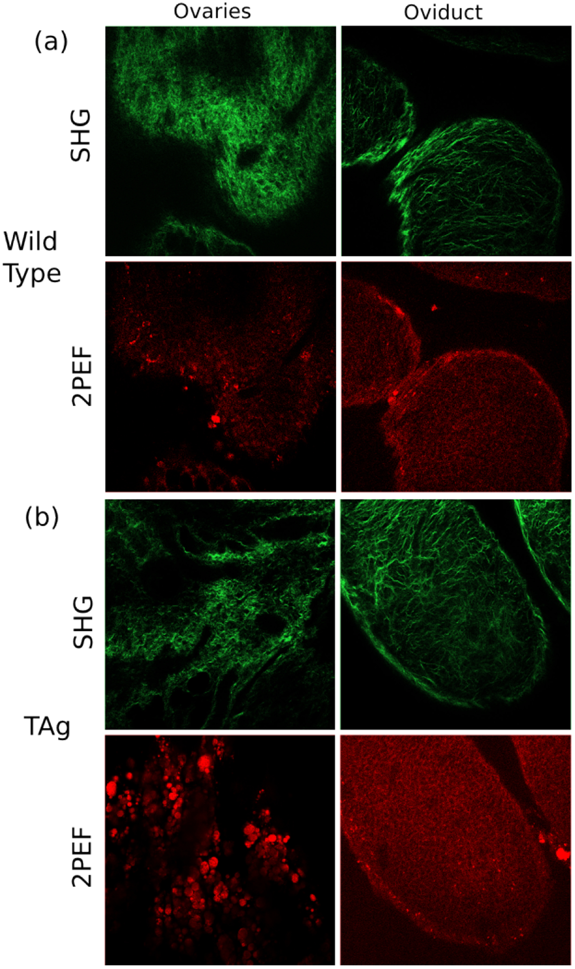
Sample SHG (top row) and 2PEF (bottom row) images for a wild type and TAg+ female mouse at eight weeks, both dosed with sesame oil.

The texture analysis results showed that many texture features were significant for comparisons between each variable. Table 3 summarizes the number of features for each modality that were significant for at least one comparison for each variable (see Table 2). Each MPM modality yielded an appreciable number of features that were significant for at least one comparison of each variable. Comparisons of tissue changes due to age yielded the highest number of significant features overall. SHG imaging of the oviducts was most sensitive to tissue changes caused by VCD treatment, with 10 features showing significance. 2PEF imaging of the oviducts also showed many features that were significant to the variable of VCD treatment. SHG imaging of the oviducts and 2PEF imaging of the ovaries yielded many features that showed significant differences between genotype groups. This may suggest that early tissue changes occur in the oviducts, primarily structurally, whereas early metabolic changes are observed in the ovaries, but the tissue microstructure is affected to a smaller degree. Appendix II includes a comprehensive list of feature values and standard deviations for each modality, categorized by mouse group.

TABLE 3.

Number of texture features for each MPM modality that are statistically significant for at least one comparison for each variable. The comparisons are listed in Table 2.

	Age	Treatment	Genotype
SHG Ovaries	6	4	4
2PEF Ovaries	7	3	6
SHG Oviducts	11	10	10
2PEF Oviducts	4	6	5

Fig. 5 shows an example texture feature’s ability to differentiate between genotype for SHG and 2PEF imaging of the ovaries and oviducts. There is a wide variety of features that show high statistical power, depending on which two experimental groups are of interest. In Fig. 5, statistical significance is only shown for genotype comparisons, as those are most clinically relevant.

Fig. 5.

One example texture feature chosen for each: (a) SHG ovaries, (b) SHG oviducts, (c) 2PEF ovaries, (d) 2PEF oviduct. (4 - four weeks age, 8 - eight weeks age, W - wild type, T - TAg+, S - treated with vehicle sesame oil, V - treated with VCD). Statistical significance is only denoted for comparisons between genotype groups. Differences were considered statistically significant for p < 0.05 (denoted *), p < 0.01 (denoted **), p < 0.001 (denoted ***).

Classification

Classification models were built for each comparison shown in Table 2, using features from SHG and 2PEF imaging of the ovaries and oviducts, as well as WFI imaging of both organs. Additionally, a classification model was built with all features combined into a single set. The classification results are summarized in Table 4 below, averaging across the four comparisons for each variable. Parenthesis in Table 4 represent the number of features used to build the model achieving the stated accuracy. We see that in no case is six features needed; four and five features is the most common. For the classification using all features, we see that four features yields the highest accuracy.

TABLE 4.

Classification results between experimental groups when using linear discriminant analysis. The number of features used to build the model for each case are shown in parenthesis next to the accuracy. Four comparisons exist for each variable. The results shown here are averaged over all four.

	Age	Treatment	Genotype
SHG Ovaries	0.711 (5)	0.614 (5)	0.572 (5)
2PEF Ovaries	0.718 (5)	0.728 (5)	0.503 (4)
SHG Oviducts	0.747 (5)	0.716 (5)	0.725 (4)
2PEF Oviducts	0.733 (5)	0.698 (5)	0.561 (4)
WFI	0.572 (2)	0.589 (2)	0.581 (2)
All Features	0.755 (4)	0.695 (4)	0.868 (4)

When combining all features into a single set, the highest classification accuracy is achieved for classifying based on age and genotype, though we see that slightly higher accuracy can be achieved for treatment classification using either 2PEF ovary or SHG oviduct features. This may be due to the metric used for feature selection not directly translating to classification accuracy. Unsurprisingly, features from SHG ovary imaging yielded the poorest results, which can be expected, given the poor ability for discrimination using individual features. The classification performance did not vary significantly between individual comparisons for genotype or age; though, it was observed that classifying four-week treatment groups (4WS-4WV) and (4TS-4TV) mice performed substantially worse than the eight-week comparisons (by approximately 30%).

Fig. 6 illustrates an example of using the set of features for 2PEF of the ovaries to classify mice based on genotype (four week mice dosed with sesame oil) using linear discriminant analysis. Fig. 6a shows the results of projecting the samples onto the first two linear discriminants. Fig. 6b shows the corresponding ROC curve for this classification using all four linear discriminants. In this case, the result is shown using two discriminants for visualization purposes, when all classification models performed best with at least four (with the exception of WFI, where only two are available).

Fig. 6.

Example of the classification model between four-week wild type and four-week TAg+ female mice, both dosed with sesame oil (a), and the corresponding ROC curve for the decision boundary (b) to differentiate mice into different genotypes.

Appendix II contains a table showing the features that are selected to build the classification model when using the feature set including all modalities. There are twelve comparisons total (four for each age, genotype, and treatment). Highest accuracy was achieved when using four features for each variable. This results in 48 total features being selected over the twelve possible comparisons. The majority of features used in the classification models were texture features of 2PEF imaging. Features from the oviducts and ovaries seem to be equally represented. There are several comparisons that use SHG features of the oviduct, but ultimately no classification model used SHG features of the ovary, and WFI intensity of the ovaries was only represented in two classification models.

Discussion

Widefield Fluorescence Imaging

The results show that VCD dosing does not have a pronounced effect on MMPSense and FolateRSense signal at four weeks of age, but at eight weeks of age VCD dosing significantly reduced the amount of MMPSense and FolateRSense signal in both genotypes and organs. Similarly, VCD dosing changed the Integrisense signal in both organs and genotypes at four and eight weeks. This may suggest that integrins are more rapidly and strongly affected by the menopausal tissue changes induced by VCD dosing.

In all three dyes, the genotypic changes in the fluorescence signal is most sensitive for eight-week old mice, particularly those dosed with sesame oil, for all three dyes. VCD-dosed mice show changes in MMPSense signal at four weeks, and Integrisense signal at eight weeks. This may suggest that MMPs or FR-α may have more utility as a biomarker for pre-menopausal women, whereas changes in integrins could be observed both pre- and post-menopause. Interestingly, the Integrisense signal decreases for TAg+ mice at eight weeks with sesame oil, whereas it is elevated for VCD mice, further suggesting that VCD dosing has a strong influence on the integrin concentration.

Multiphoton Imaging

General trends in the results indicate that the SHG signal tends to be altered primarily with age, and less so genotype or treatment, whereas the 2PEF signal changes roughly equally with all variables. In the oviducts, there are many changes in both SHG and 2PEF signal observed for all variables. Of the different genotype comparisons, that between eight-week old mice dosed with VCD yielded the most texture features that were statistically significant. This group in particular may be most representative of post-menopausal older women, where risk of ovarian cancer is elevated.

Contrast generation for SHG signal is well-known to be dominated by collagen [58, 59], directly tying the image texture to the tissue microstructure. In previous studies, we confirmed the presence of lipofuscin in mouse ovaries producing 2PEF signal [8]. In particular, local deposition of lipofuscin increased with age, which is expected, as lipofuscin is a known marker of senescence and lipid oxidization [60]. Lipofuscin has also been observed in primates and human reproductive physiology, suggesting a similar biochemical composition [61, 62]. The fluorescence excitation of lipofuscin falls between 340 – 395 nm and peaks in emission between 430 – 460 nm [63], which would be excited by two-photon events with the 780 nm laser in this study, and collected with out filter set. A number of other endogenous fluorophores, including FAD, NADH, collagen, and elastin, can experience two-photon excitation using the laser wavelength of 780 nm [63]. FAD does not have appreciable fluorescence within the bandwidth of our filter set. However, NADH, a cofactor used in metabolic processes in the mitochondria, has an emission peak between 440 – 460 nm, which is within our filter range. Therefore, we expect to see 2PEF signal originating from the NADH in the cell cytoplasm. Collagen and elastin are both found in connective tissue and have broad excitation and emission spectra; hence, some signal is expected from these sources. Given the relatively low abundance of elastin, collagen will be the predominant source of fluorescence from connective tissue [64, 65]. Based on the relative abundances of each fluorophore, as well as the excitation and emission spectra, the majority of our 2PEF signal is expected to originate from NADH and lipofuscin, in addition to a component from collagen. Considering the physiological role of these fluorophores, the signal in 2PEF images can be attributed to each of these by observing the texture and pattern of the signal. Hence, this suggests that the signal collected by this modality describes local cellular and lipid metabolism, as well as levels of age-related degeneration.

These results are generally consistent with observations in our previous in vivo study, where ovaries and oviducts were surgically externalized for imaging at four weeks, the mice were survived, and a second surgery externalized the ovaries and oviducts for imaging at eight weeks. In both studies, many texture features for SHG and 2PEF showed significance between age groups. Both studies found that treatment changes could be observed in SHG and 2PEF, though fewer features were significant in the past study compared to this one. Additionally, the in vivo study showed that 2PEF imaging of the ovaries was significant to changes in genotype, which is supported here. In this study we also see significant changes with genotype in the SHG and 2PEF images of the oviduct. Overall, this ex vivo study has more significant features for all variables than for the in vivo study. One potential cause of discrepancy is that at eight weeks of age, mice imaged in vivo will have significant scar tissue due to the surgery for imaging at four weeks of age, which may mask feature changes. Another potential source of discrepancy is that the initial surgery to apply fluorescent dyes was more invasive in this ex vivo study in order to incubate both ovaries, whereas only one ovary was incubated for the in vivo study. However, no scarring was observed and little inflammation can occur in the short time period over which the study was conducted.

Even so, we see that age tends to have the largest influence on the image texture, as we see that many different features are significant. This dependence on age however, is consistent with tumor phenotype, both in terms of organ and age. In this model, there are neoplastic changes in the oviduct at four and eight weeks [43]. At four weeks some TAg+ tumor cells are observed in the ovary, but the tissue is predominantly normal. At eight weeks, the extent of TAg+ cell has increased to a significant degree. Histology on this mouse model previously reported showed that up to 50% of the ovary could be invaded by TAg+ cells by eight weeks of age [43].

Classification

The positive results suggest that using multiple modalities can provide complementary information, allowing for improved performance in tissue classification. In particular, the genotype classification accuracy improved tremendously using the multimodal feature set.

Interestingly, the specific 2PEF texture features for both the oviduct and the ovary are similar. The top four features are Difference Variance, and Angular Second Moment (ASM), or Energy, for 2PEF images of the ovaries and oviducts. The presence of the same texture feature occurring for both organs is somewhat surprising, as it could be expected that these contain redundant information. However, this is not the case, as the first step in the feature selection is to remove correlated features. In general, ASM is a measure of homogeneity. These results suggest that the homogeneity for the 2PEF signal in both the ovaries and oviducts changes significantly for all three variables. This may indicate that the underlying tissue metabolism and lipofuscin concentrations are affected under different conditions, with some variables lending themselves to higher homogeneity. Difference Variance is a measure of dispersion of the signal level differences relative to the mean. High values for this feature indicate that adjacent pixels have high probability of having substantially different values. Seeing this feature occur in many classification models could suggest that the microscopic fluctuations in the 2PEF signal are generated by the different experimental variables. Considering that these features are useful for classifying samples for all three variables indicates that they contain an abundance of information about tissue changes with regards to age, treatment and genotype.

While these results are promising, next steps include implementing a more complex classification scheme, for example using machine learning. Furthermore, we used the TAg genotype as a proxy for disease, since all TAg+ female mice developed some disease by eight weeks Further experimentation may be able to determine if trends can be established between imaging features and the severity and extent of disease.

Conclusion

In this manuscript, we assessed the potential of multiphoton microscopy and fluorescence imaging for evaluating ovarian tissue health. We imaged ex vivo a transgenic mouse model that developed ovarian cancer using WFI with targeted dyes that bound to the folate receptor, integrins, and matrix metalloproteinases, as well as MPM (SHG and 2PEF imaging). In both the signal magnitude collected by WFI, and in texture analysis features of MPM images based on the grey-level co-occurrence matrix, as well as features describing the frequency content of these images, we showed that it is possible to differentiate between experimental groups (age, genotype and reproductive status) with high statistical significance (p<0.01). We then used a combination of features from all modalities to build a classification algorithm using linear discriminant analysis, showing that we can classify different ages, VCD treatments, and genotypes with accuracies of 75.53%, 69.53%, and 86.76%, respectively. Using features from multiple modalities yields the highest performance, indicating that multimodal imaging is a promising approach for detecting early ovarian tissue changes.

Appendix I: Widefield Fluorescence Imaging Results

TABLE 5.

Widefield fluorescence signal intensity (± the associated standard deviation) for different fluorescent dyes applied to the ovaries and oviducts all eight mouse groups.

	4WS	4TS	4WV	4TV	8WS	8TS	8WV	8TV
MMPSense Ovarys	3976 ± 1443	6372 ± 4836	4045 ± 4836	8847 ± 4617	7303 ± 2751	11041 ± 2353	5469 ± 1525	6122 ± 3167
MMPSense Oviduct	4391 ± 1720	8206 ± 5521	3849 ± 1423	8084 ± 4728	8773 ± 2351	12879 ± 1530	7029 ± 2436	7680 ± 2378
FolateRSense Ovary	4872 ± 122	4427± 2421	2726 ± 1331	4473 ± 2425	4127 ± 1783	7243 ± 2701	3835 ± 1551	4471 ± 692
FolateRSense Oviduct	7374 ± 2476	7051 ± 3713	3318 ± 656	4908 ± 2784	6445 ± 3192	9890 ± 2988	6069 ± 3111	6457 ± 1764
Integrisense Ovary	4134 ± 1604	4825 ± 2294	7297 ± 2621	9194 ± 4339	9315 ± 2890	4921 ± 2360	3302 ± 1715	10612 ± 3648
Integrisense Oviduct	5250 ± 1782	6424 ± 2650	8390 ± 2739	10101 ± 4775	9821 ± 1872	6162 ± 2273	3446 ± 1555	13896 ± 1688

TABLE 6.

Names of texture features computed from the GLCM. Additional information can be found in the literature.

Feature Number	Feature Name
F1	Angular Second Moment (Energy)
F2	Contrast
F3	Correlation
F4	Sum of Squares: Variance
F5	Inverse Difference Moment
F6	Sum Average
F7	Sum Variance
F8	Sum Entropy
F9	Entropy
F10	Difference Variance
F11	Difference Entropy
F12	Information Metric of Correlation 1
F13	Information Metric of Correlation 2

Appendix II: Multiphoton Imaging Texture Analysis Results

TABLE 7.

Individual multiphoton texture feature values and associated standard deviation for four-week mice.

Modality & Feature	4WS	4TS	4WV	4TV
SHG Ovary F1	4.11E−2 ± 5.86E−2	8.94E−2 ± 1.18E−1	7.25E−2 ± 5.70E−2	4.64E−2 ± 5.24E−2
SHG Ovary F2	1.42E+2 ± 1.02E+2	9.94E+1 ± 8.23E+1	7.54E+1 ± 7.36E+1	6.92E+1 ± 5.71E+1
SHG Ovary F3	8.27E−1 ± 6.35E−2	7.94E−1 ± 7.82E−2	8.00E−1 ± 6.78E−2	8.26E−1 ± 5.39E−2
SHG Ovary F4	5.73E+2 ± 4.05E+2	3.68E+2 ± 3.33E+2	2.92E+2 ± 3.58E+2	2.41E+2 ± 2.10E+2
SHG Ovary F5	3.26E−1 ± 1.40E−1	3.94E−1 ± 1.71E−1	4.08E−1 ± 1.29E−1	3.66E−1 ± 1.21E−1
SHG Ovary F6	6.28E+1 ± 2.07E+1	5.01E+1 ± 1.79E+1	5.44E+1 ± 1.44E+1	5.60E+1 ± 1.47E+1
SHG Ovary F7	2.15E+3 ± 1.53E+3	1.37E+3 ± 1.26E+3	1.09E+3 ± 1.36E+3	8.95E+2 ± 7.83E+2
SHG Ovary F8	5.99 ± 1.17	5.26 ± 1.39	5.23 ± 1.08	5.54 ± 1.06
SHG Ovary F9	9.08 ± 2.07	7.90 ± 2.40	7.77 ± 1.85	8.27 ± 1.77
SHG Ovary F10	1.11E−3 ± 1.35E−3	1.15E−3 ± 1.16E−3	9.96E−4 ± 6.44E−4	9.56E−4 ± 1.19E−3
SHG Ovary F11	3.78 ± 8.75E−1	3.42 ± 9.08E−1	3.39 ± 6.99E−1	3.49 ± 6.67E−1
SHG Ovary F12	−2.06E−1 ± 3.67E−2	−1.89E−1 ± 5.25E−2	−2.08E−1 ± 4.59E−2	−2.09E−1 ± 4.16E−2
SHG Ovary F13	9.04E−1 ± 7.16E−2	8.42E−1 ± 1.14E−1	8.81E−1 ± 6.93E−2	8.98E−1 ± 7.38E−2
2PEF Ovary F1	2.89E−2 ± 1.84E−2	2.96E−2 ± 2.26E−2	2.32E−1 ± 2.56E−1	8.48E−2 ± 9.28E−2
2PEF Ovary F2	3.06E+1 ± 4.12E+1	3.09E+1 ± 3.69E+1	5.36 ± 4.35	8.84 ± 6.59
2PEF Ovary F3	7.47E−1 ± 1.24E−1	7.09E−1 ± 1.16E−1	6.12E−1 ± 1.40E−1	7.14E−1 ± 1.11E−1
2PEF Ovary F4	9.14E+1 ± 8.71E+1	1.27E+2 ± 1.74E+2	1.25E+1 ± 1.33E+1	3.81E+1 ± 3.78E+1
2PEF Ovary F5	4.06E−1 ± 1.42E−1	3.97E−1 ± 1.25E−1	6.18E−1 ± 2.07E−1	5.16E−1 ± 1.34E−1
2PEF Ovary F6	4.28E+1 ± 8.12	4.25E+1 ± 7.68	3.60E+1 ± 4.25	3.80E+1 ± 4.02
2PEF Ovary F7	3.35E+2 ± 3.17E+2	4.77E+2 ± 6.74E+2	4.46E+1 ± 4.90E+1	1.44E+2 ± 1.46E+2
2PEF Ovary F8	4.47 ± 9.53E−1	4.51 ± 8.86E−1	2.98 ± 1.41	3.73 ± 9.93E−1
2PEF Ovary F9	6.81 ± 1.83	6.87 ± 1.62	4.32 ± 2.26	5.46 ± 1.60
2PEF Ovary F10	1.50E−3 ± 9.45E−4	1.24E−3 ± 7.40E−4	5.55E−3 ± 6.21E−3	2.04E−3 ± 1.36E−3
2PEF Ovary F11	2.81 ± 8.46E−1	2.84 ± 7.31E−1	1.83 ± 7.98E−1	2.23 ± 4.64E−1
2PEF Ovary F12	−1.19E−1 ± 4.87E−2	−1.15E−1 ± 5.48E−2	−1.11E−1 ± 3.54E−2	−1.26E−1 ± 5.43E−2
2PEF Ovary F13	7.17E−1 ± 9.96E−2	6.92E−1 ± 1.26E−1	5.73E−1 ± 1.87E−1	6.68E−1 ± 1.55E−1
SHG Oviduct F1	1.17E−1 ± 5.97E−2	1.15E−1 ± 1.20E−1	2.26E−1 ± 1.21E−1	8.67E−2 ± 4.04E−2
SHG Oviduct F2	1.06E+2 ± 8.79E+1	1.28E+2 ± 1.19E+2	7.06E+1 ± 5.21E+1	9.68E+1 ± 7.76E+1
SHG Oviduct F3	9.10E−1 ± 1.66E−2	8.55E−1 ± 6.95E−2	8.55E−1 ± 8.58E−2	8.80E−1 ± 2.33E−2
SHG Oviduct F4	6.61E+2 ± 5.25E+2	6.46E+2 ± 7.81E+2	4.24E+2 ± 4.07E+2	4.47E+2 ± 3.58E+2
SHG Oviduct F5	4.94E−1 ± 1.05E−1	4.54E−1 ± 1.61E−1	5.78E−1 ± 1.21E−1	4.59E−1 ± 8.42E−2
SHG Oviduct F6	5.25E+1 ± 1.60E+1	5.46E+1 ± 2.32E+1	5.16E+1 ± 9.37	5.85E+1 ± 1.32E+1
SHG Oviduct F7	2.54E+3 ± 2.01E+3	2.45E+3 ± 3.01E+3	1.63E+3 ± 1.58E+3	1.69E+3 ± 1.35E+3
SHG Oviduct F8	5.14 ± 8.65E−1	5.25 ± 1.41	4.35 ± 1.07	5.41 ± 7.07E−1
SHG Oviduct F9	7.35 ± 1.49	7.69 ± 2.33	6.19 ± 1.68	7.82 ± 1.23
SHG Oviduct F10	9.29E−4 ± 3.76E−4	1.16E−3 ± 1.03E−3	2.18E−3 ± 2.91E−3	7.81E−4 ± 2.88E−4
SHG Oviduct F11	3.27 ± 6.44E−1	3.42 ± 9.27E−1	2.91 ± 6.67E−1	3.46 ± 5.69E−1
SHG Oviduct F12	−3.07E−1 ± 3.88E−2	−2.61E−1 ± 5.17E−2	−2.94E−1 ± 3.64E−2	−2.91E−1 ± 3.42E−2
SHG Oviduct F13	9.56E−1 ± 1.50E−2	9.15E−1 ± 7.50E−2	9.04E−1 ± 9.96E−2	9.60E−1 ± 1.35E−2
2PEF Oviduct F1	5.13E−2 ± 2.90E−2	5.01E−2 ± 3.04E−2	3.16E−1 ± 2.98E−1	1.05E−1 ± 1.07E−1
2PEF Oviduct F2	2.32E+1 ± 3.35E+1	1.64E+1 ± 2.71E+1	3.46 ± 2.73	4.98 ± 3.28
2PEF Oviduct F3	7.21E−1 ± 8.41E−2	6.72E−1 ± 1.02E−1	6.93E−1 ± 1.91E−1	6.44E−1 ± 1.65E−1
2PEF Oviduct F4	4.73E+1 ± 5.43E+1	2.75E+1 ± 3.79E+1	9.55 ± 8.82	1.24E+1 ± 1.20E+1
2PEF Oviduct F5	4.74E−1 ± 1.31E−1	4.76E−1 ± 1.06E−1	7.02E−1 ± 1.90E−1	5.74E−1 ± 1.12E−1
2PEF Oviduct F6	3.97E+1 ± 5.98	3.70E+1 ± 4.87	3.41E+1 ± 2.52	3.57E+1 ± 2.33
2PEF Oviduct F7	1.66E+2 ± 1.85E+2	9.36E+1 ± 1.26E+2	3.48E+1 ± 3.35E+1	4.45E+1 ± 4.51E+1
2PEF Oviduct F8	4.20 ± 8.25E−1	4.08 ± 6.84E−1	2.56 ± 1.41	3.52 ± 9.14E−1
2PEF Oviduct F9	6.17 ± 1.55	5.99 ± 1.27	3.55 ± 2.13	4.99 ± 1.39
2PEF Oviduct F10	1.35E−3 ± 7.79E−4	1.35E−3 ± 6.66E−4	4.78E−3 ± 4.53E−3	2.12E−3 ± 1.08E−3
2PEF Oviduct F11	2.62 ± 7.97E-1	2.56 ± 6.37E-1	1.59 ± 7.83E-1	2.08 ± 4.35E-1
2PEF Oviduct F12	−1.55E−1 ± 4.41E-2	−1.37E-1 ± 4.65E-2	−1.55E−1 ± 5.14E−2	−1.58E−1 ± 7.20E−2
2PEF Oviduct F13	7.77E−1 ± 5.59E−2	7.30E−1 ± 9.36E−2	6.04E−1 ± 2.24E−1	7.03E−1 ± 1.96E−1
SHG Ovary α	9.95E−1 ± 7.38E−4	9.95E−1 ± 1.11E−3	9.95E−1 ± 1.04E−3	9.95E−1 ± 2.02E−3
SHG Ovary β	1.89 ± 1.39E−2	1.90 ± 1.86E−2	1.90 ± 2.23E−2	1.89 ± 2.65E−2
SHG Ovary γ	−3.22E−4 ± 6.06E−4	4.99E−05 ± 9.63E−4	1.92E−4 ± 1.03E−3	1.39E−4 ± 1.61E−3
2PEF Ovary α	9.91E−1 ± 1.53E−3	9.92E−1 ± 1.35E−3	9.92E−1 ± 1.04E−3	9.91E−1 ± 1.33E−3
2PEF Ovary β	1.93 ± 3.12E−2	1.92 ± 3.25E−2	1.94 ± 2.93E−2	1.91 ± 3.03E−2
2PEF Ovary γ	3.36E−3 ± 6.74E−4	2.91E−3 ± 9.29E−4	3.12E−3 ± 1.10E−3	2.80E−3 ± 1.15E−3
SHG Oviduct α	9.96E−1 ± 8.00E−4	9.96E−1 ± 1.49E−3	9.95E−1 ± 1.26E−3	9.96E−1 ± 1.58E−3
SHG Oviduct β	1.88 ± 1.52E−2	1.88 ± 1.94E−2	1.89 ± 1.80E−2	1.87 ± 2.22E−2
SHG Oviduct γ	−6.55E−4 ± 6.02E−4	−7.33E−4 ± 9.88E−4	−2.06E−4 ± 8.46E−4	−8.68E−4 ± 1.23E−3
2PEF Oviduct α	9.92E−1 ± 1.69E−3	9.92E−1 ± 1.45E−3	9.92E−1 ± 1.37E−3	9.92E−1 ± 1.66E−3
2PEF Oviduct β	1.93 ± 2.44E−2	1.95 ± 1.83E−2	1.91 ± 6.70E−2	1.93 ± 2.08E−2
2PEF Oviduct γ	2.84E−3 ± 9.77E−4	2.93E−3 ± 8.22E−4	2.37E−3 ± 1.82E−3	2.59E−3 ± 1.06E−3

TABLE 8.

Individual multiphoton texture feature values and associated standard deviation for eight-week mice.

Modality & Feature	8WS	8TS	8WV	8TV
SHG Ovary F1	1.31E−1 ± 1.44E−1	1.06E−1 ± 1.31E−1	9.18E−2 ± 4.76E−2	5.69E−2 ± 5.41E−2
SHG Ovary F2	3.90E+1 ± 4.58E+1	3.02E+1 ± 2.89E+1	4.48E+1 ± 4.09E+1	1.10E+2 ± 1.11E+2
SHG Ovary F3	8.07E−1 ± 1.26E−1	8.29E−1 ± 7.73E−2	8.43E−1 ± 1.20E−1	8.65E−1 ± 5.47E−2
SHG Ovary F4	2.69E+2 ± 4.21E+2	2.37E+2 ± 3.70E+2	2.37E+2 ± 2.30E+2	5.31E+2 ± 5.94E+2
SHG Ovary F5	5.25E−1 ± 1.77E−1	5.14E−1 ± 1.56E−1	5.07E−1 ± 1.04E−1	3.78E−1 ± 1.39E−1
SHG Ovary F6	4.10E+1 ± 1.48E+1	4.34E+1 ± 1.39E+1	4.35E+1 ± 9.12	5.82E+1 ± 2.54E+1
SHG Ovary F7	1.04E+3 ± 1.64E+3	9.19E+2 ± 1.46E+3	9.05E+2 ± 8.84E+2	2.02E+3 ± 2.27E+3
SHG Ovary F8	4.51 ± 1.40	4.63 ± 1.30	4.79 ± 8.50E−1	5.64 ± 1.33
SHG Ovary F9	6.41 ± 2.28	6.54 ± 2.06	6.78 ± 1.39	8.38 ± 2.26
SHG Ovary F10	4.43E−3 ± 5.87E−3	3.59E−3 ± 4.35E−3	2.04E−3 ± 1.68E−3	7.35E−4 ± 4.45E−4
SHG Ovary F11	2.63 ± 9.40E−1	2.63 ± 7.99E−1	2.81 ± 6.16E−1	3.54 ± 8.61E−1
SHG Ovary F12	−2.53E−1 ± 4.39E−2	−2.57E−1 ± 4.69E−2	−2.73E−1 ± 9.25E−2	−2.22E−1 ± 3.83E−2
SHG Ovary F13	8.55E−1 ± 1.25E−1	8.71E−1 ± 1.05E−1	8.92E−1 ± 1.07E−1	9.01E−1 ± 9.16E−2
2PEF Ovary F1	1.20E−1 ± 1.12E−1	1.82E−1 ± 1.78E−1	9.79E−2 ± 1.07E−1	1.44E−2 ± 9.87E−3
2PEF Ovary F2	9.53 ± 1.19E+1	1.01E+1 ± 1.34E+1	1.57E+1 ± 1.76E+1	2.84E+1 ± 1.26E+1
2PEF Ovary F3	7.32E−1 ± 1.16E−1	7.89E−1 ± 1.29E−1	7.53E−1 ± 1.10E−1	7.90E−1 ± 5.44E−2
2PEF Ovary F4	7.23E+1 ± 1.13E+2	9.79E+1 ± 1.51E+2	8.52E+1 ± 1.70E+2	1.58E+2 ± 1.50E+2
2PEF Ovary F5	5.88E−1 ± 1.20E−1	6.42E−1 ± 1.78E−1	5.26E−1 ± 2.13E−1	3.30E−1 ± 8.48E−2
2PEF Ovary F6	3.50E+1 ± 8.26	3.47E+1 ± 8.55	3.92E+1 ± 7.67	4.62E+1 ± 6.29
2PEF Ovary F7	2.80E+2 ± 4.39E+2	3.82E+2 ± 5.91E+2	3.25E+2 ± 6.64E+2	6.03E+2 ± 5.89E+2
2PEF Ovary F8	3.54 ± 8.41E−1	3.33 ± 1.24	3.97 ± 1.19	5.01 ± 5.51E−1
2PEF Ovary F9	4.97 ± 1.32	4.57 ± 1.99	5.72 ± 2.17	7.72 ± 9.93E−1
2PEF Ovary F10	3.16E−3 ± 2.20E−3	3.07E−3 ± 2.25E−3	3.49E−3 ± 4.59E−3	7.20E−4 ± 3.51E−4
2PEF Ovary F11	2.01 ± 5.32E−1	1.84 ± 7.87E−1	2.32 ± 9.60E−1	3.13 ± 4.19E−1
2PEF Ovary F12	−1.75E−1 ± 7.74E−2	−2.11E−1 ± 9.03E−2	−1.83E−1 ± 7.46E−2	−1.32E−1 ± 5.40E−2
2PEF Ovary F13	7.06E−1 ± 1.42E−1	7.33E−1 ± 1.57E−1	7.67E−1 ± 8.65E−2	7.72E−1 ± 1.01E−1
SHG Oviduct F1	1.70E−1 ± 1.14E−1	1.10E−1 ± 9.74E−2	1.13E−1 ± 5.65E−2	6.46E−2 ± 2.64E−2
SHG Oviduct F2	2.27E+1 ± 2.71E+1	3.67E+1 ± 3.09E+1	5.29E+1 ± 5.44E+1	1.46E+2 ± 7.99E+1
SHG Oviduct F3	8.81E−1 ± 3.75E−2	8.87E−1 ± 4.01E−2	9.19E−1 ± 2.06E−2	9.09E−1 ± 1.71E−2
SHG Oviduct F4	1.45E+2 ± 1.92E+2	2.26E+2 ± 2.26E+2	4.15E+2 ± 5.44E+2	9.44E+2 ± 6.35E+2
SHG Oviduct F5	6.19E−1 ± 1.40E−1	5.41E−1 ± 1.37E−1	5.51E−1 ± 8.98E−2	4.09E−1 ± 7.96E−2
SHG Oviduct F6	3.40E+1 ± 8.14	4.28E+1 ± 1.19E+1	4.32E+1 ± 1.24E+1	6.72E+1 ± 1.92E+1
SHG Oviduct F7	5.59E+2 ± 7.44E+2	8.68E+2 ± 8.78E+2	1.61E+3 ± 2.12E+3	3.63E+3 ± 2.47E+3
SHG Oviduct F8	3.93 ± 1.03	4.73 ± 1.12	4.67 ± 6.55E−1	5.87 ± 7.43E−1
SHG Oviduct F9	5.37 ± 1.68	6.57 ± 1.81	6.45 ± 1.10	8.56 ± 1.28
SHG Oviduct F10	3.36E−3 ± 2.67E−3	1.79E−3 ± 1.84E−3	1.42E−3 ± 9.40E−4	6.74E−4 ± 2.88E−4
SHG Oviduct F11	2.30 ± 7.39E−1	2.72 ± 7.66E−1	2.75 ± 5.30E−1	3.72 ± 5.73E−1
SHG Oviduct F12	−3.19E−1 ± 6.14E−2	−3.21E−1 ± 5.08E−2	−3.34E−1 ± 5.26E−2	−2.89E−1 ± 3.37E−2
SHG Oviduct F13	9.13E−1 ± 3.85E−2	9.38E−1 ± 4.85E−2	9.51E−1 ± 2.18E−2	9.63E−1 ± 1.41E−2
2PEF Oviduct F1	1.48E−1 ± 1.03E−1	2.07E−1 ± 1.71E−1	1.29E−1 ± 1.03E−1	2.76E−2 ± 1.56E−2
2PEF Oviduct F2	5.81 ± 4.42	4.62 ± 5.45	9.23 ± 8.28	1.70E+1 ± 8.38
2PEF Oviduct F3	7.85E−1 ± 1.30E−1	7.16E−1 ± 1.54E−1	7.66E−1 ± 9.42E−2	7.46E−1 ± 6.52E−2
2PEF Oviduct F4	4.94E+1 ± 6.93E+1	2.71E+1 ± 5.74E+1	2.62E+1 ± 2.11E+1	4.73E+1 ± 3.26E+1
2PEF Oviduct F5	6.45E−1 ± 9.50E−2	6.90E−1 ± 1.55E−1	5.96E−1 ± 1.74E−1	4.05E−1 ± 8.19E−2
2PEF Oviduct F6	3.35E+1 ± 9.19	3.23E+1 ± 8.13	3.55E+1 ± 4.04	4.07E+1 ± 3.15
2PEF Oviduct F7	1.92E+2 ± 2.74E+2	1.04E+2 ± 2.27E+2	9.56E+1 ± 7.66E+1	1.72E+2 ± 1.23E+2
2PEF Oviduct F8	3.31 ± 8.74E−1	3.04 ± 1.13	3.54 ± 9.99E−1	4.66 ± 4.27E−1
2PEF Oviduct F9	4.48 ± 1.23	4.06 ± 1.74	4.94 ± 1.76	6.96 ± 8.16E−1
2PEF Oviduct F10	2.79E−3 ± 2.01E−3	4.60E−3 ± 5.35E−3	2.41E−3 ± 2.57E−3	7.57E−4 ± 2.58E−4
2PEF Oviduct F11	1.88 ± 4.53E−1	1.65 ± 7.08E−1	2.10 ± 8.14E−1	2.90 ± 3.91E−1
2PEF Oviduct F12	−2.05E−1 ± 1.06E−1	−2.21E−1 ± 1.04E−1	−1.99E−1 ± 6.58E−2	−1.56E−1 ± 4.63E−2
2PEF Oviduct F13	7.41E−1 ± 1.47E−1	7.27E−1 ± 1.57E−1	7.77E−1 ± 8.86E−2	8.13E−1 ± 5.79E−2
SHG Ovary α	9.94E−1 ± 1.23E−3	9.94E−1 ± 1.47E−3	9.94E−1 ± 2.31E−3	9.94E−1 ± 1.19E−3
SHG Ovary β	1.90 ± 1.70E−2	1.89 ± 2.52E−2	1.89 ± 3.02E−2	1.89 ± 2.61E−2
SHG Ovary γ	1.09E−3 ± 7.62E−4	1.00E−3 ± 1.31E−3	5.51E−4 ± 1.61E−3	3.93E−4 ± 1.25E−3
2PEF Ovary α	9.91E−1 ± 1.57E−3	9.90E−1 ± 1.96E−3	9.91E−1 ± 1.14E−3	9.91E−1 ± 4.83E−4
2PEF Ovary β	1.92 ± 2.56E−2	1.90 ± 4.12E−2	1.94 ± 3.21E−2	1.93 ± 1.70E−2
2PEF Ovary γ	3.14E−3 ± 1.23E−3	3.27E−3 ± 1.51E−3	3.98E−3 ± 9.28E−4	3.58E−3 ± 4.12E−4
SHG Oviduct α	9.93E−1 ± 9.75E−4	9.94E−1 ± 2.51E−3	9.94E−1 ± 2.11E−3	9.95E−1 ± 1.69E−3
SHG Oviduct β	1.89 ± 1.73E−2	1.87 ± 2.22E−2	1.87 ± 2.90E−2	1.87 ± 1.90E−2
SHG Oviduct γ	1.35E−3 ± 8.41E−4	1.86E−4 ± 1.83E−3	1.95E−4 ± 1.47E−3	−4.55E−4 ± 1.14E−3
2PEF Oviduct α	9.90E−1 ± 2.25E−3	9.91E−1 ± 2.22E−3	9.91E−1 ± 1.37E−3	9.91E−1 ± 1.16E−3
2PEF Oviduct β	1.91 ± 4.32E−2	1.92 ± 4.20E−2	1.92 ± 5.44E−2	1.94 ± 1.41E−2
2PEF Oviduct γ	3.95E−3 ± 1.87E−3	3.52E−3 ± 1.47E−3	3.30E−3 ± 1.16E−3	3.53E−3 ± 5.17E−4

TABLE 9.

Optimal features selected for classification in order of frequency used. Four classifications were tested for each variable (12 comparison), where four features are used in each case. This produces forty-eight total features selected when using the feature set composed of all available features.

		Number of classifications using each feature
Modality	Feature	Age	Genotype	Treatment
2PEF Oviduct	Difference Variance	3	3	3
2PEF Ovary	ASM / Energy	2	3	2
2PEF Oviduct	ASM / Energy	3	2	1
2PEF Ovary	Difference Variance	1	1	2
2PEF Oviduct	Sum Average	1	1	1
2PEF Oviduct	IDM	1	1	1
SHG Oviduct	Difference Variance	1	1	1
2PEF Ovary	Correlation	1	1	1
2PEF Ovary	Sum Average	1	0	1
SHG Oviduct	Alpha	1	0	1
WFI	Ovary Intensity	1	1	0
2PEF Ovary	IDM	1	0	1
SHG Oviduct	ASM	0	1	0
2PEF Ovary	α	0	1	0

REFERENCES

- 1.Siegel Rebecca L, Miller Kimberly D, Jemal Ahmedin. Cancer statistics, 2019. CA: a cancer journal for clinicians. 2019. [DOI] [PubMed] [Google Scholar]
- 2.Noone AM, Howlader N, Krapcho M, et al. Cancer Statistics Review, 1975–2015 - SeEr Statistics 2018. [Google Scholar]
- 3.Camille Maringe, Sarah Walters, John Butler, et al. Stage at diagnosis and ovarian cancer survival: Evidence from the international cancer benchmarking partnership Gynecol. Oncol. 2012;127:75–82. [DOI] [PubMed] [Google Scholar]
- 4.George Sophia HL, Garcia Ruslan, Slomovitz Brian M. Ovarian Cancer: The Fallopian Tube as the Site of Origin and Opportunities for Prevention Frontiers in Oncology. 2016. [DOI] [PMC free article] [PubMed] [Google Scholar]
- 5.Ronie George, Archana Chandrasekaran, Brewer Molly a, Hatch Kenneth D, Utzinger Urs. Clinical research device for ovarian cancer detection by optical spectroscopy in the ultraviolet C-visible. J. Biomed. Opt 2010;15:057009. [DOI] [PMC free article] [PubMed] [Google Scholar]
- 6.Van Dam Gooitzen M, Themelis George, Crane Lucia MA, et al. Intraoperative tumor-specific fluorescence imaging in ovarian cancer by folate receptor-α targeting: First in-human results Nature Medicine. 2011. [DOI] [PubMed] [Google Scholar]
- 7.Tanbakuchi Anthony A, Udovich Joshua A, Rouse Andrew R, Hatch Kenneth D, Gmitro Arthur F. In vivo imaging of ovarian tissue using a novel confocal microlaparoscope American Journal of Obstetrics and Gynecology. 2010. [DOI] [PMC free article] [PubMed] [Google Scholar]
- 8.Watson Jennifer M, Marion Samuel L, Rice Photini F, et al. Two-Photon Excited Fluorescence Imaging of Endogenous Contrast in a Mouse Model of Ovarian Cancer Lasers Surg. Med. 2013;45:155–166. [DOI] [PMC free article] [PubMed] [Google Scholar]
- 9.Welge WA, DeMarco AT, Watson JM, Rice PS, Barton JK, Kupinski MA. Diagnostic potential of multimodal imaging of ovarian tissue using optical coherence tomography and second-harmonic generation microscopy J. Med. Imaging 2014;1. [DOI] [PMC free article] [PubMed] [Google Scholar]
- 10.Tianheng Wang, Yi Yang, Umar Alqasemi, et al. Characterization of ovarian tissue based on quantitative analysis of photoacoustic microscopy images Biomedical Optics Express. 2013. [DOI] [PMC free article] [PubMed] [Google Scholar]
- 11.Travis Sawyer, Swati Chandra, Photini Rice, Jennifer Koevary, Jennifer Barton. Three-dimensional texture analysis of optical coherence tomography images of ovarian tissue. Phys. Med. Biol. 2018;60. [DOI] [PMC free article] [PubMed] [Google Scholar]
- 12.Tyler Tate, Brenda Baggett, Photini Rice, et al. Multispectral fluorescence imaging of human ovarian and Fallopian tube tissue for early stage cancer detection in Advanced Biomedical and Clinical Diagnostic and Surgical Guidance Systems XIII 2015. [Google Scholar]
- 13.Hariri Lida P, Bonnema Garret T, Schmidt Kathy, et al. Laparoscopic optical coherence tomography imaging of human ovarian cancer Gynecologic Oncology. 2009. [DOI] [PMC free article] [PubMed] [Google Scholar]
- 14.Tianheng Wang. An overview of optical coherence tomography for ovarian tissue imaging and characterization Wiley Inter-discip. Rev. Nanomed. Nanobiotechnol. 2015;7:1–16. [DOI] [PMC free article] [PubMed] [Google Scholar]
- 15.Brewer Molly A, Utzinger Urs, Barton Jennifer K., et al. Imaging of the ovary Technology in Cancer Research and Treatment. 2004;3:617–627. [DOI] [PubMed] [Google Scholar]
- 16.Hai Li, Patrick Kumavor, Salman Alqasemi Umar Zhu Quing. Utilizing spatial and spectral features of photoacoustic imaging for ovarian cancer detection and diagnosis Journal of Biomedical Optics. 2015. [DOI] [PMC free article] [PubMed] [Google Scholar]
- 17.Andres Aguirre, Yasaman Ardeshirpour, Sanders Mary M, Brewer Molly, Zhu Quing. Photoacoustic characterization of human ovarian tissue in Photons Plus Ultrasound: Imaging and Sensing 2010 2010. [Google Scholar]
- 18.Minghua Xu, Wang Lihong V. Photoacoustic imaging in biomedicine 2006. [Google Scholar]
- 19.Kalli Kimberly R, Oberg Ann L, Keeney Gary L, et al. Folate receptor alpha as a tumor target in epithelial ovarian cancer Gynecologic Oncology. 2008. [DOI] [PMC free article] [PubMed] [Google Scholar]
- 20.Kalli Kimberly R, Block Matthew S, Kasi Pashtoon M, et al. Folate receptor alpha peptide vaccine generates immunity in breast and ovarian cancer patients Clinical Cancer Research. 2018;24. [DOI] [PMC free article] [PubMed] [Google Scholar]
- 21.Nikki Parker, Turk Mary Jo, Westrick Elaine, Lewis Jeffrey D, Low Philip S, Leamon Christopher P. Folate receptor expression in carcinomas and normal tissues determined by a quantitative radioligand binding assay Analytical Biochemistry. 2005. [DOI] [PubMed] [Google Scholar]
- 22.Kelemen Linda E. The role of folate receptor α in cancer development, progression and treatment: Cause, consequence or innocent bystander? 2006. [DOI] [PubMed] [Google Scholar]
- 23.Kelley Karen MM, Rowan Brian G, Ratnam Manohar. Modulation of the folate receptor alpha gene by the estrogen receptor: Mechanism and implications in tumor targeting Cancer Research. 2003. [PubMed] [Google Scholar]
- 24.Hansen Mariann F, Greibe Eva, Skovbjerg Signe, et al. Folic acid mediates activation of the pro-oncogene STAT3 via the Folate Receptor alpha Cellular Signalling. 2015. [DOI] [PubMed] [Google Scholar]
- 25.Hideaki Nagase, Robert Visse, Gillian Murphy. Structure and function of matrix metalloproteinases and TIMPs Cardiovascular Research. 2006;69:562–573. [DOI] [PubMed] [Google Scholar]
- 26.Al-Alem Linah, Curry Thomas E. Ovarian cancer: involvement of the matrix metalloproteinases Reproduction. 2015;150:55–64. [DOI] [PMC free article] [PubMed] [Google Scholar]
- 27.Oksjoki S, Rahkonen O, Haarala M, Vuorio E, Anttila Leena. Differences in connective tissue gene expression between normally functioning, polycystic and post-menopausal ovaries Molecular Human Reproduction. 2004. [DOI] [PubMed] [Google Scholar]
- 28.Xiaoxia Hu, Danrong Li, Wei Zhang, Jie Zhou, Bujian Tang, Li Li. Matrix metalloproteinase-9 expression correlates with prognosis and involved in ovarian cancer cell invasion Archives of Gynecology and Obstetrics. 2012. [DOI] [PubMed] [Google Scholar]
- 29.Ernst Lengyel, Barbara Schmalfeldt, Elisabeth Konik, et al. Expression of latent matrix metalloproteinase 9 (MMP-9) predicts survival in advanced ovarian cancer Gynecologic Oncology. 2001. [DOI] [PubMed] [Google Scholar]
- 30.Miriam Fanjul-Fernandez, Folgueras Alicia R, Cabrera Sandra, Lopez-Otin Carlos. Matrix metalloproteinases: Evolution, gene regulation and functional analysis in mouse models 2010. [DOI] [PubMed] [Google Scholar]
- 31.Campbell Iain D, Humphries Martin J. Integrin structure, activation, and interactions 2011. [DOI] [PMC free article] [PubMed] [Google Scholar]
- 32.Ganguly Kirat Kumar Pal Sekhar, Shuvojit Moulik, Amitava Chatterjee. Integrins and metastasis 2013. [DOI] [PMC free article] [PubMed] [Google Scholar]
- 33.Wenjun Guo, Giancotti Filippo G. Integrin signalling during tumour progression 2004. [DOI] [PubMed] [Google Scholar]
- 34.Nikolopoulos Sotiris N, Blaikie Pamela, Yoshioka Toshiaki, Guo Wenjun, Giancotti Filippo G. Integrin β4 signaling promotes tumor angiogenesis Cancer Cell. 2004. [DOI] [PubMed] [Google Scholar]
- 35.Kenjiro Sawada, Mitra Anirban K, Reza Radjabi A., et al. Loss of E-cadherin promotes ovarian cancer metastasis via α5-integrin, which is a therapeutic target Cancer Research. 2008. [DOI] [PMC free article] [PubMed] [Google Scholar]
- 36.Nuzhat Ahmed, Clyde Riley, Greg Rice, Michael Quinn. Role of integrin receptors for fibronectin, collagen and laminin in the regulation of ovarian carcinoma functions in response to a matrix microenvironment Clinical and Experimental Metastasis. 2005. [DOI] [PubMed] [Google Scholar]
- 37.Rebecca Richards-Kortum, Eva Sevick-Muraca. QUANTITATIVE OPTICAL SPECTROSCOPY FOR TISSUE DIAGNOSIS Annu. Rev. Phys. Chem. 1996;47:555–606. [DOI] [PubMed] [Google Scholar]
- 38.Lakowicz Joseph R. Principles of Fluorescence Spectroscopy. 2006. [Google Scholar]
- 39.Campagnola Paul J, Loew Leslie M. Second-harmonic imaging microscopy for visualizing biomolecular arrays in cells, tissues and organisms Nat. Biotechnol. 2003;21:1356–60. [DOI] [PubMed] [Google Scholar]
- 40.Connolly Denise C, Bao Rudi, Nikitin Alexander Yu, et al. Female mice chimeric for expression of the simian virus 40 TAg under control of the MISIIR promoter develop epithelial ovarian cancer Cancer Res. 2003;63:1389–1397. [PubMed] [Google Scholar]
- 41.Harvey Hensley, Quinn Bridget A, Wolf Ronald L, et al. Magnetic resonance imaging for detection and determination of tumor volume in a genetically engineered mouse model of ovarian cancer Cancer Biology and Therapy. 2007. [DOI] [PubMed] [Google Scholar]
- 42.Quinn Bridget A, Xiao Fang, Bickel Laura, et al. Development of a syngeneic mouse model of epithelial ovarian cancer J. Ovarian Res. 2010;3:24. [DOI] [PMC free article] [PubMed] [Google Scholar]
- 43.Rashid Gabbasov, Fang Xiao, Howe Caitlin G, et al. NEDD9 promotes oncogenic signaling, a stem/mesenchymal gene signature, and aggressive ovarian cancer growth in mice Oncogene. 2018;37:4854–4870. [DOI] [PMC free article] [PubMed] [Google Scholar]
- 44.Romero-Aleshire Melissa J, Diamond-Stanic Maggie K, Hasty Alyssa H, Hoyer Patricia B, Brooks Heddwen L. Loss of ovarian function in the VCD mouse-model of menopause leads to insulin resistance and a rapid progression into the metabolic syndrome. Am. J. Physiol. Regul. Integr. Comp. Physiol. 2009;297:587–92. [DOI] [PMC free article] [PubMed] [Google Scholar]
- 45.Hoyer Patricia B, Sipes I Glenn. Development of an animal model for ototoxicity using 4-vinylcyclohexene: A case study 2007. [DOI] [PubMed] [Google Scholar]
- 46.Springer LN, McAsey ME, Flaws JA, Tilly JL, Sipes IG, Hoyer PB. Involvement of apoptosis in 4- vinylcyclohexene diepoxide-induced ovotoxicity in rats Toxicology and Applied Pharmacology. 1996. [DOI] [PubMed] [Google Scholar]
- 47.Rasband WS ImageJ U. S. National Institutes of Health, Bethesda, Maryland, USA: 2012://imagej.nih.gov/ij/. [Google Scholar]
- 48.Robert Haralick, Shanmugan K, Dinstein I. Textural features for image classification IEEE Trans. Syst. Man. Cybern. Syst. 1973;3:610–621. [Google Scholar]
- 49.Yoav Benjamini, Yosef Hochberg. Controlling the False Discovery Rate: A Practical and Powerful Approach to Multiple Testing Journal of the Royal Statistical Society B. 1995;57:289–300. [Google Scholar]
- 50.McDonald John H. Handbook of Biological Statistics. Baltimore Maryland: Sparky House Publishing 2014. [Google Scholar]
- 51.Lingley-Papadopoulos Colleen a, Loew Murray H, Manyak Michael J, Zara Jason M. Computer recognition of cancer in the urinary bladder using optical coherence tomography and texture analysis. J. Biomed. Opt. 2008;13:024003. [DOI] [PubMed] [Google Scholar]
- 52.Sawyer Travis W, Rice Photini F, Koevary Jennifer W, Barton Jennifer K, Connolly Denise C, Cai Kathy Q. In vivo multiphoton imaging of an ovarian cancer mouse model Proc SPIE. 2019;10856:1085605. [Google Scholar]
- 53.Catherine St-Pierre, Madore Wendy-Julie, De Montigny Etienne, et al. Dimension reduction technique using a multilayered descriptor for high-precision classification of ovarian cancer tissue using optical coherence tomography J. Med. Imag. 2017;4:41306. [DOI] [PMC free article] [PubMed] [Google Scholar]
- 54.Duda Richard O, Hart Peter E, Stork David G. Pattern Classification. New York: Wiley; 2 ed. 2001. [Google Scholar]
- 55.Max Welling. Fisher Linear Discriminant Analysis Science. 2009;1:1–3. [Google Scholar]
- 56.Geng-cheng Lin, Wen-june Wang, Chuin-mu Wang, Sheng-yih Sun. Computerized medical imaging and graphics automated classification of multi-spectral MR images using Linear Discriminant Analysis Comput. Med. Imaging Graph. 2010;34:251–268. [DOI] [PubMed] [Google Scholar]
- 57.Reshetov Nikita V, Chernomyrdin Kirill I, Zaytsev Anastasiya D, et al. Principle component analysis and linear discriminant analysis of multi-spectral autofluorescence imaging data for differentiating basal cell carcinoma and healthy skin Proc. SPIE. 2016;9976. [Google Scholar]
- 58.Xiyi Chen, Oleg Nadiarynkh, Sergey Plotnikov, Campagnola Paul J. Second harmonic generation microscopy for quantitative analysis of collagen fibrillar structure Nature Protocols. 2012;7:654–669. [DOI] [PMC free article] [PubMed] [Google Scholar]
- 59.Williams Rebecca M, Zipfel Warren R, Webb Watt W. Interpreting second-harmonic generation images of collagen I fibrils Biophysical Journal. 2005;88:1377–1386. [DOI] [PMC free article] [PubMed] [Google Scholar]
- 60.Ulises Urzua, Carlos Chacon, Renato Espinoza, Martínez Sebastián Hernandez Nicole. Parity-dependent hemosiderin and lipofuscin accumulation in the reproductively aged mouse ovary Analytical Cellular Pathology. 2018;2018:1289103. [DOI] [PMC free article] [PubMed] [Google Scholar]
- 61.Hayama Shin ichi Kamiya Shinji, Atsuko Yamazaki, Masayuki Daigo, Hideo Nigi. Lipofuscin in the corpus luteum of macaque ovaries Primates. 1992;33:133–137. [Google Scholar]
- 62.Junko Otsuki, Yasushi Nagai, Kazuyoshi Chiba. Lipofuscin bodies in human oocytes as an indicator of oocyte quality Journal of Assisted Reproduction and Genetics. 2007;24:263–270. [DOI] [PMC free article] [PubMed] [Google Scholar]
- 63.Nirmala Ramanujam. Fluorescence spectroscopy of neoplastic and non-neoplastic tissues Neoplasia. 2000;2:89–117. [DOI] [PMC free article] [PubMed] [Google Scholar]
- 64.Yang Pu, Wubao Wang, Guichen Tang, Alfano Robert R. Changes of collagen and nicotinamide adenine dinucleotide in human cancerous and normal prostate tissues studied using native fluorescence spectroscopy with selective excitation wavelength Journal of Biomedical Optics. 2010;15:047008. [DOI] [PubMed] [Google Scholar]
- 65.Kuehn A, Graf A, Wenzel U, Princz S, Mantz H, Hessling M. Development of a highly sensitive spectral camera for cartilage monitoring using fluorescence spectroscopy Journal of Sensors and Sensor Systems. 2015;4:289–294. [Google Scholar]