Using latent class modeling to jointly characterize economic stress and multi-pollutant exposure

Abstract

BACKGROUND:

Work is needed to better understand how joint exposure to environmental and economic factors influence cancer. We hypothesize that environmental exposures vary with socioeconomic status (SES) and urban/rural locations, and areas with minority populations coincide with high economic disadvantage and pollution.

METHODS:

To model joint exposure to pollution and SES, we develop a latent class mixture model (LCMM) with three latent variables (SES-Advantage, SES-Disadvantage and Air Pollution) and compare the LCMM fit to K-means clustering. We ran an ANOVA to test for high exposure levels in non-Hispanic black populations. The analysis is at the census tract level for the state of North Carolina (NC).

RESULTS:

The LCMM was a better and more nuanced fit to the data than K-means clustering. Our LCMM had two sub-levels (low, high) within each latent class. The worst levels of exposure (high SES disadvantage, low SES advantage, high pollution) are found in 22% of census tracts, while the best levels (low SES disadvantage, high SES advantage, low pollution) are found in 5.7%. Overall, 34.1% of the census tracts exhibit high disadvantage, 66.3% have low advantage and 59.2% have high mixtures of toxic pollutants. Areas with higher SES disadvantage had significantly higher non-Hispanic black population density (NHBPD; p<0.001) and NHBPD was higher in areas with higher pollution (p<0.001).

CONCLUSIONS:

Joint exposure to air toxins and SES varies with rural/urban location and coincides with minority populations.

IMPACT:

Our model can be extended to provide a holistic modeling framework for estimating disparities in cancer survival.

Introduction

There is growing awareness that people are exposed to numerous environmental and social factors and that all of these may interact to influence an individual’s susceptibility to disease or poor health. Our objective is to quantify the relationship between socioeconomic status (SES) and air quality and develop a framework for understanding the interplay of these factors and their relationship to disparities in cancer outcomes. Both factors are known to be associated with human health outcomes. The health disparities associated with low SES are wide-ranging, and include obesity¹, type-2 diabetes² and cancer^{3, 4, 5–9}. Negative health outcomes linked to air pollution include respiratory^{10, 11}, cardiovascular^12–14, increased rates of mortality^{15, 16} and various cancers. Fine particulate matter, volatile organic compounds (VOCs) and other traffic-related air toxins have been linked to lung cancer^17–19; heavy metals have been indicated as influential in tumor formation^20–22.

Current studies investigate the interplay of SES, air quality and health. Coker et al. illustrate how pollution, built environment and SES influence adverse birth outcomes in Los Angeles using Bayesian profile regression²³. Chi et al. use Cox proportional hazard models to study SES and the association between air pollution and cardiovascular disease²⁴. Vieira et al. also use Cox proportional hazard models to show the impact of SES and air pollution on geographic disparities in ovarian cancer survival in California²⁵. Weaver et al. illustrate the impact of fine particulate matter and SES on cardiovascular health and diabetes by using Wald’s hierarchical clustering to identify clusters of SES factors and showing that areas of relative SES disadvantage have stronger associations between air pollution and negative health outcomes as compared to areas of SES advantage²⁶.

In addition to studying air pollution in conjunction with SES when examining health outcomes, there has also been increased interest in the impact of multi-pollution exposure (MPE) on poor health. Recent studies highlight that measuring a single pollutant many not adequately capture the total environmental burden individuals face in a community^27–32 and methodologies have emerged to model multiple exposure to air toxins. For example, Keller et al. use a K-means clustering method to establish MPE for cohorts³³. Lenters et al. study the effects of MPE on birth weight using elastic nets³⁴. Zanobetti et al. present a clustering method to show how multi-pollutant mixtures impact mortality³⁵. Pirani et al. use a Bayesian approach to model MPE³⁶.

We present a latent class mixture model (LCMM) to quantify the relationship between SES and MPE. LCMMs are used to understand latent grouping mechanism behind correlated variables, like pollutants and SES variables. Once latent classes or groupings are accounted for, the variables are assumed to be conditionally independent³⁷. The advantage of LCMMs is that they are easily visualized to demonstrate inter-relationships of measures, and can generate flexible summaries of many variables. For example, using LCMMs allows us to take a multitude of pollutants and come up with discrete classifications that describe the joint impact of those pollutants. LCMMs have been used previously in epidemiological studies³⁸, including those that model the impacts of MPE on human health³⁹ as well as SES on health⁴⁰. To our knowledge, this is the first application of LCMMs to study the interaction of MPE and SES together.

We develop a LCMM to quantify joint levels of exposure to pollution mixtures and socioeconomic status at the census tract level in North Carolina (NC). We use this model to examine racial disparities in exposure and differences in urban versus rural communities. To highlight the strengths of using LCMM over other clustering methods, we compare our model to K-means clustering. While K-means clustering is a simple and effective algorithm for clustering correlated observations into groups, LCMM provides the option to include expert knowledge into the model between observation and the latent variables. Further, we present a framework that builds upon this research to delineate disparities in cancer outcomes. We use publicly available data on pollutants and indicators of SES. We focus on air toxins such as diesel particulate matter (PM), volatile organic compounds (VOC) and heavy metals (HM). We collect social and economic variables known to be indicative of either SES advantage or disadvantage^{40, 41}. We chose NC as the study domain because of its diversity in SES, presence of both rural and urban counties and heterogeneity in air pollution. We identify vulnerable populations in NC at the census tract level and gain a better understanding of the interplay between SES and MPE.

Materials and Methods

We acquired data on air pollutants from the U.S. Environmental Protection Agency’s (EPA) National Air Toxics Assessment (NATA)⁴². The NATA has been conducted approximately every three years since 1996. For this analysis, we used the most recent data from 2014. In the NATA, the EPA estimates ambient concentrations of air toxins via air quality models that use emissions data from the National Emissions Inventory (NEI) along with meteorological and other data as inputs⁴³. The result is spatially resolved numerically modeled estimates of multiple pollutants.

The NATA provides estimates of hazardous air pollutants (HAPs) and diesel particulate matter (PM). HAPs, a class of pollutants that are considered carcinogenic and associated with negative health outcomes, are regulated under the 1990 Clean Air Act⁴². Diesel PM is included in the NATA as an air toxic, but not considered a HAP under the 1990 Clean Air Act⁴³. However, some scientific evidence suggests a possible link between exposure to pollution from heavy traffic and breast cancer, so, we include diesel PM in our model⁴⁴. In addition, we include eleven volatile organic compounds (VOCs; acetaldehyde, benzene, 1,2-butadiene, carbon tetrachloride, ethylbenzene, formaldehyde, hexane, methanol, methyl chloride (chloromethane), toluene and xylene (mixed isomers) and four heavy metals (HM; lead, manganese, mercury and nickel). Maps of each pollutant in North Carolina, where each pollutant is presented as a percentile in relation to NC are presented (Figures S1, S2, S3).

Our socioeconomic data is from the American Community Survey (ACS), which has been conducted by the U.S. Census Bureau since 2005. We used the 1-year 2014 survey in order to align with the NATA data timeframe⁴⁵. We selected variables from the ACS that have been found to reflect both socioeconomic advantage and disadvantage (2016)⁴⁰. Palumbo et al. show that SES factors can be distinguished by latent advantage/disadvantage groups, providing a more flexible and nuanced way to describe SES as compared to other continuous metrics such as the neighborhood SES deprivation index (e.g. NSES). We downloaded the data using the R package, tidycensus. The SES Disadvantage variables⁴⁰ include data on households such as the proportion of households with a single head of house or a female head of household and the proportion of people renting in a given census tract. We also report the proportion of crowded households or houses having more than one person per room, which is generally considered a sign of overcrowded housing⁴⁶. We also include the proportion of people without a vehicle, with phone service, below the poverty line, relying on public assistance and unemployed. The SES Disadvantage latent group includes data on race/ethnicity via the proportion of non-Hispanic black individuals in a given census tract. The SES Advantage variables are related to education and profession⁴⁰ and include the proportion of males and females in a professional occupation, and the proportion of people with less than a high school education. Maps of each SES variable in North Carolina are provided in the Supplementary Materials (Figures S4, S5).

Latent Class Mixture Modeling (LCMM)

We employ LCMMs to investigate how pollution and SES interact by identifying latent classes underlying the observed data. Our model has three latent variables: SES Disadvantage, SES Advantage and Toxins and Pollutants. We allowed covariance between the three latent variables. Our LCMM is illustrated in Figure 1.

Figure 1.

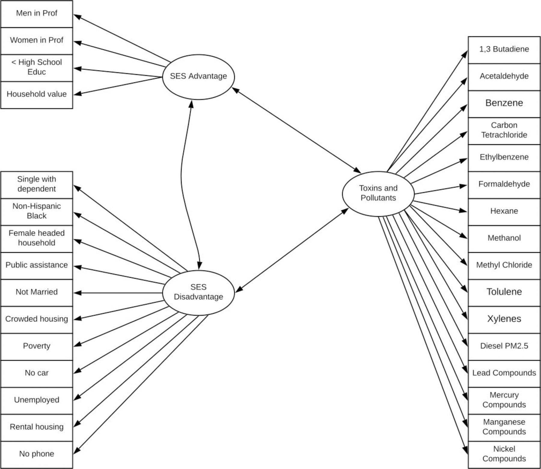
Latent class mixture model for SES and Toxins and Pollutants. The variables in squares denote observed continuous variables and those in circles denote the categorical latent class variables. The arrows describe the relationships between the variables and latent classes.

To pre-process the data, we applied square-root and log-transformations to the SES and pollution data, respectively, to achieve normality for each group of variables since the SES variables are proportions, whereas the pollution data are continuous.

We ran several versions of the model, each with different numbers of classes for each latent variable. For assessing model fit, typical metrics to consider include model convergence, fit statistics such as BIC, AIC and entropy, and class membership, i.e. the percentage of census tracts classified under each level. To assess uncertainty in the best fit model, we examine the probability of a census tract being assigned to a given level, if this probability is high, we can conclude that the assignment has low uncertainty.

We used MPlus (v 1.5 (1)) to run the analysis, which uses maximum likelihood estimation to estimate the level of exposure for each census tract. We also used the R package, MplusAutomation to run the analysis within R, which is a tool that calls MPlus from within R to facilitate pre- and post-processing of data from these models. To evaluate presence of racial disparities in our data, we ran an ANOVA of non-Hispanic black population density versus the low/high SES-Disadvantage, SES-Advantage and pollution latent classes using the R function, lm().

We also conducted K-means clustering on the SES and pollution variables as a comparison. We tested up to 15 clusters using the kmeans() function in R. We evaluated each model using NbClust(), which utilizes several metrics to choose the number of cluster which best fit the data. We computed AIC and BIC in order to compare the fit of the best K-Means model to the LCMM.

Results

We present summary statistics of each SES and pollution variable for a given census tract in North Carolina as compared to the U.S in Table 1. For both SES-Advantage and SES-Disadvantage, the NC averages are higher than the national average. For the pollutant variables, the opposite is true of most VOCs (1,3-Butadiene, Benzene, Ethylbenzene, Hexane, Methyl Chloride and Xylenes), Diesel PM, Lead compounds, Mercury compounds and Nickel compounds. However; Acetalaodehyde, Formaldehyde, and Methanol are higher in NC than the national average.

Table 1.

We compared SES and pollution levels in North Carolina to nationwide levels by examining summary statistics (mean, standard deviation (SD), and interquartile range (IQR)) of the latent and observed variables. For SES data, the mean represents the average proportion of people or households. For the pollution data, the mean represents the average concentration (µg/m³). VOC = volatile organic compounds, PM = particulate matter, HM = heavy metals.

Latent Variable	Observed Variable	U.S.					North Carolina
		Mean	SD	IQR		Mean		SD		IQR
SES Disadvantage	Single parent	0.29	0.16		0.21		0.52		0.14		0.19
	Female head of house	0.21	0.14		0.17		0.45		0.14		0.18
	Crowded household	0.04	0.05		0.04		0.13		0.09		0.12
	Renting	0.35	0.23		0.32		0.56		0.17		0.24
	Phone service	0.97	0.03		0.03		0.99		0.01		0.01
	Below poverty line	0.23	0.31		0.37		0.39		0.39		0.76
	Public assistance	0.03	0.03		0.03		0.12		0.08		0.09
	Unemployed	0.06	0.03		0.04		0.25		0.07		0.08
	No vehicle	0.10	0.13		0.09		0.24		0.12		0.15
	Non-Hispanic Black	0.13	0.22		0.14		0.40		0.23		0.35
SES Advantage	Males - professional	0.07	0.07		0.08		0.20		0.15		0.20
	Females - professional	0.06	0.06		0.07		0.19		0.13		0.17
	< high school education	0.14	0.11		0.13		0.36		0.13		0.19
Pollutants	1,3-Butadiene (VOC)	0.03	0.03		0.03		0.02		0.01		0.02
	Acetaldehyde (VOC)	1.12	0.39		0.48		1.43		0.25		0.25
	Benzene (VOC)	0.42	0.19		0.24		0.37		0.11		0.18
	Carbon Tetrachloride (VOC)	0.53	0.02		0.02		0.53		0.01		0.01
	Ethylbenzene (VOC)	0.14	0.10		0.40		0.10		0.05		0.09
	Formaldehyde (VOC)	1.38	0.42		0.12		1.65		0.26		0.34
	Hexane (VOC)	0.25	0.27		0.65		0.15		0.09		0.09
	Methanol (VOC)	1.36	0.76		0.21		1.47		0.36		0.45
	Methyl Chloride (VOC)	1.15	0.23		0.69		1.14		0.19		0.09
	Toluene (VOC)	1.04	0.80		0.14		0.79		0.37		0.61
	Xylenes (VOC)	0.49	0.37		0.91		0.36		0.20		0.34
	Diesel PM	0.48	0.39		0.47		0.31		0.16		0.22
	Lead Compounds (HM)	0.0008	0.0015		0.0005		0.00047		0.0005		0.00021
	Manganese Compounds (HM)	0.0013	0.0035		0.0009		0.0016		0.0018		0.0008
	Mercury Compounds (HM)	0.0018	0.0005		0.0002		0.0017		0.00031		0.00018
	Nickel Compounds (HM)	0.0006	0.0018		0.0005		0.00025		0.00014		0.000082

The best fit model for NC comprised of mixtures of two levels of Pollutants, two levels of SES-Advantage and two levels of SES-Disadvantage, for a total of eight levels of exposure (Figure 3). We modeled the SES latent variables with two levels to reflect the findings in the Palumbo study⁴⁰. We ran several models with varying levels within the Pollutants latent variable. We found that including more than two levels resulted in non-convergence in the model, so we limited our final model to include only two levels for the pollutant latent variable.

Figure 3.

Estimated latent class membership for each census tract in North Carolina (2014). Each tract is categorized according to level of socioeconomic disadvantage (Disad.), advantage (Adv.) and multi-pollutant exposures (Poln.). Tracts without available data are denoted as NA.

We estimated the mean of each observed variable under each of the eight levels and conclude that the levels or classes within each latent variable can be characterized as low and high. The latent variable profiles are displayed in Figure 2 as bar plots, where the pollution variables are expressed as percentiles and the SES variables are expressed as percents. In the low pollution level, the majority of the pollutants fall around the 20th − 25th percentile, except for mercury, nickel and methyl chloride (40th − 50th percentile). In the high pollution level, almost every pollutant at least doubles; methyl chloride hardly changes, and mercury and nickel only increase roughly to the 60th percentile.

Figure 2.

Barplots of the estimated average value of the variables in the SES-Disadvantage, SES-Advantage and Pollution categories for each latent class. We express each estimated average value as percentages for the SES variables and percentiles for the pollutants.

In areas with low SES-Advantage, on average, the percentage of males and females in professional occupations is estimated to be low (< 5%) while the percentage of people who did not graduate from high school is estimated to be close to 20%. Conversely, in high SES-Advantage areas, the estimated percentage of people in professional occupations rose to roughly 10% for both males and females, while the percentage of the population without a high school degree dropped to around 5%. Examining the SES-Disadvantage latent variable, the model estimates that the following variables are found in higher percentages in the High Disadvantage class as opposed to the low SES-Disadvantage class: no vehicle, public assistance, unemployed, crowded housing, renting, single householder, female householder, below poverty line. We found that phone service was the only SES Disadvantage variable to barely follow this trend: phone service is close to 100% in both the high disadvantage areas and only slightly higher in low disadvantage areas.

We predicted the level of exposure for each census tract, based on the highest predicted class probability for each tract. Overall, 34.1% of the census tracts have high SES-Disadvantage, 66.3% have low SES-Advantage and 59.2% have high mixtures of air pollutants. Our analysis shows that rural areas are sometimes observed under the highest levels of pollution, in addition to metropolitan areas. Areas of high SES-Advantage are concentrated in urban/suburban and coastal areas, while SES-Disadvantage dominates the eastern half of the state as well as many urban areas. Table 2 displays the number of census tracts in each level, as well as the number of those that are rural. In the Census Tract column, the values down the column all sum to the total number of census tracts in North Carolina (N=2174). In the Rural Census Tracts column, each row is the percentage of census tracts in a given exposure level that are classified as rural. For example, in Exposure Level 1, 162 of the 216 census tracts are rural, i.e. 75%.

Table 2.

The LCMM predicts the level of joint exposure to pollutants, socioeconomic advantage and disadvantage for each census tract in North Carolina. This table shows the number of census tracts predicted to belong to each level of exposure. We also display the number of these tracts that are classified as non-metropolitan or rural. In the Census Tract column, values down the column sum to the total number of census tracts in North Carolina (N=2174) and the percents represent a percent of that total. In the Rural Census Tracts column, each row is the percentage of census tracts in a given exposure level that are classified as rural. We defined rural tracts via the Federal Office of Rural Health Policy⁴⁷.

Level	Description of Exposure	Census Tracts	Rural Census Tracts
1	High Disadvantage, Low Advantage and Low Pollution	216 (9.9%)	162 (75%)
2	High Disadvantage, High Advantage and Low Pollution	0 (0%)	0 (0%)
3	Low Disadvantage, Low Advantage and Low Pollution	547 (25.2%)	321 (58.7%)
4	Low Disadvantage, High Advantage and Low Pollution	124 (5.7%)	51 (41.1%)
5	Low Disadvantage, High Advantage and High Pollution	561 (25.8%)	11 (2.0%)
6	Low Disadvantage, Low Advantage and High Pollution	201 (9.2%)	29 (14.4%)
7	High Disadvantage, High Advantage and High Pollution	47 (2.2%)	1 (2.1%)
8	High Disadvantage, Low Advantage and High Pollution	478 (22.0%)	60 (12.6%)

These patterns are visible in Figure 3, which displays estimated exposure level for each census tract in NC. The rural areas of the eastern half of the state are dominated by Level 1 (high disadvantage, low advantage and low pollution) and comprise 9.9% of the census tracts. We did not observe any census tracts in Level 2 (high disadvantage, high advantage and low pollution) due to the fact that the combination of high disadvantage and high advantage is rare⁴⁰.

Level 3 (low disadvantage, low advantage and low pollution) dominates the rural areas of the western half of the state and comprises 25.2% of the census tracts. The most ideal level, Level 4 (low disadvantage, high advantage and low pollution), comprises only 5.7% of the tracts and can be found exclusively in suburban areas throughout the state as well as on the coast.

Level 5 (low disadvantage, high advantage and high pollution) is the most prevalent class with 25.8% membership and is concentrated in urban areas across NC. Level 6 (low disadvantage, low advantage and high pollution) is in a few urban areas in the central part of the state, as well as suburban mountain and inner coastal areas, comprising 9.2% of the census tracts. The smallest exposure level is Level 7 (high disadvantage, high advantage and high pollution) with only 2.2% membership and is found exclusively in urban centers throughout NC. The most toxic class, Level 8 (high disadvantage, low advantage and high pollution) can be found in 22% of the census tracts and is largely located in the urban areas of central NC as well as scattered in rural mountain, inner coastal and coastal areas. This is one of the few levels to associate high pollution with rural areas.

To assess the uncertainty of these predictions, we examined the probabilities of a census tract being assigned to a given level. In the Supplemental Materials (Figure S9), we present a box plot which shows the distribution of assignment probabilities for seven of the eight latent variable levels. Level 2 is not represented since in our analysis, no census tracts were assigned to Level 2. In the case of all levels except Level 7, the median is above 0.80, leading us to believe that there is low uncertainty in the results of our analysis for these levels. The median for Level 7 is approximately 0.75.

Our results also provided insights into economic disparities based on race/ethnicity. Areas with higher SES Disadvantage had significantly higher black population density (p<0.001). Similarly, black population density was higher in areas with higher pollution (p<0.001).

For the K-means clustering analysis, we found that four clusters best fit the data. In the Supplementary Materials (Figures S7 and S8), we provide visualization of the cluster characteristics and the census tract membership in NC. There was a similar pattern of unfavorable SES and Pollution levels in urban areas, and favorable in suburban areas. However, with only four clusters, the clustering from k-means is less nuanced than those from the LCMM. Based on AIC and BIC (lower values are better), the LCMM was a better fit to the data (BIC/AIC for LCMM = −57345.93/−57874.57, BIC/AIC for K-Means = 29646.9/29019.16).

Model Extension for Cancer Disparities

We have proposed an initial framework to link SES and environmental exposures. In Figure 4, we demonstrate how this model can be extended as a means to delineate cancer outcomes disparities. Our future work involves utilizing this novel framework to determine potential modifiable factors that could be employed to reduce disparities in cancer outcomes. Each oval in Figure 4 represents a domain of interest, measured or determined by a set of variables, similar to that shown in Figure 1. Clinical care and access could be measured at the individual level, such as type of insurance, does patient have a PCP, proximity to care. Individual behavior could include physical activity, smoking, alcohol, and other measures that infer higher (or lower) risk. The Biology and Genetics/Ancestry domain could incorporate high-dimensional data, or a smaller set of markers thought to influence cancer outcomes. For high-dimensional data, a variable selection process would also have to be included. Other extensions, such as spatio-temporal correlation will be critical to deepening our understanding of how exposures over time contribute to the development of disease. We continue to work with this ultimate framework in mind, and will share techniques, software, and methods, as they are extended. For different cohorts and diseases that we study, some domains are critical, while others may not be, so we will not always utilize every domain area. But we consider this framework as a starting point for thinking about how to model cancer outcomes disparities. We recognize that there can be many differential exposures, access, behaviors, which may all contribute to the outcomes disparities we see. For example, in studies of breast cancer, we have utilized a biological domain of the sub-typing biomarkers, and we incorporate an association of race as well as one to SES. It is well known that African American women more frequently have triple negative breast cancer, and this likelihood may vary with SES. This modeling framework and methodology provides the ability to flexibly model such relationships.

Figure 4.

Cancer Disparities Modeling Framework. Ovals represent latent variables, informed by multiple indicators, as in the example shown in Figure 1. Rectangles represent available data, used as outcomes or covariates. The dashed arrows demonstrate that race can inform the latent classes across domains, leading to disparities. Race can also inform the cancer outcome, and the model will estimate the separate effect of race on SES and on other domains from the remaining effect of race on outcomes.

Discussion

To our knowledge, this work provides the first framework for an exposure model based on a broad range of SES measures and environmental toxins. The model can also be extended to incorporate cohorts (or trials) with biological measures, clinical care and access, behavioral measures, and health outcomes. LCMMs have the advantage of providing a flexible approach for fitting and testing theoretical relationships. Further, these structures and relationships can be illustrated via diagrams (e.g. Figures 1 and 4), which, though representative of complex statistical models, can be used to bridge knowledge gaps and further research within multi-disciplinary teams of experts by providing accessible visualizations of potential hypotheses to be tested. Also, LCMMs have the added benefit of allowing for uncertainty quantification, an essential modeling feature when it comes to working with results with the potential to inform cancer treatment. We illustrate this advantage by comparing LCMM to a widely used clustering technique, k-means clustering, which not only under-performed in terms of fitting the data, but also lacked any measures of uncertainty in assigning census tracts to exposure clusters/classes. Additionally, the LCMM modeling approach can incorporate the fact that race and SES (as well as other measures), which are typically highly correlated, can be incorporated with that correlation taken into account. This allows us to interpret the impact of SES, which is informed by race, rather than assuming the effect of race is “removed” when controlling for SES. Further, many potential exposures can be incorporated, the mixture of exposures can be tested, and, when planning interventions, areas that exhibit higher risk populations can be easily identified and prioritized.

Gray et al⁴⁸ used modeled predicted surfaces to examine the relationship between air pollution exposure, race, and measures of SES in NC. They considered only PM2.5 and O3 as the pollutants, and assessed poverty, education, and income as SES area level measures from the 2000 census, as well as consideration of the neighborhood deprivation index⁴¹. Similar to our results, they found that PM2.5 was higher in areas with lower SES, higher deprivation, and higher minority population density. Weaver et al²⁶ examined the joint impact of SES and PM2.5 on cardiovascular outcomes. They utilized a hierarchical clustering approach to identify SES groupings, where clusters 1 and 2 exhibited high proportions of black population, impoverished, non-managerial populations, unemployed, and single-parent households; while cluster 3 was urban, with high proportions of college degree, and low poverty, non-managerial and unemployed. These groupings have some similarities to our Disadvantage and Advantage latent classes. In their model, all of the SES variables are in a single domain with multiple levels, while we consider two domains with multiple levels and utilize the association between these two domains. They also noted higher impact of PM2.5 on cardiovascular outcomes in the lower SES areas. Brochu et al⁴⁹, in a PM10 and PM2.5 model in the Northeastern US also found that annual PM was consistently and significantly higher in census tracts with lower socioeconomic position, based on cost of living adjusted median household income. In a review of North American studies of criterion air pollutants and SES⁵⁰, most studies found a similar relationship of higher air pollutants in areas with lower SES. Some exceptions existed to this general pattern, for example in New York City, in a borough-specific analysis, the Bronx, Staten Island, and areas of Manhattan exhibited an opposite pattern. In Los Angeles, PM2.5 and O3 levels were similar across SES, but other pollutants were higher for lower SES.

Previous research has shown that when a latent class level has too few observations, it is not meaningful to include in the model⁵¹. Often in latent models, the AIC, BIC and entropy continue to improve based on increasing the number of latent variable classes and not necessarily based on better fit. This can be mitigated through cross-validation⁵². In our analysis, each individual latent variable has sufficient membership in both the high and low levels (illustrated in Figure S6 of the supplemental materials). We did see sparse membership once we consider the combination of the high and low levels of SES and pollution. In fact, the probability of assignment to Level 2 is non-zero, but it is small in many areas. So, we are not surprised to see that we do not observe any census tracts assigned to Level 2 in North Carolina. We anticipate that if the analysis were repeated for a larger geographic region, we may see a non-zero, but still a small number of tracts assigned to Level 2. Our earlier work identified a small proportion of zip codes assigned to the combination of High Advantage, High Disadvantage⁴⁰. We think this particular combination represents neighborhoods that are in flux, and longitudinally could represent gentrification or decline.

We recognize that the NATA and area-level SES data used do not represent actual individual exposures. However, it is recognized that associations with health outcomes from such area-level measures can be informative. Widely used for health research including cancer studies^53–58, the NATA and ACS data are largely useful for large-scale time trend and spatial analysis and are limited in their usefulness for analysis on a fine spatial and temporal scale. This may be mitigated using data sets with finer spatial and temporal resolution (e.g. EPA’s Federal Reference Method Air Quality Monitors or the Community Multiscale Air Quality Modeling System (CMAQ)) and/or by interpolating the data to achieve higher resolutions⁵⁹. There is ongoing research to develop causal models of environmental exposure on health outcomes, and in that setting, it may be critical to utilize specific exposure data. Future work is needed to extend such causal models to the MPE and SES framework we propose for cancer disparities.

References

- 1.Scharoun-Lee M, Kaufman JS, Popkin BM & Gordon-Larsen P Obesity, race/ethnicity and life course socioeconomic status across the transition from adolescence to adulthood. J. epidemiology community health 63, 133–9, DOI: 10.1136/jech.2008.075721 (2009). [DOI] [PMC free article] [PubMed] [Google Scholar]
- 2.Stringhini S et al. Association of Lifecourse Socioeconomic Status with Chronic Inflammation and Type 2 Diabetes Risk: The Whitehall II Prospective Cohort Study. PLoS Medicine 10, DOI: 10.1371/journal.pmed.1001479 (2013). [DOI] [PMC free article] [PubMed] [Google Scholar]
- 3.Cramb SM, Mengersen KL & Baade PD Identification of area-level influences on regions of high cancer incidence in Queensland, Australia: a classification tree approach. BMC Cancer 11, 311, DOI: 10.1186/1471-2407-11-311 (2011). [DOI] [PMC free article] [PubMed] [Google Scholar]
- 4.Rebbeck TR Prostate Cancer Disparities by Race and Ethnicity: From Nucleotide to Neighborhood. Cold Spring Harb. perspectives medicine 8, a030387, DOI: 10.1101/cshperspect.a030387 (2018). [DOI] [PMC free article] [PubMed] [Google Scholar]
- 5.Conroy SM et al. Racial/Ethnic Differences in the Impact of Neighborhood Social and Built Environment on Breast Cancer Risk: The Neighborhoods and Breast Cancer Study. DOI: 10.1158/1055-9965.EPI-16-0935. [DOI] [PMC free article] [PubMed] [Google Scholar]
- 6.Palmer JR, Boggs DA, Wise LA, Adams-Campbell LL & Rosenberg L Individual and Neighborhood Socioeconomic Status in Relation to Breast Cancer Incidence in African-American Women. Am. J. Epidemiol 176, 1141–1146, DOI: 10.1093/aje/kws211 (2012). [DOI] [PMC free article] [PubMed] [Google Scholar]
- 7.Remington; S. R. S. T.-D. H. M. N. et al. Socioeconomic Risk Factors for Breast Cancer: Distinguishing Individual- and Community-level Effects. Epidemiology 15, 442–450, DOI: 10.1097/01.ede.0000129512.61698.03 (2004). [DOI] [PubMed] [Google Scholar]
- 8.Webster TF, Hoffman K, Weinberg J, Vieira V & Aschengrau A Community- and individual-level socioeconomic status and breast cancer risk: multilevel modeling on Cape Cod, Massachusetts. Environ. health perspectives 116, 1125–9, DOI: 10.1289/ehp.10818 (2008). [DOI] [PMC free article] [PubMed] [Google Scholar]
- 9.Yost K, Perkins C, Cohen R, Morris C & Wright W Socioeconomic status and breast cancer incidence in California for different race/ethnic groups. Cancer Causes Control. 12, 703–711, DOI: 10.1023/A:1011240019516 (2001). [DOI] [PubMed] [Google Scholar]
- 10.Dominici F et al. Fine particulate air pollution and hospital admission for cardiovascular and respiratory diseases. JAMA : journal Am. Med. Assoc 295, 1127–34, DOI: 10.1001/jama.295.10.1127 (2006). [DOI] [PMC free article] [PubMed] [Google Scholar]
- 11.Rappold AG et al. Peat bog wildfire smoke exposure in rural North Carolina is associated with cardiopulmonary emergency department visits assessed through syndromic surveillance. Environ. Heal. Perspectives 119, 1415–1420, DOI: 10.1289/ehp.1003206 (2011). [DOI] [PMC free article] [PubMed] [Google Scholar]
- 12.Feng J & Yang W Effects of Particulate Air Pollution on Cardiovascular Health: A Population Health Risk Assessment. PLoS ONE 7, e33385, DOI: 10.1371/journal.pone.0033385 (2012). [DOI] [PMC free article] [PubMed] [Google Scholar]
- 13.Mar TF et al. PM source apportionment and health effects. 3. Investigation of inter-method variations in associations between estimated source contributions of PM2.5 and daily mortality in Phoenix, AZ. J. Expo. Sci. & Environ. Epidemiol 16, 311–320, DOI: 10.1038/sj.jea.7500465 (2006). [DOI] [PubMed] [Google Scholar]
- 14.Tong Y et al. Association between multi-pollutant mixtures pollution and daily cardiovascular mortality: An exploration of exposure-response relationship. Atmospheric Environ 186, 136–143, DOI: 10.1016/J.ATMOSENV.2018.05.034 (2018). [DOI] [Google Scholar]
- 15.Dominici F, Samet JM & Zeger SL Combining evidence on air pollution and daily mortality from the 20 largest US cities: a hierarchical modelling strategy. J. Royal Stat. Soc. Ser. A (Statistics Soc 163, 263–302, DOI: 10.1111/1467-985X.00170 (2000). [DOI] [Google Scholar]
- 16.Klemm & Robert RJ & Mason MM Aerosol Research and Inhalation Epidemiological Study (ARIES): Air Quality and Daily Mortality Statistical Modeling-Interim Results. J. Air & Waste Manag. Assoc 50, 1433–1439, DOI: 10.1080/10473289.2000.10464188 (2000). [DOI] [PubMed] [Google Scholar]
- 17.Nyberg F et al. Urban air pollution and lung cancer in Stockholm. Epidemiology 11, 487–495, DOI: 10.1097/00001648-200009000-00002 (2000). [DOI] [PubMed] [Google Scholar]
- 18.Pope CA et al. Lung cancer, cardiopulmonary mortality, and long-term exposure to fine particulate air pollution. J. Am. Med. Assoc 287, 1132–1141, DOI: 10.1001/jama.287.9.1132 (2002). [DOI] [PMC free article] [PubMed] [Google Scholar]
- 19.Raaschou-Nielsen O et al. Air pollution and lung cancer incidence in 17 European cohorts: Prospective analyses from the European Study of Cohorts for Air Pollution Effects (ESCAPE). The Lancet Oncol 14, 813–822, DOI: 10.1016/S1470-2045(13)70279-1 (2013). [DOI] [PubMed] [Google Scholar]
- 20.Carver A & Gallicchio VS Heavy Metals and Cancer. In Cancer Causing Substances, DOI: 10.5772/intechopen.70348 (InTech, 2018). [DOI] [Google Scholar]
- 21.Zhao Q et al. Potential health risks of heavy metals in cultivated topsoil and grain, including correlations with human primary liver, lung and gastric cancer, in Anhui province, Eastern China. Sci. Total. Environ 470–471, 340–347, DOI: 10.1016/j.scitotenv.2013.09.086 (2014). [DOI] [PubMed] [Google Scholar]
- 22.Matés JM, Segura JA, Alonso FJ & Márquez J Roles of dioxins and heavy metals in cancer and neurological diseases using ROS-mediated mechanisms, DOI: 10.1016/j.freeradbiomed.2010.07.028 (2010). [DOI] [PubMed] [Google Scholar]
- 23.Coker E, Liverani S, Su JG & Molitor J Multi-pollutant Modeling Through Examination of Susceptible Subpopulations Using Profile Regression. Curr. Environ. Heal. Reports 5, 59–69, DOI: 10.1007/s40572-018-0177-0 (2018). [DOI] [PubMed] [Google Scholar]
- 24.Chi GC et al. Individual and Neighborhood Socioeconomic Status and the Association between Air Pollution and Cardiovascular Disease. Environ. Heal. Perspectives 124, 1840–1847, DOI: 10.1289/EHP199 (2016). [DOI] [PMC free article] [PubMed] [Google Scholar]
- 25.Vieira VM, Villanueva C, Chang J, Ziogas A & Bristow RE Impact of community disadvantage and air pollution burden on geographic disparities of ovarian cancer survival in California. Environ. Res 156, 388–393 (2017). [DOI] [PMC free article] [PubMed] [Google Scholar]
- 26.Weaver AM et al. Neighborhood Sociodemographic Effects on the Associations Between Long-term PM2.5 Exposure and Cardiovascular Outcomes and Diabetes Mellitus. Environ. Epidemiol 3, e038, DOI: 10.1097/EE9.0000000000000038 (2019). [DOI] [PMC free article] [PubMed] [Google Scholar]
- 27.Johns DO et al. Practical advancement of multipollutant scientific and risk assessment approaches for ambient air pollution. Environ. health perspectives 120, 1238–42, DOI: 10.1289/ehp.1204939 (2012). [DOI] [PMC free article] [PubMed] [Google Scholar]
- 28.Davalos AD, Luben TJ, Herring AH & Sacks JD Current approaches used in epidemiologic studies to examine short-term multipollutant air pollution exposures. Annals Epidemiol 27, 145–153, DOI: 10.1016/j.annepidem.2016.11.016 (2017). [DOI] [PMC free article] [PubMed] [Google Scholar]
- 29.Oakes M, Baxter L & Long TC Evaluating the application of multipollutant exposure metrics in air pollution health studies. Environ. Int 69, 90–99, DOI: 10.1016/j.envint.2014.03.030 (2014). [DOI] [PubMed] [Google Scholar]
- 30.Stafoggia M, Breitner S, Hampel R & Basagaña X Statistical Approaches to Address Multi-Pollutant Mixtures and Multiple Exposures: the State of the Science. Curr. Environ. Heal. Reports 4, 481–490, DOI: 10.1007/s40572-017-0162-z (2017). [DOI] [PubMed] [Google Scholar]
- 31.Billionnet C, Sherrill D & Annesi-Maesano I Estimating the Health Effects of Exposure to Multi-Pollutant Mixture. Annals Epidemiol 22, 126–141, DOI: 10.1016/J.ANNEPIDEM.2011.11.004 (2012). [DOI] [PubMed] [Google Scholar]
- 32.Dominici F, Peng RD, Barr CD & Bell ML Protecting Human Health from Air Pollution: Shifting from a Single-Pollutant to a Multi-pollutant Approach NIH Public Access. Epidemiology 21, 187–194, DOI: 10.1097/EDE.0b013e3181cc86e8 (2010). [DOI] [PMC free article] [PubMed] [Google Scholar]
- 33.Keller JP et al. COVARIATE-ADAPTIVE CLUSTERING OF EXPOSURES FOR AIR POLLUTION EPIDEMIOLOGY COHORTS. Ann Appl Stat 11, 93–113, DOI: 10.1214/16-AOAS992SUPP (2017). [DOI] [PMC free article] [PubMed] [Google Scholar]
- 34.Lenters V et al. Prenatal Phthalate, Perfluoroalkyl Acid, and Organochlorine Exposures and Term Birth Weight in Three Birth Cohorts: Multi-Pollutant Models Based on Elastic Net Regression. Environ. Heal. Perspectives 124, 365–372, DOI: 10.1289/ehp.1408933 (2016). [DOI] [PMC free article] [PubMed] [Google Scholar]
- 35.Zanobetti A, Austin E, Coull BA, Schwartz J & Koutrakis P Health effects of multi-pollutant profiles. DOI: 10.1016/j.envint.2014.05.023 (2014). [DOI] [PMC free article] [PubMed] [Google Scholar]
- 36.Pirani M et al. Analysing the health effects of simultaneous exposure to physical and chemical properties of airborne particles. Environ. Int 79, 56–64, DOI: 10.1016/j.envint.2015.02.010 (2015). [DOI] [PMC free article] [PubMed] [Google Scholar]
- 37.Hagenaars JA & Mccutcheon AL Applied Latent Class Analysis (Cambridge University Press, 2002). [Google Scholar]
- 38.Sánchez BN, Budtz-Jørgensen E, Ryan LM & Hu H Structural Equation Models Structural Equation Models: A Review With Applications to Environmental Epidemiology. DOI: 10.1198/016214505000001005 (2005). [DOI] [Google Scholar]
- 39.Hendryx M & Luo J Latent class analysis of the association between polycyclic aromatic hydrocarbon exposures and body mass index. Environ. Int 121, 227–231, DOI: 10.1016/j.envint.2018.09.016 (2018). [DOI] [PubMed] [Google Scholar]
- 40.Palumbo A, Michael Y & Hyslop T Latent class model characterization of neighborhood socioeconomic status. Cancer causes & control : CCC 27, 445–52, DOI: 10.1007/s10552-015-0711-4 (2016). [DOI] [PMC free article] [PubMed] [Google Scholar]
- 41.Messer LC et al. The development of a standardized neighborhood deprivation index. J. urban health : bulletin New York Acad. Medicine 83, 1041–62, DOI: 10.1007/s11524-006-9094-x (2006). [DOI] [PMC free article] [PubMed] [Google Scholar]
- 42.US EPA, O. Hazardous Air Pollutants.
- 43.US EPA, O. 2014 NATA: Assessment Results.
- 44.Hart JE et al. Long-term Particulate Matter Exposures during Adulthood and Risk of Breast Cancer Incidence in the Nurses’ Health Study II Prospective Cohort. Cancer Epidemiol. Biomarkers & Prev 25, 1274–1276, DOI: 10.1158/1055-9965.EPI-16-0246 (2016). [DOI] [PMC free article] [PubMed] [Google Scholar]
- 45.Bureau UC American Community Survey 1-Year Data (2011–2017).
- 46.Blake KS, Kellerson RL & Simic A Measuring Overcrowding in Housing. Tech. Rep (2007).
- 47. Federal Office of Rural Health Policy (FORHP) Data Files | Official web site of the U.S. Health Resources & Services Administration.
- 48.Gray SC, Edwards SE & Miranda ML Race, socioeconomic status, and air pollution exposure in North Carolina. Environ. Res 126, 152–158, DOI: 10.1016/J.ENVRES.2013.06.005 (2013). [DOI] [PubMed] [Google Scholar]
- 49.Brochu PJ et al. Particulate air pollution and socioeconomic position in rural and urban areas of the Northeastern United States. Am. J. Public Heal 101, 224–30, DOI: 10.2105/AJPH.2011.300232 (2011). [DOI] [PMC free article] [PubMed] [Google Scholar]
- 50.Hajat A, Hsia C & O’Neill MS Socioeconomic Disparities and Air Pollution Exposure: a Global Review. Curr. Environ. Heal. Reports 2, 440–450, DOI: 10.1007/s40572-015-0069-5 (2015). [DOI] [PMC free article] [PubMed] [Google Scholar]
- 51.Eppig JS et al. Statistically Derived Subtypes and Associations with Cerebrospinal Fluid and Genetic Biomarkers in Mild Cognitive Impairment: A Latent Profile Analysis. J. Int. Neuropsychol. Soc. : JINS 23, 564–576, DOI: 10.1017/S135561771700039X (2017). [DOI] [PMC free article] [PubMed] [Google Scholar]
- 52.Grimm KJ, Mazza GL & Davoudzadeh P Model Selection in Finite Mixture Models: A k -Fold Cross-Validation Approach. Struct. Equ. Model. A Multidiscip. J 24, 246–256, DOI: 10.1080/10705511.2016.1250638 (2017). [DOI] [Google Scholar]
- 53.Krieger N Geocoding and Monitoring of US Socioeconomic Inequalities in Mortality and Cancer Incidence: Does the Choice of Area-based Measure and Geographic Level Matter?: The Public Health Disparities Geocoding Project. Am. J. Epidemiol 156, 471–482, DOI: 10.1093/aje/kwf068 (2002). [DOI] [PubMed] [Google Scholar]
- 54.Krieger N Overcoming the absence of socioeconomic data in medical records: Validation and application of a census-based methodology In American Journal of Public Health, vol. 82, 703–710, DOI: 10.2105/AJPH.82.5.703 (American Public Health Association, 1992). [DOI] [PMC free article] [PubMed] [Google Scholar]
- 55.Apelberg BJ, Buckley TJ & White RH Socioeconomic and racial disparities in cancer risk from air toxics in Maryland. Environ. Heal. Perspectives 113, 693–699, DOI: 10.1289/ehp.7609 (2005). [DOI] [PMC free article] [PubMed] [Google Scholar]
- 56.George BJ et al. An evaluation of EPA’s National-Scale Air Toxics Assessment (NATA): Comparison with benzene measurements in Detroit, Michigan. Atmospheric Environ 45, 3301–3308, DOI: 10.1016/j.atmosenv.2011.03.031 (2011). [DOI] [Google Scholar]
- 57.Zhou Y, Li C, Huijbregts MA & Mumtaz MM Carcinogenic air toxics exposure and their cancer-related health impacts in the United States. PLoS ONE 10, DOI: 10.1371/journal.pone.0140013 (2015). [DOI] [PMC free article] [PubMed] [Google Scholar]
- 58.McEntee JC & Ogneva-Himmelberger Y Diesel particulate matter, lung cancer, and asthma incidences along major traffic corridors in MA, USA: A GIS analysis. Heal. Place 14, 817–828, DOI: 10.1016/j.healthplace.2008.01.002 (2008). [DOI] [PubMed] [Google Scholar]
- 59.Lawson AB, Choi J, Cai B, Hossain M, Kirby RS and Liu J, 2012. Bayesian 2-stage space-time mixture modeling with spatial misalignment of the exposure in small area health data. Journal of agricultural, biological, and environmental statistics, 17(3), pp.417–441. [DOI] [PMC free article] [PubMed] [Google Scholar]
Associated Data
This section collects any data citations, data availability statements, or supplementary materials included in this article.