Abstract
We test for the existence of volatility spillovers and co-movements among energy-focused corporations during the outbreak of the COVID-19 pandemic, inclusive of the April 2020 events where West Texas Intermediate (WTI) oil future prices became negative. Employing the spillover index approach of Diebold and Yilmaz (2012); as well as developing a DCC-FIGARCH conditional correlation framework and using estimated spillover indices built on a generalised vector autoregressive framework in which forecast-error variance decompositions are invariant to the variable ordering, we examine the sectoral transmission mechanisms of volatility shocks and contagion throughout the energy sector. Among several results, we find positive and economically meaningful spillovers from falling oil prices to both renewable energy and coal markets. However, this result is only found for the narrow portion of our sample surrounding the negative WTI event. We interpret our results being directly attributed to a sharp drop in global oil, gas and coal demand, rather than because of a sudden increase in oil supply. While investors observed the US fracking industry losing market share to coal, they also viewed renewables as more reliable mechanism to generate long-term, stable and low-cost supply.
Keywords: Oil prices, Oil and gas corporations, Volatility spillovers, Volatility co-movement, Market linkage, Financial crisis, Contagion
Highlights
-
•
Firm-level analysis during negative WTI oil
-
•
Test for volatility spillovers and co-movements among energy-focused firms
-
•
Spillovers and co-movements during COVID-19 and negative WTI oil
-
•
Spillovers from falling oil prices to renewable energy and coal
1. Introduction and motivations
We examine volatility spillovers and co-movements among energy-focused corporations during the COVID-19 pandemic. Our particular focus is on the extraordinary event in April 2020 where West Texas Intermediate (WTI) oil future prices became negative. Developing a DCC-FIGARCH conditional correlation framework and using estimated spillover indices built on a generalised vector autoregressive framework in which forecast-error variance decompositions are invariant to the variable ordering, we examine the sectoral transmission mechanisms of volatility shocks and contagion throughout the energy sector.
1.1. Context
This investigation has considerable contextual background. We are focused on directional spillovers, and co-movements of energy-related companies during both the COVID-19 pandemic and during a time when WTI oil fell dramatically to negative prices. The context of COVID-19, and the concomitant economic, social, and market turmoil is of course relevant in a broad set of potential ways. For instance, Goodell (2020) notes a number of possible long-term adjustments to financial systems stemming from COVID-19, including possibly less use of leverage by firms and households and a greater pricing of equity risk. But the period of our study overlaps the extraordinary fall of WTI prices, which though related to the economic fallout from COVID-19, had its own mechanisms.
However, there are other contextual aspects that need to be described. As the unprecedented fall in WTI oil prices in April 2020 occurred during the economic turmoil ensuing from the COVID-19 pandemic, during this time oil traders were contending with broadly attempting to quantify the severity of the COVID-19 and its influence on worldwide demand for oil; as well as assessing broad oil-related geopolitical issues related to the relationship between Saudi Arabia and Russia. In early March 2020, Saudi Arabia sharply cut the price of the oil it supplied to Asia, Europe, and the US, which led to a subsequent collapse in worldwide oil prices, stock markets, and the Russia Rouble. In the following days, Saudi Arabia then proceeded to announce an increase in production. This was widely seen as an attempt by Saudi Arabia to increase world supply by approximately 25%, for competitive reasons. However, this action by Saudi Arabia was met by a challenging response from Russia in which they increased their production and supply in a similar manner. Considering the sharp fall in demand sourced within the continuous escalation of the COVID-19 pandemic, this increased supply caused a fall in oil prices to a 17-year low of almost $20 per barrel. After broad international political intervention in April 2020, a cut in production was agreed. However, even considering this agreement, world stockpiles were estimated by the International Energy Agency to have increased by approximately 15 million barrels per day. Such broad geopolitical tensions, concomitant with COVID-19, rapidly produced sector-disrupting reverberations. What followed was the incredible situation where the WTI delivery price difference between months resulted in unusually high contango, and subsequent negative pricing due to depressed demand and insufficient storage capacity.1
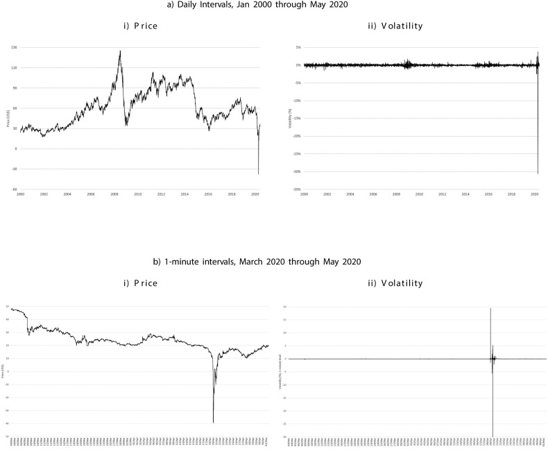
Fig. 1 illustrates both the short-term and long-term WTI prices and volatility against time over the important period of gradually increasing global acknowledgement of the COVID-19 threat. Trading in a range between $50–$60 during October through December 2019, the price of WTI did not initially present evidence of substantial variability. Looking at the long-term price trend, we clearly observe the scale of the recent price collapse, which extended close to $184 below the price of WTI that occurred during the subprime crisis of 2008. Starting from a price of around $60 when the COVID-19 pandemic was first identified by the World Health Organisation (WHO) in late-December 2019, it was not until early-March 2020 before WTI fell below $30. In mid-April, it sharply fell below $20 before proceeding to rapidly fall below zero. Between 17 April and 20 April, the price of WTI fell from $18 to –$37.
Fig. 1.
West Texas intermediate high-frequency price and volatility, 1-min data.
Note: The above data represents hourly WTI price and volume behaviour for the period March 2019 through May 2020. Data was obtained from Thomson Reuters Eikon.
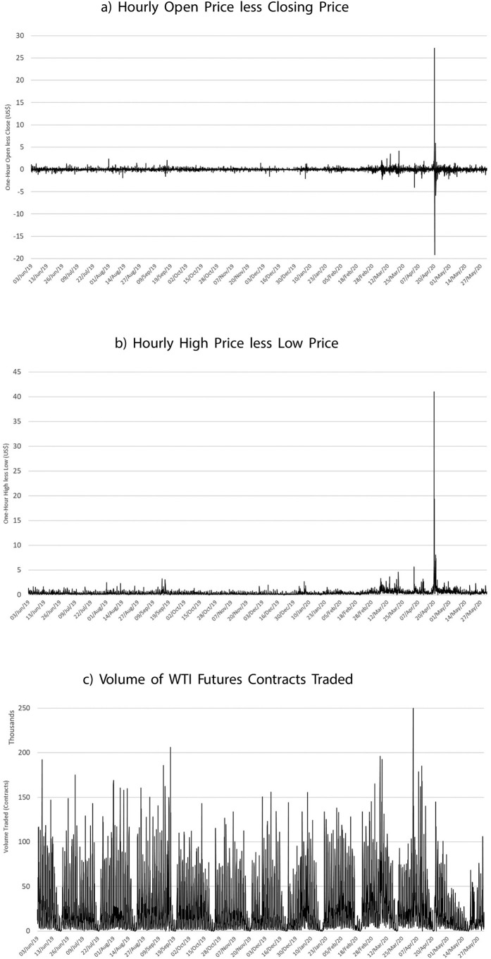
In Fig. 2 we observe the hourly nominal price change along with the difference between hourly high and low prices. Examining Fig. 2, the magnitude of the hourly changes in WTI prices is evident. While the largest hourly trading volume of WTI futures contracts occurs on 20 April, pronounced elevated levels of liquidity are evident throughout 2020.
Fig. 2.
West Texas intermediate high-frequency price and volume behaviour (1-h data).
Note: The above data represents hourly WTI price and volume behaviour for the period March 2019 through May 2020. Data was obtained from Thomson Reuters Eikon.
We must remember that negative oil prices suggest oil producers are paying buyers to take their production, largely due to fears that storage capacity could run out in the short-term. Negative oil prices reflect a situation where oil firms must resort to renting tankers to store surplus supply. This negative pricing is driven in part by a technicality of the global oil market: oil is traded on its future price and traders do not want to take delivery of the oil and incur storage costs. While international oil prices did not decline as much as WTI, depressed WTI prices also affected firms operating in the North Sea and Middle East. Similar duration contracts for Brent crude, the benchmark for global oil prices, were down approximately 25% during the same time period as WTI prices went negative. The reason for the difference between the Brent and WTI benchmarks can be explained by differential storage costs. Brent crude is priced in the middle of the North Sea, where tanker storage is ample and accessible, while WTI oil storage in the US is limited. WTI is also landlocked, while North Sea isolation allows Brent more shielding and flexibility to respond to shifting coronavirus demand shocks.
Our research analyses and examines volatility spillovers and volatility co-movements among energy-producing, extracting, and transporting corporations' stock prices over the period May 2019 through May 2020, incorporating both the period inclusive of the outbreak of the COVID-19 pandemic, and the exceptionally rare period when WTI oil prices turned negative.
1.2. Background literature
During the period of our study, we investigate co-movements and spillovers across significant firms in eight energy-related Thomson Reuters Business Classifications. The spillover index approach of Diebold and Yilmaz (2009); as well as the DCC-FIGARCH procedure (an extension of the work of Engle, 2002) are used to identify the transmission mechanism of volatility shocks and the contagion of volatility. Therefore, it is relevant to review important and recent literature regarding the interaction of oil and stock prices.
A number of studies focus on the effects and influence of WTI and other similar oil markets on a variety of international stock markets, while developing on a number of differing volatility methodologies. For instance, Du and He (2015) find that, prior to the 2008 financial crisis, there were positive risk spillovers from stock market to crude oil market, and negative spillovers from crude oil market to stock market. However, they also find, post 2008, a strengthening of bidirectional positive risk spillovers with asymmetric correlations. Analysing data back to 1859, Balcilar et al. (2017) finds that both oil and S&P 500 prices share a common stochastic trend. Other studies have examined the impact of oil on the stock market of China (Kang et al., 2010; Yang et al., 2015); Japan and Korea (Kang et al., 2009); the US (Ho et al., 2013); and broad G7 indices (Beine et al., 2008; Bentes, 2014). Zhang (2017) analyses the relationship between oil shocks and returns at six major stock markets around the world to find evidence that the contribution of oil shocks to the world financial system is quite limited, while Maghyereh et al. (2016) finds evidence of connectedness between oil and equity is established by the bi-directional information spillovers between the markets. Arouri et al. (2012) and Antonakakis et al. (2018) also examine the interaction of oil prices and stock markets. Chaining together oil, economic policy uncertainty and equity prices, Antonakakis et al. (2014) find that economic policy uncertainty responds negatively to aggregate demand oil price shocks, while GMM examine EPU on US equities (see also Xu et al., 2019; Yang, 2019).
Similar methodologies have been used to investigate for the presence of volatility spillovers in stock markets (Awartani and Maghyereh, 2013; Bekiros et al., 2018; Liow, 2015; Shahzad et al., 2017).2 Alternatively, Salisu and Oloko (2015) identify results somewhat contrasting to other literature, identifying a significant positive return spillovers from the US stock market to oil markets.
While there has been much examination of the interaction between oil prices and stock markets and a small number of papers analysing the effects of oil volatility on the returns of oil and gas corporations, there has been little or no investigations of these topic with regard to the conditioning role of pandemics, or negative oil price effects.3
1.3. Oil and renewables
In this paper, our primary focus is on co-movement and spillovers from oil to renewables under extreme oil price movements. And so it is particularly relevant to consider recent work that examine the interactions between oil and renewable energy. A large number of recent papers find that renewables and oil co-move in the same direction. These papers include Apergis and Payne (2014); Ferrer et al. (2018); Khan et al. (2017); Reboredo (2015); Reboredo et al. (2017); Sadorsky (2009); Sadorsky (2012a) and Sadorsky (2012b).4 Some of these papers suggest reasons for a positive co-movement between oil and renewables, while others simply observe findings. It is reasonable to suppose that all forms of energy might move together with levels of energy demand. Maghyereh et al. (2019) suggest that stability of oil is important for renewables.
On the other hand, the enormous economic impact of COVID-19 and the concomitant shock to the oil industry of negative WTI prices, presents a need for a revisiting of the interaction of oil and renewables, especially during extreme conditions. While not yet covered in academic literature, a number of recent trade articles have suggested COVID-19 specifically will be a boom for renewals. The reasoning of these trade articles is generally that COVID-19 will in many regions revise downward expectations of future energy needs. Consequently, renewables will be more seen as a reasonable alternative to meet energy needs.
In this paper we exploit the unprecedented global economic downturn conditions of COVID-19 to test two alternative hypotheses regarding the co-movement of oil and renewables. We consider a price-competition hypothesis in which, as oil prices sharply fall, there will be a replacement of renewables with less expensive oil.
H1
An extreme fall in oil prices will lead to a fall in the price of renewables.
Alternatively we consider a global demand hypothesis in which a severe fall in oil prices stemming from a sharp decline in global demand for energy will engender energy planners to regard renewables as a more reliable long-term first-choice for energy needs, as it will be more likely for renewables to meet energy needs.
H1a
: An extreme fall in oil prices will lead to a rise in the price of renewables.
In considering our hypotheses, we note that Kumar et al. (2012) frame the issue of how renewables will react to changes in oil prices. Kumar et al. (2012) suggest on the one hand that an increase in oil prices will impact stocks, including renewables, negatively. This is because of the direct and indirect role of oil prices in production costs. A negative and significant relationship between oil prices and equities has been demonstrated by previous research (e.g., Cong et al., 2008; Henriques and Sadorsky, 2008; Huang et al., 1996; Jones and Kaul, 1996; Miller and Ratti, 2009; Park and Ratti, 2008; Sadorsky, 2009). In this vein, we might expect a fall in oil prices to favourably impact stocks, including renewables. However, with particular regard to renewables, this has been found not to be strongly the case (Henriques and Sadorsky, 2008). Further, this was clearly not the case for equity markets in general for the period of our study, with the downturn in global demand and disruptions in supply chains during this time additional factors.
Kumar et al. (2012) also suggest, alternatively, a substitution theory which posits renewables will gain when oil prices are higher as the cost of renewables is concomitantly more affordable. However, as oil prices fell, we observe a gain for renewables. Considering the context of our investigation, what previous important theory does not consider, understandably, is the conditioning role of a shock to global demand and supply chains of the impact of COVID-19. Consequently, our study is difficult to frame in comparison to previous investigations. Overall, there are a number of contextual factors for our study that have been insufficiently investigated. First, is there is a previously unidentified relationship between specifically oil storage costs and the economic attractiveness of renewables? Second, does an enormous downward shock to global demand prospects lead to equity and venture capital investments in renewables being more attractive? The notion here is that there will be greater confidence that renewables will be enough to meet needs. This is the argument put forth in recent trade articles. However, we are not aware of previous academic literature addressing this rather vital issue. Third, as global supply chains are disrupted, in this case to an extent without recent precedent, and countries overall stepped back from participation in the global economy, were renewables seen as more favourable local sourcing of energy? Fourth, an argument we particularly highlight in the paper, renewables may have gained in the context of negative WTI prices particularly on the collapse of optimism in the fracking industry. We draw indirect inferences from results for the coal industry gaining, in addition to renewables, as WTI oil fell. We consider this explanation as well in the context of the current geopolitical issues related to the fracking industry. Coal can also be seen, particularly for the US as having a similar supply-chain advantage to renewables. These four reasons, not exclusive to each other, are all plausible explanations for our results. We acknowledge our results raise important questions and might challenge existing theoretical underpinnings. Additionally, our results may be highly context-driven. But the context of negative oil prices during a pandemic is too important for research to ignore.
Overall, our results, when collectively examined, suggest the extraordinary fall in WTI to negative prices was seen by energy investors as due to a sharp drop in global demand rather than due to a sharp increase in oil supply by Saudi Arabia as part of a situational challenge to the USA fracking industry.
In this paper, we employ the spillover index approach of Diebold and Yilmaz (2009); as well as the DCC-FIGARCH procedure (an extension of the work of Engle, 2002) to identify the transmission mechanism of volatility shocks and the contagion of volatility across firms in eight Thomson Reuters Business Classifications. Our analysis incorporates both high-frequency and daily time series data of stock prices of the largest oil and gas companies for the period October 2019 through May 2020. Our period of study allows us to compare and contrast volatility and volatility spillovers among four different sub-periods: i) pre-pandemic; ii) during the Chinese denoted outbreak of ‘mystery pneumonia’; iii) the official World Health Organisation (WHO) announcement of COVID-19; and iv) the effects of negative oil prices during the period both inclusive of 20 April 2020 and the period thereafter.
Most importantly, we find positive and economically meaningful spillovers from falling oil to renewables. However this result is only found for the narrow portion of our period of study around the negative WTI event. This finding differs from most previous research that finds that renewables and oil positively co-move, and differs from what we find in other sub periods of our sample. However, previous research has not been able to assess the co-movements of oil and renewables under such an extreme economic downturn as during the COVID-19 pandemic. Although not the primary focus of our study, we also find a negative co-movement of oil and coal. While oil fell to unprecedented lows, there was a directional spillover that elevated coal industries. We exploit this finding of a co-movement of oil and coal to conclude that our result of renewables gaining as oil fell was due to investors seeing the extraordinary fall in WTI as stemming from a sharp drop in global demand, rather than because of a sudden increase in oil supply. If, alternatively, the latter explanation was true we would have seen coal also fall for competitive price reasons. In a state of starkly declining global growth prospects, investors saw the US fracking industry losing to coal, they also viewed renewables as more reliable to generate long-term supply.
The remained of the paper is structured as follows: in Section 2 we describe the data and in Section 3 the methodology used to analyse; empirical results are provided in Section 4, while both discussion and concluding comments are provided in Section 5.
2. Data
The sample period for data collection is chosen from 1 May 2019 through 12 May 2020, inclusive of one-year of hourly price observations,5 a total of 6293 hourly observations. We develop on high-frequency trading data obtained from Thomson Reuters Eikon for both West Texas Intermediate Oil (WTI) and the sixty-nine energy stocks with associated summary statistics presented in Table 1 and an outline of each stock presented in Table A1 of the attached appendices. As with Antonakakis et al. (2018), we define the stock (i) price volatility as the absolute return6 V it = ∣ lnP it − lnP it−1∣, where P it is the hourly closing price of the stock on day t. The price of WTI throughout this analysis is represented as variable j. Eight sectors are defined based on their related TRBC Sector Code. We analyse the effects of WTI price behaviour on that of: a) Oil & Gas Exploration & Production; b) Oil & Gas Refining & Marketing; c) Integrated Oil & Gas; d) Oil-related Services & Equipment; e) Oil & Gas Transportation Services; f) Oil & Gas Drilling; g) Coal; and h) Renewable Energy. As noted by Antonakakis et al. (2018), while the use of firm level data to analyse relationships between sectors is relatively new (e.g., Aggarwal et al., 2012; Boyer and Filion, 2007; Phan et al., 2016), investigations at the firm level of interactions of both returns and volatilities (e.g., Antonakakis et al., 2018) are much less common.
Table 1.
Summary statistics based on sectoral price volatility (by denoted period).
| O&G explor. | O&G refin. | Integ. O&G | O&G S&Eq. | O&G trans. | O&G drill. | Coal | R.Energy | |
|---|---|---|---|---|---|---|---|---|
| Before COVID-19 | ||||||||
| Mean | −0.0002 | 0.0001 | −0.0002 | −0.0002 | 0.0000 | −0.0004 | −0.0004 | 0.0001 |
| Variance | 0.0000 | 0.0000 | 0.0001 | 0.0000 | 0.0000 | 0.0002 | 0.0000 | 0.0000 |
| Skewness | −0.4643 | −0.5429 | −0.1366 | −0.6277 | −0.1018 | 0.3888 | −1.0055 | −0.7548 |
| Kurtosis | 6.0903 | 7.4979 | 12.4128 | 7.0368 | 10.9248 | 15.6173 | 15.6995 | 12.8746 |
| Minimum | −0.0406 | −0.0282 | −0.0891 | −0.0379 | −0.0257 | −0.0996 | −0.0609 | −0.0509 |
| Maximum | 0.0268 | 0.0167 | 0.0623 | 0.0315 | 0.0340 | 0.1247 | 0.0347 | 0.0474 |
| Chinese-confirmed pneumonia | ||||||||
| Mean | 0.0003 | −0.0001 | 0.0004 | 0.0005 | 0.0004 | 0.0005 | −0.0004 | 0.0005 |
| Variance | 0.0000 | 0.0000 | 0.0000 | 0.0000 | 0.0000 | 0.0001 | 0.0002 | 0.0000 |
| Skewness | 0.8712 | 0.1362 | 0.4342 | 0.4358 | 0.4823 | 0.9230 | −11.0622 | −0.1196 |
| Kurtosis | 6.7401 | 6.7153 | 6.2633 | 8.1000 | 3.5857 | 5.6805 | 177.1660 | 3.6085 |
| Minimum | −0.0227 | −0.0143 | −0.0274 | −0.0260 | −0.0124 | −0.0340 | −0.2015 | −0.0218 |
| Maximum | 0.0238 | 0.0139 | 0.0355 | 0.0258 | 0.0141 | 0.0619 | 0.0364 | 0.0207 |
| WHO-confirmed COVID-19 | ||||||||
| Mean | −0.0004 | −0.0004 | −0.0016 | −0.0008 | −0.0004 | −0.0001 | −0.0005 | 0.0002 |
| Variance | 0.0002 | 0.0002 | 0.0008 | 0.0002 | 0.0002 | 0.0010 | 0.0004 | 0.0002 |
| Skewness | 0.4975 | 0.8250 | 2.5959 | −0.7128 | −0.0421 | 2.3340 | 1.1882 | −0.2600 |
| Kurtosis | 11.8352 | 14.4664 | 30.5347 | 7.3994 | 12.5880 | 23.9301 | 12.4862 | 10.0720 |
| Minimum | −0.0887 | −0.0578 | −0.1354 | −0.0728 | −0.1031 | −0.1560 | −0.0887 | −0.1004 |
| Maximum | 0.1152 | 0.1148 | 0.3107 | 0.0722 | 0.0949 | 0.3432 | 0.1598 | 0.1023 |
| Negative WTI prices and after | ||||||||
| Mean | 0.0015 | 0.0010 | 0.0017 | 0.0012 | 0.0010 | 0.0038 | 0.0006 | 0.0007 |
| Variance | 0.0003 | 0.0002 | 0.0012 | 0.0003 | 0.0002 | 0.0016 | 0.0005 | 0.0002 |
| Skewness | 0.1352 | 0.6487 | 0.9085 | −0.5200 | −0.2916 | 2.9514 | 0.1474 | 0.0168 |
| Kurtosis | 3.8145 | 9.4841 | 5.7264 | 3.5844 | 3.2466 | 19.7679 | 4.1260 | 3.6318 |
| Minimum | −0.0651 | −0.0578 | −0.1262 | −0.0717 | −0.0597 | −0.1238 | −0.0887 | −0.0755 |
| Maximum | 0.0924 | 0.1148 | 0.1973 | 0.0722 | 0.0514 | 0.3432 | 0.1135 | 0.0665 |
Note: The above data represents hourly sectoral price volatility for the period March 2019 through May 2020. Data was obtained from Thomson Reuters Eikon.
Due to issues with market liquidity, only companies with market capitalisation above $50 million as of January 2020 are included in this analysis. The scale and direction of both volatility spillovers and directional volatility spillovers will provide substantial information with regards to broad energy market dynamics during immense periods of economic turmoil, but also potential channels through which diversification opportunities exist. There is also particular interest of the latter included sectors representing both coal and renewable energy, and as to whether their price behaviour and interaction varies with that of traditional Oil & Gas-related companies.
In Table 2 , we observe the hourly price-related summary statistics of WTI during the four denoted periods of analysis, relating to the pre-COVID-19 periods and those relating to the China-specific outbreak of COVID-19, the contagion of COVID-19 throughout the world as identified by the official WHO announcement, and finally, when the price of WTI turned negative, inclusive of the period thereafter. Such results offer substantial information with regards to hourly nominal price volatility and recorded trading volumes as representative of market liquidity. It becomes quickly apparent that there is little differentials between that of the period prior to COVID-19 and the period denoted to surround the announcement of a ‘mystery pneumonia’ in China. Such a results supports the findings of (Conlon et al. (2020) and Corbet et al., 2020a, Corbet et al., 2020b), that there exist little evidence of worldwide contagion or information flows due to available Chinese news. While Chinese-traded oil did show contagion effects through apparent flight-to-safety behaviour, there is little to suggest that WTI exhibits similar characteristics. However, the period after the official identification of the COVID-19 outbreak by the WHO is very different. Hourly volatility levels increase sharply during this period, with differentials in hourly high and low pricing presenting evidence of two and three times the scale of prior averages. Trading volumes differ substantially, with average hourly levels initially increasing after the WHO announcement, however, they fall by almost 50% in the period after the negative price event in WTI. There are sharp increases in both the skew and kurtosis of these price and liquidity dynamics during the COVID-19 outbreak, which is further exhibited in the incredibly large one-hour changes in prices during this time. Specifically, in the period after 20 April, there exists a single hour when the differential between high and low pricing was $41.02 and the difference between open and closing price was $27.19.
Table 2.
West Texas intermediate price and volume summary statistics (1-h frequency).
| Open - close | High - low | Trade volume | |
|---|---|---|---|
| Before COVID-19 | |||
| Mean | 0.0026 | 0.3246 | 24,005 |
| Variance | 0.0585 | 0.0635 | 8.813E+08 |
| Skewness | 0.6720 | 2.9730 | 1.9951 |
| Kurtosis | 10.1406 | 18.7728 | 4.3390 |
| Minimum | −1.8500 | 0.0000 | 1.0000 |
| Maximum | 2.3200 | 3.2400 | 205,945 |
| Observations | 2741 | 2741 | 2741 |
| Chinese-confirmed pneumonia | |||
| Mean | −0.0044 | 0.2206 | 16,884 |
| Variance | 0.0295 | 0.0375 | 6.027E+08 |
| Skewness | −0.2584 | 3.0262 | 2.4793 |
| Kurtosis | 20.1092 | 16.7649 | 6.9683 |
| Minimum | −1.5800 | 0.0000 | 2.0000 |
| Maximum | 1.4400 | 1.9900 | 155,770 |
| Observations | 680 | 680 | 680 |
| WHO-confirmed COVID-19 | |||
| Mean | 0.0197 | 0.4813 | 27,813 |
| Variance | 0.1454 | 0.1828 | 9.716E+08 |
| Skewness | 0.5768 | 3.6543 | 1.9283 |
| Kurtosis | 22.1409 | 24.6966 | 4.7993 |
| Minimum | −3.9900 | 0.0000 | 1.0000 |
| Maximum | 4.1000 | 5.6400 | 252,564 |
| Observations | 1759 | 1759 | 1759 |
| Negative oil and the period thereafter | |||
| Mean | −0.0282 | 0.8009 | 15,209 |
| Variance | 2.1322 | 3.7028 | 3.786E+08 |
| Skewness | 5.8884 | 15.1472 | 2.5739 |
| Kurtosis | 217.7028 | 288.9440 | 8.6227 |
| Minimum | −19.1600 | 0.0000 | 1.0000 |
| Maxumum | 27.1900 | 41.0200 | 144,700 |
| Observations | 697 | 697 | 697 |
Note: The above data represents hourly WTI price and volume behaviour for the period March 2019 through May 2020. Data was obtained from Thomson Reuters Eikon.
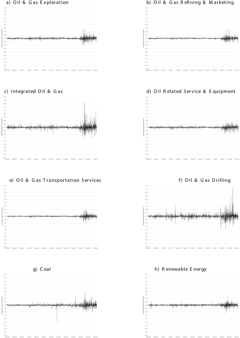
In Fig. 3 , we observe for the same time period the hourly price volatility of each of the included sectors analysed in comparison to price movements within the market for WTI. It is noticeable that there exist a wide-variety of response to the selected windows of investigation surrounding COVID-19. Associated summary statistics are presented in Table 1. Sectors representing both Oil & Gas Drilling and Integrated Oil & Gas are found to be the most volatile throughout all of the analysed periods, and particularly so in the period after the outbreak of COVID-19. While coal markets, which could be argued to be relatively isolated to shocks within WTI present evidence of simultaneously elevated volatility, estimates within companies denoted to be working in the renewable energy sector appear to to behave in quite a moderated manner, similar to companies working in the sectors for oil & gas servicing, equipment development and broad transportation.
Fig. 3.
Energy sector price volatility, 1-h data (1 January 2019 through 1 May 2020).
Note: The above data represents hourly sectoral price volatility for the period March 2019 through May 2020. Data was obtained from Thomson Reuters Eikon.
To analyse the differential behaviour and influence of WTI upon energy stocks in the US through this period of immense economic disruption, we separate our analysis into a number of pre-determined and robust sub-periods. The first sub-period runs from 1 May 2019 through 16 November 2019. This selection is made due to the media identification on the 17 November 2019 of the first case of COVID-19 detected in mainland China, as reported by the South China Morning Post (as per (Conlon et al. (2020), Corbet et al. (2020b) and Corbet et al. (2020a)). Hence, the sub-period is the first stage without the latent impacts of COVID-19. The second sub-period is from 17 November 2019 through 30 December 2019. On the 30 December 2019, as reported by World Health Organisation (WHO), Wuhan Municipal Health Commission in China reported a cluster of cases of pneumonia in Wuhan, Hubei Province. The novel coronavirus, in its current form was subsequently identified and announced to the world as a global pandemic. After this date, the COVID-19 was gradually acknowledged by the globe and its impacts became internationally contagious. And a third sub-period which is from 31 December 2019 through 19 April 2020, defining a stage where the COVID-19 pandemic subsequently spreads out of China and begins a widespread contagious period to the rest of the world. The final sub-period is of particular interest, as it is inclusive of the sharp negative fall of WTI prices and that of 20 April when the price of the forthcoming May expiring futures contracts sold on exchange at a price of -$37.63. Such negative prices had not been observed in the largest oil markets at any point in recorded history, presenting evidence of the broad rarity of such an event, to which the confusion and panic observed on 20 April 2020 manifested.
3. Empirical methodology
3.1. DCC-FIGARCH volatility estimates
In the first stage of our analysis, we focus on the estimation of the traditional dynamic conditional correlations of the energy sector with that of WTI. To do so, we build on the dynamic conditional correlation methodology (DCC-GARCH) of Engle (2002), who decomposed the conditional covariance matrix as:
| (1) |
| (2) |
| (3) |
where R t is defined as the conditional correlation matrix and D t is a diagonal matrix with time-varying standard deviations on the main diagonal. Further, Q t is identified as the approximation of the conditional correlation matrix, defined above in Eqs. (1), (2) as R t, where the positive semi-definiteness of Q t is guaranteed if both α and β are both positive, while the sum of both α and β is less than one while the initial matrix (Q 1) being positive. , where representing the unconditional average correlation. We next estimate D t, which is defined as the conditional volatility through the use of a univariate long-memory methodology, where we divide the returns by their conditional volatility and use the ε t = D t −1 r t to estimate the quasi-conditional correlation matrix Q t. Q t is re-scaled to obtain the conditional correlation matrix described in Eq. (2) (Harris and Nguyen, 2013). Further, the conditional volatility D t and the conditional correlations R t are then utilised to develop the conditional correlation matrix H t.
The h-step-ahead conditional covariance matrix is presented as:
| (4) |
We must note that the forecast of each volatility in D t+h can be estimated for the univariate case using the function H t+1:t+h = h∑i=0 T λ(h, i)r t−i r t−i '. Since R t is described as a non-linear process, the h-step-ahead forecast of R t cannot be computed using the recursive procedure, however, the forecasts of Q t+h and R t+h are calculated as:
| (5) |
| (6) |
We develop on this structure through the use of the fractionally-integrated GARCH methodology (FIGARCH). As noted by Davidson (2004), the FIGARCH approach because of its inherent flexibility, can explain observed temporal dependencies related to financial market volatility much better than other GARCH models. Particularly for this paper, the FIGARCH model is found to provide improved flexibility for modelling the conditional variance, because it accommodates the covariance stationary GARCH model when d = 0, and the IGARCH model when d = 1. Regarding the choice of FIGARCH, as documented by Cont (2001) long memory is one of the stylised facts of financial time series and a hyperbolic decay in autocorrelation function of absolute returns may indicate the presence of the persistence in return volatilities. Ding et al. (1993) also state that absolute returns display higher autocorrelations than the log returns. As we model the volatility through absolute returns, first we tested the presence of long memory in those return series through various Hurst exponent tests. As the results indicate the existence of persistency of the volatility, we prefer to use FIGARCH model which incorporate the fractional differencing parameter to account for long memory. Meanwhile the evidence presented by Diebold and Inoue (2001) shows that in some certain cases regime switching and long memory may be different statements of the same phenomenon. Considering these facts, we believe that FIGARCH model is suitable in this study to model volatility.
For the FIGARCH model, the persistence of shocks to the conditional variance, or the degree of long-memory, is measured by the fractional differencing parameter d, which represents a long-memory process added through a fractional-difference operator. Therefore, for 0 < d < 1, the FIGARCH methodology is sufficiently flexible to allow for an intermediate range of persistence (Baillie et al., 1996). A slow hyperbolic decay is incorporated through lagged squared innovations in the conditional variance, while the cumulative impulse response function weights continue to tend to zero which provides a strictly stationary process. Therefore, the conditional volatility of the FIGARCH(1,d,1) model can be presented as:
| (7) |
where L is a lag operator. The FIGARCH process then reduces to a GARCH process when d = 0. Further, the h-step ahead forecast of the FIGARCH(1,d,1) model is given by:
| (8) |
where, if being used in the multivariate context, the same DCC approach is re-used with the same forecast functions for Q t+h and R t+h. The multi-variate Student distribution is applied as the normality assumption of the innovations is rejected for each volatility series.
3.2. Volatility spillover indices
As our purpose in this study to investigate and measure the direction and intensity of the volatility transmissions, we prefer to use the methodology first proposed by Diebold and Yilmaz (2012). The model allows bilateral spillovers in the volatility unlike the SAMEM model of Otranto (2015) that requires the pre-determined directions in volatility. Secondly, DB-2012 allows us to display the strength of spillovers as the model create an index for volatility transmissions and enable us to make proper comparisons among the alternative model configurations and variable sets. Finally, Diebold and Yilmaz (2009) employs a generalised vector autoregressive framework that does not depend on variable ordering.
To examine spillovers in the volatility of WTI during the outbreak of the COVID-19 pandemic and the subsequent effects of negative oil prices, and the effects of each event on energy-companies in the US, we apply the generalised version of the spillover index proposed by Diebold and Yilmaz (2009) and Diebold and Yilmaz (2012), which builds on the vector autoregressive (VAR) models developed by Sims (1980). In execution of Diebold-Yılmaz volatility spillover analysis we employ two different window sizes, 50 days and 200 days, with four lags in each VAR model. The forecast horizon is selected as ten days. As discussed by Xiarchos and Burnett (2018), since we utilise daily absolute and squared returns (Appendix), employment of 50-day window size allows us to execute a separate VAR analysis for each pre-specified 50-day windows. Similar to the study of Diebold and Yilmaz (2009) we also use a second window width (200 days) to examine the robustness of results. Increasing width in window size smooths the relatively low volatility spillovers and bring out the severe transmissions (COVID-19 and negative oil shock) in the volatility that are thoroughly discussed in this study.
As Antonakakis et al. (2018) describe, the generalised version allows for correlated shocks but uses historically observed distribution of errors to account for them appropriately, where the shocks to each variable are not orthogonalised as the sum of the contributions to the variance of the forecast error is not necessarily equal to one. Similar to Antonakakis et al. (2018), we aim to examine the magnitude of volatility spillovers rather than identifying the causal effects of structural shocks, therefore the following methodology proved to be the most effective. Further, we did test the robustness of our results, which remained stable even after using variant Cholesky factorisation with alternative orderings of the variables. We first define own variance shares as the fraction of the H-step ahead error variance forecasts x i that are due to shocks x i, for i = 1, 2, . …, N, and the cross-variance shares, or as we seek to identify, the spillovers, are best described as fractions of N-step-ahead error variances in forecasting x i, that are due to shocks to x j for i, j = 1, 2, . …, N, such that i ≠ j. In the generalised VAR framework that we develop on, the H-step ahead forecast error variance decomposition is best described as:
| (9) |
Within this structure, Σ is best described as the estimated variance matrix of the error vector ε, while σ jj is the standard deviation of the error term of the jth equation, and e i is the selection vector. Further, we must ensure that the sum of the elements in each row of the variance decomposition table is not equal to unity. We then normalise each specific entry of the variance decomposition matrix by the row sum which is presented as:
| (10) |
Further, we can also normalise the elements of the variance decomposition matrix with the column sum of these elements. Then we can compare the resulting total spillover index with the one obtained from the normalisation with the row sum. Therefore and by construction. We can therefore define a total spillover index, which is calculated using:
| (11) |
As presented in both the Diebold and Yilmaz (2009) and Diebold and Yilmaz (2012) methodologies, this is the KPPS analog of the Cholesky factor-based measure, where the total spillover index measures the contribution of spillovers of volatility shocks from WTI to our selected energy stocks. Overall, Eq. (11) measures (on the average over all included variables) the contribution of volatility spillovers from shocks to all (other) variables to the total forecast error variance. We can further develop this methodology as it is found to be quite flexible and allows to obtain a more differentiated picture by considering directional volatility spillovers, which are best described as the directional volatility spillovers received by variable i from all other variables j. Such a process is defined as:
| (12) |
and the directional volatility spillovers transmitted by variable i to all other variables j as follows:
| (13) |
The set of directional volatility spillovers provides a decomposition of total volatility spillovers into those coming from (or to) a particular variable. Therefore, by subtracting Eq. (12) from Eq. (13), the net volatility spillovers from variable i to all other variables j are obtained as follows:
| (14) |
where this equation provided information as to whether a market is a receiver, or indeed, a transmitter of volatility shocks in net terms, thereby provides summary information about how much each variable's volatility contributes to the volatility in the other variables, in net terms, where the net pairwise volatility spillover can therefore be presented as:
| (15) |
The net pairwise volatility spillovers between markets i and j is therefore calculated using Eq. (15), defined simply as the difference between the gross volatility shocks transmitted from variable i to j while considering the shocks transmitted from j to i.
In summary, in our analysis, we employ DCC-FIGARCH modelling, along with the procedure of Diebold and Yilmaz (2012) to consider both return and volatility correlations combined into one spillover index. The Diebold and Yilmaz (2012) procedure especially allows identification of directional spillovers stemming from shocks.
4. Empirical results
4.1. DCC-FIGARCH-calculated volatility co-movements
Before proceeding with DCC-FIGARCH analysis we conduct ADF and PP unit root tests. Results are presented in the Appendix. According to PP test, all forms of series, that is log returns, absolute returns and squared returns, are stationary at 95% confidence level. The second method, ADF test, demonstrated that while all log returns are stationary, some of the variables in absolute and squared returns were non-stationary at the same confidence level. Considering the impact of potential structural breaks (COVID19 pandemic and negative oil shock), we utilise Kapetanios (2005) m-break unit root test for non-stationary variables. Results are presented in the Appendix. This test is considerably robust against the presence of structural breaks in a time series. Test results demonstrate that the model successfully captured the break dates and displayed that when the structural breaks are taken into account all return and volatility series were stationary.
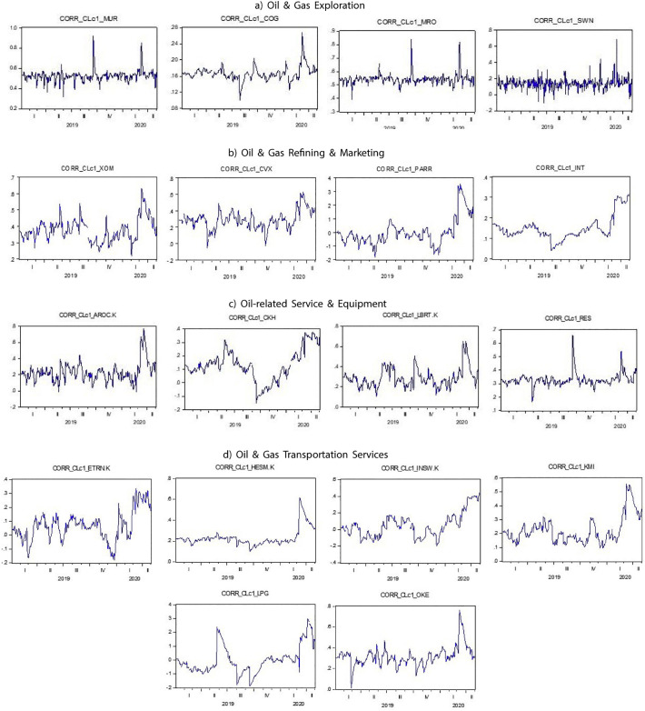
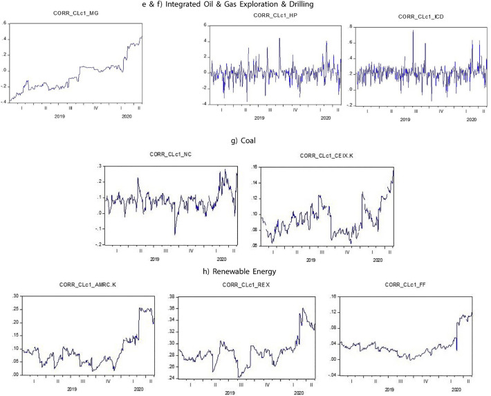
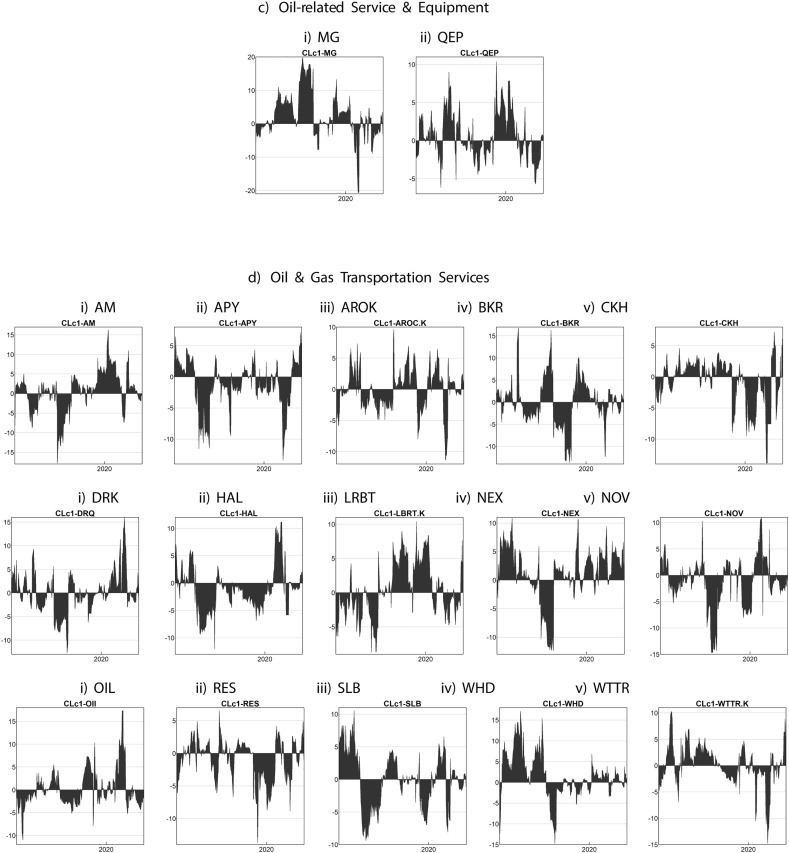
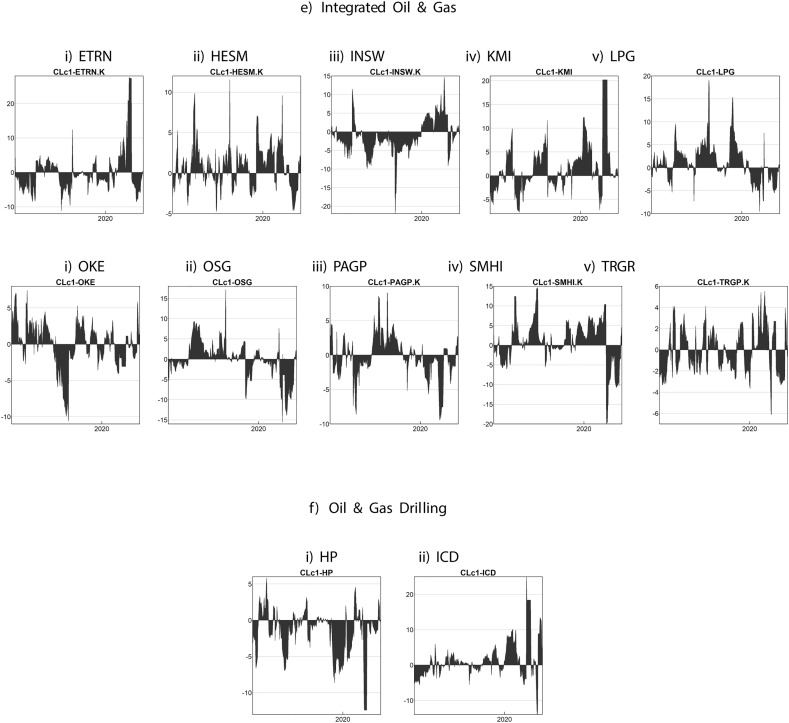
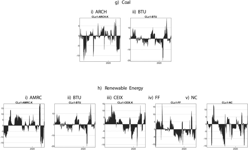
Fig. 4 illustrates our DCC-FIGARCH mapping of the dynamic correlations between WTI volatility and the volatility of a number of significant energy-related firms over our time period of 1 May 2019 and 12 May 2020. Firm-level illustrations are grouped by Thomson Reuters Business Classification (TRBC): oil and gas exploration, oil and gas refining and marketing, oil-related service and equipment, oil and gas transportation services, integrated oil and gas exploration and drilling, coal, and renewable energy. Examining Fig. 4, we see for many of the energy-related firms, spiking of dynamic correlation with WTI at differing points in our time period. However, for almost all the firms displayed there is a prominent spiking of dynamic correlation around 20 April 2020. This is particularly prominent for firms in Oil & Gas Exploration. For Renewable Energy, the focus of our study, we see a sharp rise on, or near 20 April 2020. However the spike in dynamic correlation is not nearly as narrow as for Oil & Gas Exploration.
Fig. 4.
Selected FIGARCH-calculated dynamic correlations between WTI volatility and the selected sectors as reported.
Note: The above data represents FIGARCH-calculated conditional correlation results based on hourly sectoral price volatility for the period March 2019 through May 2020. Data was obtained from Thomson Reuters Eikon.
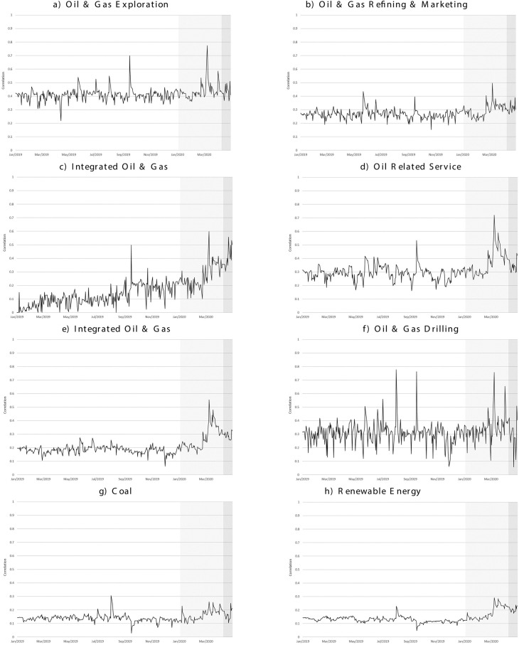
Examining more closely the relationships between WTI volatility and sectors, Fig. 5 illustrates our DCC-FIGARCH mapping of the dynamic correlations between WTI volatility and the aggregated volatility of relevant TRBC sectors over daily data. Examining Fig. 5, we see, for most sectors, a sharp spike in FIGARCH-calculated conditional correlation close to the time of negative WTI oil. Interestingly, we seen somewhat less of a spike for Coal and for Renewable Energy. This is one of the first signals of a clear behavioural separation between our selected TRBC sectors.7 One significant explanation for the behavioural differentials sourced within the renewable energy market surrounds the sharp, and unexpected drop in energy demand during the COVID-19 crisis, while renewables during the same period actually increased output. According to the International Energy Agency (IEA), global carbon dioxide emissions fell 8% during the initial stages of the pandemic, largely driven by an estimated reduction of 1.5% in annual energy demand per month of lock-down.
Fig. 5.
FIGARCH-calculated conditional correlation by sector, daily data (1 January 2019 through 1 May 2020).
Note: The above data represents FIGARCH-calculated conditional correlation results based on hourly sectoral price volatility for the period March 2019 through May 2020. Data was obtained from Thomson Reuters Eikon.
Observing the FIGARCH-calculated conditional correlation results in Table 3 , presenting time-varying evidence of interactions between markets during the denoted stages of the COVID-19 pandemic and the periods both before and after. Focusing on the mean values, in the period prior to COVID-19, there is a clear differential in the conditional correlations between WTI and energy related companies. For example, we observe that exploration companies present the largest estimated average correlation (+0.409), along with both the largest maximum and minimum estimates (+0.698 and +0.219 respectively). Behavioural differentials with respect to inter-sector correlations do not appear to vary substantially during the period surrounding the initial outbreak of a ‘mystery pneumonia’ in China during the period surrounding November and December 2019. However, we observe a broad increase in conditional correlations between each individual sector and the market for WTI in the period surrounding the official announcement by the WHO of the existence of an international pandemic. The largest increases in average values are identified in the sectors for integrated oil and gas, services and equipment, and transportation when compared to the pre-COVID-19 period. However, in the the aftermath of negative WTI prices, while further increases in conditional correlations are evident throughout our sample of energy sectors, integrated oil and gas companies experience the largest market interactions, where conditional correlations are estimated to have increased from an average of +0.111 in the period prior to the outbreak of COVID-19, to +0.453 in the period after the occurrence of negative oil. When focusing specifically on the markets for coal and renewable energy, we can observe a clear and significant increase in conditional correlations between the period before WHO confirmation of a pandemic and the period thereafter, however, these estimated values remain substantially below the other compared sectors. This evidence suggests, that while financial market panic ensued following the identification of COVID-19 increased market correlations, which has been previously identified as a signal of market stress (Hamao et al., 1990; Baig and Goldfajn, 1999; Forbes and Rigobon, 2002; Bae et al., 2003; Bekaert and Harvey, 2003), there remains clear separation in the behaviour of both the sectors for coal and renewable energy.
Table 3.
Average FIGARCH calculated conditional correlation by analysed sector.
| O&G explor. | O&G refin. | Integ. O&G | O&G S&Eq. | O&G trans. | O&G drill. | Coal | R.Energy | |
|---|---|---|---|---|---|---|---|---|
| Before COVID-19 | ||||||||
| Mean | 0.4094 | 0.2646 | 0.1112 | 0.2919 | 0.1856 | 0.3105 | 0.1386 | 0.1300 |
| Min | 0.2188 | 0.1527 | 0.0001 | 0.1605 | 0.1052 | 0.1191 | 0.0283 | 0.0483 |
| Max | 0.6986 | 0.4347 | 0.4986 | 0.5331 | 0.2742 | 0.7774 | 0.3064 | 0.2288 |
| Chinese-confirmed pneumonia | ||||||||
| Mean | 0.4045 | 0.2606 | 0.1792 | 0.2734 | 0.1601 | 0.2606 | 0.1245 | 0.1167 |
| Min | 0.3391 | 0.1851 | 0.0295 | 0.1896 | 0.0631 | 0.0615 | 0.0711 | 0.0852 |
| Max | 0.4638 | 0.3092 | 0.2706 | 0.3285 | 0.2111 | 0.3774 | 0.1499 | 0.1365 |
| WHO-confirmed COVID-19 | ||||||||
| Mean | 0.4375 | 0.2951 | 0.2763 | 0.3676 | 0.2736 | 0.3396 | 0.1628 | 0.1785 |
| Min | 0.3603 | 0.2104 | 0.1008 | 0.2428 | 0.1502 | 0.1053 | 0.0960 | 0.1148 |
| Max | 0.7740 | 0.4965 | 0.5989 | 0.7211 | 0.5542 | 0.7571 | 0.2603 | 0.2917 |
| Negative WTI prices and after | ||||||||
| Mean | 0.4416 | 0.3212 | 0.4526 | 0.3508 | 0.2901 | 0.2936 | 0.1733 | 0.2080 |
| Min | 0.3641 | 0.2783 | 0.3487 | 0.2956 | 0.2558 | 0.0574 | 0.1041 | 0.1761 |
| Max | 0.5107 | 0.3904 | 0.5580 | 0.4385 | 0.3330 | 0.5089 | 0.2494 | 0.2373 |
Note: The above data represents FIGARCH-calculated conditional correlation results based on hourly sectoral price volatility for the period March 2019 through May 2020. Data was obtained from Thomson Reuters Eikon. The conditional volatility of the above FIGARCH(1,d,1) model can be presented as: ht = ω + [1 − βL − (1 − ϕL)(1 − L)d]rt2 + βht−1 where L is a lag operator. The FIGARCH process then reduces to a GARCH process when d = 0. Further, the h-step ahead forecast of the FIGARCH(1,d,1) model is given by: ht+h = ω(1 − β)−1 + [1 − (1 − βL)−1(1 − ϕL)(1 − L)d]rt+h−12 where, if being used in the multivariate context, the same DCC approach is re-used with the same forecast functions for Qt+h and Rt+h. The multi-variate Student distribution is applied as the normality assumption of the innovations is rejected for each volatility series.
These initial results provide a number of interesting inter-sectoral behavioural differentials, some of which are largely of interest for those with commitment to broad portfolio diversification. The initiation of COVID-19, a largely unexpected black-swan event, has provided a broad example of the global fragility of our energy structures to economic and geopolitical shocks. The very fact that the COVID-19 pandemic has generated such widespread disruption generates rational fears with regards to the potential for further waves of the same pandemic, or perhaps fear of future pandemics from other sources. With regards to energy markets, a number of economic estimates have alarmed investors, with energy demand estimated to fall in excess of 6% for the full year of 2020, which is further estimated to be in excess of seven times the fall observed during the aftermath of the subprime collapse. However, renewable energy is now within the spectrum of government policy as many lobbyists have identified the COVID-19 pandemic as an opportunity to introduce a green-based recovery. Some of the key driving forces of such opportunistic policy have surrounded the sustained reduction in demand for oil, driven by a sharp fall in demand for manufacturing (down over 50% in some cases), aviation (estimated to have fallen over 90% worldwide) and a range of other energy-intensive processes. Demand for coal has fallen approximately 8%, while its usage to generate electricity in India, China, the EU and US has fallen substantially as gas prices have fallen and provided a cheap substitute, while the burning of coal has become socially untenable. Gas consumption fell for the first time since 2009 presenting an unexpected reversal, driven for the most-part by a sharp reduction in reduced power generation. Such positive effects from renewable energy could have potentially being more influential through broad improvements in the re-supply of power into electricity grids, to improve upon the estimated 40% of global electricity production from renewable sources. These factors will be central to maintain a pathway towards achieving the ambitious targets in the Paris climate agreement.
4.2. Directional volatility spillovers
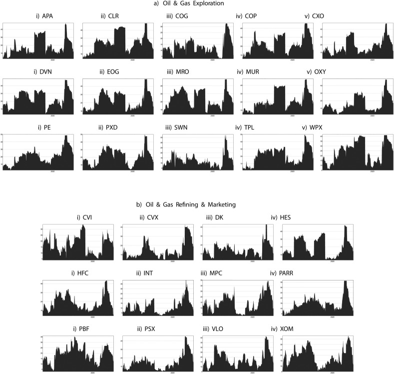
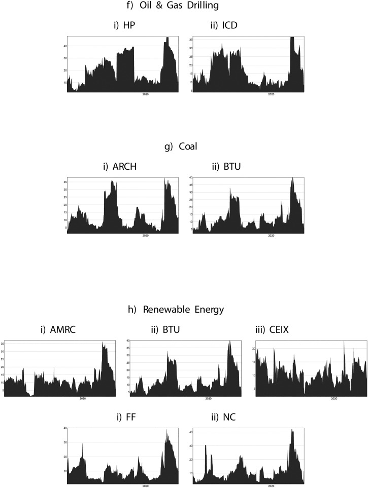
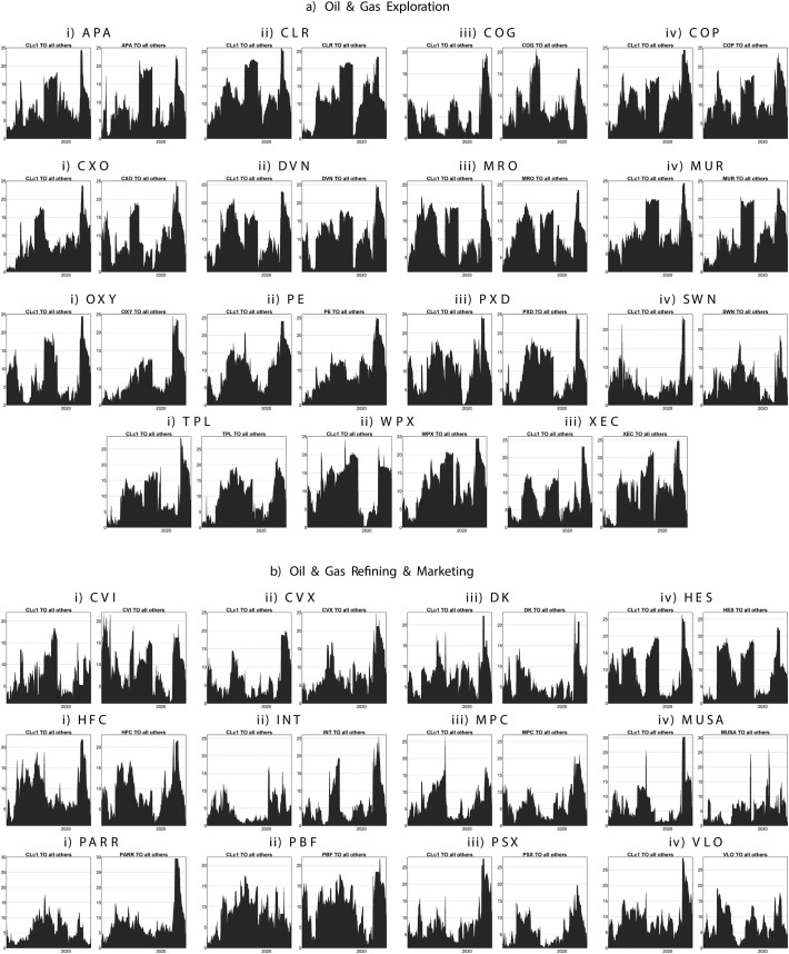
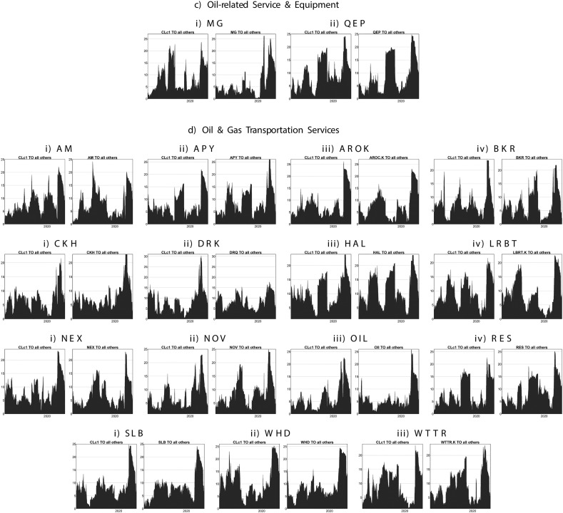
Fig. 6 illustrates our investigation of Diebold and Yilmaz (2009) spillover from WTI oil to a number of significant energy-related firms over our time period of 1 May 2019 and 12 May 2020.As in previous figures, firm-level illustrations are grouped by Thomson Reuters Business Classification. Fig. 7 shows, alternatively, the total directional spillover of WTI to energy firms and the directional spillover of firms to WTI. We see for both Fig. 6, Fig. 7 a dramatic spike on 20 April 2020, as WTI went negative. This suggests that the time of WTI negative pricing was a time of extraordinary bi-directional spillovers between WTI and energy-related companies of all types. It is not surprising that there would be extremely heightened bi-directional interactions with oil by energy companies of all types during a time of an extraordinary fall in WTI prices.
Fig. 6.
Total directional volatility spillovers from WTI onto each analysed sector, absolute returns, 50-day window.
Note: The above table represents the total directional volatility spillovers from WTI upon each stated energy sector. To examine spillovers in the volatility of WTI during the outbreak of the COVID-19 pandemic and the subsequent effects of negative oil prices, and the effects of each event on energy-companies in the US, we apply the generalised version of the spillover index proposed by Diebold and Yilmaz (2009), and which builds on the vector autoregressive (VAR) models developed by Sims (1980).
Fig. 7.
Total directional volatility spillovers to WTI from each analysed sector, absolute returns, 50-day window.
Note: The above table represents the total directional volatility spillovers from WTI upon each stated energy sector. To examine spillovers in the volatility of WTI during the outbreak of the COVID-19 pandemic and the subsequent effects of negative oil prices, and the effects of each event on energy-companies in the US, we apply the generalised version of the spillover index proposed by Diebold and Yilmaz (2009), and which builds on the vector autoregressive (VAR) models developed by Sims (1980).
In Table 4 , we identify the net directional connectedness by selected stocks and WTI. Relationships are presented for the periods both before and after the occurence of negative WTI prices. Further evidence of elevated market correlations during the COVID-19 period is identified. This signals the presence of broad contagion of investor fears within the oil and gas industries. Some of the largest increases are found to have occurred in the oil and gas refining and marketing sector and the oil and gas services and equipment sector. One of the most interesting results occurs for the market for renewable energies, where we evidence the decoupling of stocks related to green energy.
Table 4.
Net directional connectedness, by stock.
| Ticker | CLc1 | Stock | Conn#. | Stock | CLc1 |
|---|---|---|---|---|---|
| a) Oil & gas exploration | |||||
| CLR | 24.96 | 75.04 | +2.95 | 77.99 | 22.01 |
| APA | 21.35 | 78.65 | +2.36 | 81.01 | 18.99 |
| MRO | 25.18 | 74.82 | +1.77 | 76.59 | 23.41 |
| TPL | 28.27 | 71.73 | +10.12 | 81.86 | 18.14 |
| EQT | 15.28 | 84.72 | +2.89 | 87.61 | 12.39 |
| WPX | 21.32 | 78.68 | +12.37 | 66.31 | 33.69 |
| EOG | 21.65 | 78.35 | −1.93 | 76.42 | 23.58 |
| OXY | 20.96 | 79.04 | −2.07 | 76.97 | 23.03 |
| CXO | 14.38 | 85.62 | −1.00 | 75.78 | 24.22 |
| CNX | 17.65 | 82.35 | +4.66 | 87.02 | 12.98 |
| b) Oil & gas refining & marketing | |||||
| PSX | 30.36 | 69.64 | +15.06 | 84.70 | 15.30 |
| VLO | 26.06 | 73.94 | +9.12 | 83.07 | 16.93 |
| HES | 23.03 | 76.97 | +0.46 | 77.44 | 22.56 |
| MUSA | 14.33 | 85.67 | +9.46 | 95.13 | 4.87 |
| DK | 20.60 | 79.40 | +2.98 | 82.38 | 17.62 |
| INT | 7.82 | 92.18 | +14.72 | 77.46 | 22.54 |
| PARR | 9.21 | 90.79 | +19.47 | 71.32 | 28.68 |
| c) Oil & gas services & equipment | |||||
| QEP | 23.09 | 76.91 | +11.44 | 65.47 | 34.53 |
| MG | 16.31 | 83.69 | +16.56 | 67.14 | 32.86 |
| d) Oil & gas transportation services | |||||
| SLB | 22.70 | 77.30 | −2.52 | 74.77 | 25.23 |
| BKR | 12.58 | 87.42 | −1.74 | 85.67 | 14.33 |
| WHD | 30.46 | 69.54 | +1.94 | 71.49 | 28.51 |
| DRQ | 17.23 | 82.77 | +1.38 | 84.15 | 15.85 |
| AROC | 27.02 | 72.98 | +3.48 | 76.46 | 23.54 |
| RES | 25.34 | 74.66 | +10.80 | 85.46 | 14.54 |
| APY | 26.39 | 73.61 | +1.13 | 74.74 | 25.26 |
| LBRT | 29.97 | 70.03 | +5.02 | 75.05 | 24.95 |
| WTTR | 26.23 | 73.77 | +1.10 | 74.87 | 25.13 |
| NEX | 24.39 | 75.61 | +3.54 | 79.16 | 20.84 |
| e) Integrated oil & gas | |||||
| WMB | 8.32 | 91.68 | +15.16 | 76.52 | 23.48 |
| OKE | 18.17 | 81.83 | +15.11 | 66.71 | 33.29 |
| ETRN | 9.73 | 90.27 | −5.01 | 85.27 | 14.73 |
| LPG | 13.57 | 86.43 | −3.58 | 82.86 | 17.14 |
| f) Oil & gas drilling | |||||
| HP | 20.78 | 79.22 | −6.03 | 73.18 | 26.82 |
| ICD | 22.46 | 77.54 | +12.23 | 89.78 | 10.22 |
| g) Coal | |||||
| NC | 16.60 | 83.40 | +1.00 | 84.39 | 15.61 |
| CEIX | 19.99 | 80.01 | +1.70 | 81.71 | 18.29 |
| CTRA | 19.83 | 80.17 | +2.16 | 82.34 | 17.66 |
| h) Renewable energy | |||||
| AMRC | 3.45 | 96.55 | −11.63 | 84.92 | 15.08 |
| FF | 4.81 | 95.19 | −9.40 | 85.79 | 14.21 |
Note: # represents the estimate of net directional connectedness. For brevity and presentation purposes, only significant results at the 1% level that are not equal to zero are presented. Further results at varying time-frequencies and variation of methodological structure are available from the authors on request. The above analysis is conducted using the net pairwise volatility spillover can therefore be presented as: . The net pairwise volatility spillovers between markets i and j is therefore calculated using Eq. (15), defined simply as the difference between the gross volatility shocks transmitted from variable i to j while considering the shocks transmitted from j to i.
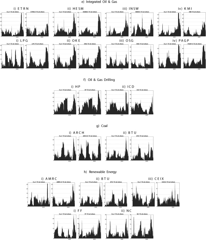
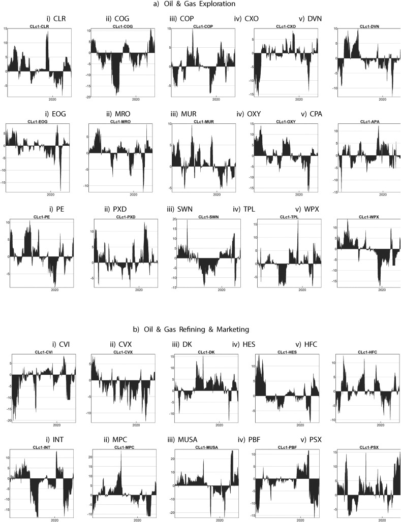
Further evidence of a sectoral basis is illustrated in Table 5 , where broad differentials are shown in the behaviour of the sectors for coal and renewable energy (−1.19 and −5.51 respectively) in the period after the outbreak of the COVID-19 pandemic and subsequent negative oil pricing event. Individual net pairwise directional volatility spillovers are presented in Fig. 8 . Our results are consistent with international lock-downs leading to a sharp drop in demand for electricity, concomitant with, however, a sharp increase in demand for renewable energy. In contrast, demand for coal fell quite acutely. The COVID-19 pandemic created a number of substantial queries with regards to how long exactly lock-downs would be imposed and how long and deep a subsequent COVID-19 induced recession would hinder electricity demand?
Table 5.
Net directional connectedness, by sector.
| Sector | Net directional connectedness |
Directional flow from CLC1 market |
||||
|---|---|---|---|---|---|---|
| Average | Minimum | Maximum | Average | Minimum | Maximum | |
| a) Oil & gas exploration | 1.39 | −3.94 | 12.37 | 79.83 | 71.73 | 88.90 |
| b) Oil & gas refining & marketing | 3.59 | −7.74 | 19.47 | 81.52 | 69.64 | 92.18 |
| c) Oil & gas services & equipment | 1.40 | −1.14 | 16.56 | 80.30 | 76.91 | 83.69 |
| d) Oil & gas transportation services | 2.08 | −2.52 | 10.80 | 76.54 | 69.54 | 87.42 |
| e) Integrated oil & gas | 1.85 | −5.01 | 15.16 | 83.45 | 74.98 | 91.68 |
| f) Oil & gas drilling | 3.10 | −6.03 | 12.23 | 78.38 | 77.54 | 79.22 |
| g) Coal | −1.19 | −7.95 | 12.16 | 82.54 | 80.01 | 86.97 |
| h) Renewable energy | −5.51 | −9.40 | 6.63 | 91.89 | 83.94 | 96.55 |
Note: The above table represents the net directional connectedness by stated energy sector. To examine spillovers in the volatility of WTI during the outbreak of the COVID-19 pandemic and the subsequent effects of negative oil prices, and the effects of each event on energy-companies in the US, we apply the generalised version of the spillover index proposed by Diebold and Yilmaz (2009), and which builds on the vector autoregressive (VAR) models developed by Sims (1980). The above analysis is conducted using the net pairwise volatility spillover can therefore be presented as: . The net pairwise volatility spillovers between markets i and j is therefore calculated using Eq. (15), defined simply as the difference between the gross volatility shocks transmitted from variable i to j while considering the shocks transmitted from j to i.
Fig. 8.
Net pairwise directional volatility spillovers, absolute returns, 50-day window.
Note: The above table represents the net pairwise directional volatility spillovers by stated energy sector. To examine spillovers in the volatility of WTI during the outbreak of the COVID-19 pandemic and the subsequent effects of negative oil prices, and the effects of each event on energy-companies in the US, we apply the generalised version of the spillover index proposed by Diebold and Yilmaz (2009), and which builds on the vector autoregressive (VAR) models developed by Sims (1980).
Differentials in effects experienced within coal and renewable energy sectors during COVID-19 are likely signals of pronounced changes in forecasted energy needs. As the effects of the coronavirus spread, electricity demand fell8 by approximately 2.5%. Some might have expected to have been reflected in an even distribution of energy reduction, both by type and by sector. However, demand for coal fell in excess of 10%, while demand for renewable energy actually increased by 3%. This latter result is consistent with signalling a substantial shift towards low-carbon energy sources. These effects were likely driven by the price of fuel. However, are these price-driven results due to Saudi Arabia opening oil supplies? Or, alternatively, are these results caused by a strong downward turn in world expectations for energy use? These two interpretations are reflected in our two alternative hypotheses presented earlier.
In later sections of this paper we investigate these alternatives more closely by examining directional spillovers from WTI oil to both coal and renewables separately for our three sample periods: Chinese COVID, WHO COVID, and Negative Oil. Both explanations are consistent with renewables gaining in general, and gaining differentially on coal during declining global energy demand forecasts. Coal might gain from negative oil as lower oil prices are known to be an existential threat to the US fracking industry. But coal also loses generally to lower energy prices.9
But there is another question: How did, and how does, coal react to sharply downward re-estimation of future global energy needs? Will the composition of global energy be fundamentally altered by events so extreme to bring about negative oil prices? We expect coal and renewable to negatively co-move in “normal times”, as confirmed in previous literature and as consistent with the periods of our study that are not negative WTI. However, during our negative WTI period, did coal fall as much as would be expected from simply a sharp reduction in energy prices? Or was there a mitigating effect of due to changing investor expectations for global energy use and concomitant reshaping of which industries would be best positioned to supply a downward forecast of future needs? We next examine directional spillovers in an effort to answer these important questions.
Table 6 perhaps shows most clearly the crux of our results. Examining Table 6, we see an extraordinary change during the time of negative WTI event with respect to the reaction of industries in coal and renewables to WTI. As seen in Table 6, we divide our results regarding directional spillovers into three time categories: 1) an early time in the evolution of COVID-19, when it was largely limited to China (Chinese COVID); the time when COVID-19 had broadened to affect most of the globe, but preceding the period just before 20 April 2020, the time of negative WTI prices (WHO COVID); and the time surrounding the negative oil event (Negative WTI). With the exception of firms in the Integrated Oil & Gas sector, other sectors received generally negatively correlated spillovers from WTI during the Chinese COVID and WHO COVID periods. These spillovers were generally quite moderate in magnitude, the largest in absolute terms being a − 2.19 value for Oil & Gas Refining & Marketing during the time of Chinese COVID.
Table 6.
Average directional spillover, by sector.
| Sector | Chinese COVID | WHO COVID | Negative WTI |
|---|---|---|---|
| a) Oil & gas exploration | −1.76 | −2.10 | +4.83 |
| b) Oil & gas refining & marketing | −2.19 | −1.83 | +3.91 |
| c) Oil & gas services & equipment | −0.59 | −0.14 | +1.75 |
| d) Oil & gas transportation services | −0.72 | −0.18 | +1.30 |
| e) Integrated oil & gas | +1.48 | +1.26 | −0.25 |
| f) Oil & gas drilling | −1.63 | −1.49 | +5.71 |
| g) Coal | −0.95 | −0.40 | −4.96 |
| h) Renewable energy | −0.38 | −0.17 | −9.96 |
Note: The above table represents the average directional connectedness by stated energy sector. To examine spillovers in the volatility of WTI during the outbreak of the COVID-19 pandemic and the subsequent effects of negative oil prices, and the effects of each event on energy-companies in the US, we apply the generalised version of the spillover index proposed by Diebold and Yilmaz (2009), and which builds on the vector autoregressive (VAR) models developed by Sims (1980). The above analysis is conducted using the net pairwise volatility spillover can therefore be presented as: . The net pairwise volatility spillovers between markets i and j is therefore calculated using Eq. (15), defined simply as the difference between the gross volatility shocks transmitted from variable i to j while considering the shocks transmitted from j to i.
However, during the Negative WTI period, Oil & Gas Exploration and Oil & Gas Refining & Marketing jumped to values of +4.83 and + 3.91 respectively. However, the Coal sector and the Renewable Energy sector both spiked in absolute terms to −4.96 and − 9.96 respectively. Only the sectors Coal and Renewable Energy had positive values during the time of negative WTI. The magnitude of the spillover to the renewable sector of −9.96 is approximately double the magnitude of any other spillovers in any of the three periods.
Our results, specifically for the narrow period around negative WTI, stand in a stark contrast to a number of articles of recent years that find renewables falling and gaining with oil (such as the works of Apergis and Payne, 2014; Ferrer et al., 2018; Khan et al., 2017; Reboredo, 2015, Reboredo et al., 2017; and Sadorsky, 2009, Sadorsky, 2012a, Sadorsky, 2012b). However, unlike these papers, we test this interaction under the condition of an unprecedented global downturn. Of additional interest is the extreme suddenness of the bi-directional spillovers of the firms in our sample. Our figures consistently illustrate levels of spillover having an extreme and narrow spiking of spillovers centred around April 20, 2020. These results will be of interest to those interested in contagion in general beyond the interactions of energy firms. As Yarovaya et al. (2020) suggest, during and post COVID-19 we may see a quickening of co-movements brought about by heightened public and media attention based on the perception of economic frailty and widespread vulnerability.
5. Conclusions
The unprecedented fall to negative values of WTI oil prices in April 2020, occurring during the unprecedented economic turmoil surrounding the COVID-19 pandemic, compels examination of the co-movements and spillovers among energy-related companies during this time. Indeed, some are even suggesting a reassessment of all forms of market contagion for a COVID-19 and post-COVID-19 world.
The COVID-19 pandemic by itself provides an unprecedented background to re-examine spillovers between energy firms during a very sharp downturn in short-term and long-term expectations of global energy use. Concomitantly, on April 20, 2020 was the extraordinary, sudden, and brief occurrence of negative oil prices on one of the world's primary markets. During the first portion of April 2020, oil traders were contending with broadly attempting to quantify the severity of COVID-19 and its influence on worldwide demand for oil; as well as assessing broad oil-related geopolitical issues related to the relationship between Saudi Arabia and Russia. One result of the confluence of COVID-19's impact on global energy demand and geopolitical tensions between oil producers was the dramatic fall of WTI oil to negative values. Certainly, there is a pressing need of a thorough investigation of the co-movements in returns, and volatility among energy-related firms of many energy industries during surrounding this unprecedented set of circumstances in the energy markets.
We test for the existence of volatility spillovers and co-movements among energy-focused corporations during the outbreak of the COVID-19 pandemic, inclusive of the April 2020 events where West Texas Intermediate (WTI) oil future prices became negative. Employing the spillover index of Diebold and Yilmaz (2009); as well as developing a DCC-FIGARCH conditional correlation framework and using estimated spillover indices built on a generalised vector autoregressive framework in which forecast-error variance decompositions are invariant to the variable ordering, we examine the sectoral transmission mechanisms of volatility shocks and contagion throughout the energy sector. Among several results, we find positive and economically meaningful spillovers from falling oil to both renewables and coal for the very specific period surrounding the time of WTI falling to negative values. We interpret our results as investors seeing the extraordinary fall in WTI as due to a sharp drop in global demand, rather than because of a sudden increase in oil supply. While investors saw the US fracking industry losing to coal, they also viewed renewables as more reliable to generate long-term supply.
Footnotes
Signals of forthcoming issues had been evident in Canada on 19 April 2020, when steam-assisted gravity drainage projects, that heat seams of bitumen and account for nearly half of Canadian-oil sands production were cut by ConocoPhillips, as a signal that Canada's oil economy was bearing the brunt of output cuts in the midst of low prices, and deeper reductions in production caused substantial restructure as Canadian oil prices went negative. A similar, regional issue occurred with natural gas prices in Western Canada that turned negative in 2017, due to a number of pipeline maintenance issues due to storage options that then created a rapid accumulation of supply. The influence of these broad risks upon the US oil & gas sector is a centrally positioned question within current literature, particularly with the substantial risks of repeated pandemics remaining in a state of elevation and associated risks for both traders and regulators when considering the sector's transition to a state of improved long-term environmental sustainability (CBC News, Canada, 26 October 2017).
See also Krause and Tse (2013) for exchange traded funds and Antonakakis and Vergos (2013); Claeys and Vašíček (2014) for bond markets.
Research relating to interactions with negative pricing behaviour is generally quite limited. Fanone et al. (2013) investigate the case of negative day-ahead electricity prices, presenting a non-Gaussian process that is found to be able to generate extreme positive and negative spikes. Valitov (2019) find such events of negative electricity prices lead to a decrease in risk premia when compared to the period of a positive price regime.
He et al. (2010) find that daily WTI highs and lows are cointegrated, with the error correction term being closely approximated by the daily price range.
For brevity, only hourly analyses are presented in this version. Variation of frequency presented little differential in results. The results of additional analyses are available from the authors upon request. The starting point of our data is dictated by availability from data suppliers. Daily price data presents the largest time-span, however, 1-min data presents the largest number of observations.
We further experimented with alternative measures of volatility, such as conditional volatility. Further, we proceeded to prepared our analysis based on the elimination of public holidays and further windsorisation at the 1% level of illiquid trading conditions. However, our results remained qualitatively similar to those presented.
For more detail, appendix Table A2, lists Hurst exponents by company and sector. Figs. A1 and A2 show sensitivities to respectively VAR lag structure and forecast horizon
The associated IEA electricity Flagship report, released in April 2020, is available here.
Throughout April and May 2020, renewable energy out-generated coal, with IHS Markit stating that for producers such as PJM Interconnection LLC, the volume of coal generated energy fell by 40%, while the generation of solar energy increased by 45%. It should be noted that the use of coal has been in steady decline since 2010 In late 2019, the use of coal for electricity production fell to its lowest level in over forty years.
Supplementary data to this article can be found online at https://doi.org/10.1016/j.eneco.2020.104978.
Appendix A. Supplementary data
Appendix 1
Supplementary data
References
- Aggarwal R., Akhigbe A., Mohanty S.K. Oil price shocks and transportation firm asset prices. Energy Econ. 2012;34(5):1370–1379. [Google Scholar]
- Antonakakis N., Vergos K. Sovereign bond yield spillovers in the Eurozone during the financial and debt crisis. J. Int. Financ. Mark. Inst. Money. 2013;26(1):258–272. [Google Scholar]
- Antonakakis N., Chatziantoniou I., Filis G. Dynamic spillovers of oil price shocks and economic policy uncertainty. Energy Econ. 2014;44:433–447. [Google Scholar]
- Antonakakis N., Cunado J., Filis G., Gabauer D., Perez de Gracia F. Oil volatility, oil and gas firms and portfolio diversification. Energy Econ. 2018;70:499–515. [Google Scholar]
- Apergis N., Payne J.E. Renewable energy, output, CO2 emissions, and fossil fuel prices in Central America: evidence from a nonlinear panel smooth transition vector error correction model. Energy Econ. 2014;42:226–232. [Google Scholar]
- Arouri M., Lahiani A., Lévy A., Nguyen D. Forecasting the conditional volatility of oil spot and futures prices with structural breaks and long memory models. Energy Econ. 2012;34(1):283–293. [Google Scholar]
- Awartani B., Maghyereh A. Dynamic spillovers between oil and stock markets in the Gulf Cooperation Council Countries. Energy Econ. 2013;36:28–42. [Google Scholar]
- Bae K.-H., Karolyi G.A., Stulz R.M. A new approach to measuring financial contagion. Rev. Financ. Stud. 2003;16(3):717–763. [Google Scholar]
- Baig T., Goldfajn I. Financial market contagion in the asian crisis. IMF Staff. Pap. 1999;46(2):167–195. [Google Scholar]
- Baillie R.T., Chung C.-F., Tieslau M.A. Analysing inflation by the fractionally integrated ARFIMA–GARCH model. J. Appl. Econ. 1996;11(1):23–40. [Google Scholar]
- Balcilar M., Gupta R., Wohar M. Common cycles and common trends in the stock and oil markets: evidence from more than 150 years of data. Energy Econ. 2017;61:72–86. [Google Scholar]
- Beine M., Capelle-Blancard G., Raymond H. International nonlinear causality between stock markets. Eur. J. Financ. 2008;14(8):663–686. [Google Scholar]
- Bekaert G., Harvey C.R. National Bureau of Economic Research; 2003. Market Integration and Contagion. Technical report. [Google Scholar]
- Bekiros S., Shahzad S., Arreola-Hernandez J., Ur Rehman M. Directional predictability and time-varying spillovers between stock markets and economic cycles. Econ. Model. 2018;69:301–312. [Google Scholar]
- Bentes S. Measuring persistence in stock market volatility using the FIGARCH approach. Physica A. 2014;408:190–197. [Google Scholar]
- Boyer M.M., Filion D. Common and fundamental factors in stock returns of Canadian oil and gas companies. Energy Econ. 2007;29(3):428–453. [Google Scholar]
- Claeys P., Vašíček B. Measuring bilateral spillover and testing contagion on sovereign bond markets in Europe. J. Bank. Financ. 2014;46(1):151–165. [Google Scholar]
- Cong R.-G., Wei Y.-M., Jiao J.-L., Fan Y. Relationships between oil price shocks and stock market: an empirical analysis from China. Energy Policy. 2008;36(9):3544–3553. [Google Scholar]
- Conlon T., Corbet S., McGee R.J. Research in International Business and Finance. 2020. Are cryptocurrencies a safe haven for equity markets? An international perspective from the COVID-19 pandemic; p. 101248. [DOI] [PMC free article] [PubMed] [Google Scholar]
- Cont R. 2001. Empirical Properties of Asset Returns: Stylized Facts and Statistical Issues. [Google Scholar]
- Corbet S., Hou G., Hu Y., Larkin C.J., Oxley L. Any port in a storm: cryptocurrency safe-havens during the COVID-19 pandemic. Econ. Lett. 2020 doi: 10.1016/j.econlet.2020.109377. (forthcoming) [DOI] [PMC free article] [PubMed] [Google Scholar]
- Corbet S., Hou G., Hu Y., Oxley L. 2020. The Influence of the COVID-19 Pandemic on Asset-price Discovery: Testing the Case of Chinese Informational Asymmetry. (Available at SSRN 3623274) [DOI] [PMC free article] [PubMed] [Google Scholar]
- Davidson J. Moment and memory properties of linear conditional heteroscedasticity models, and a new model. J. Bus. Econ. Stat. 2004;22(1):16–29. [Google Scholar]
- Diebold F.X., Inoue A. Long memory and regime switching. J. Econ. 2001;105(1):131–159. [Google Scholar]
- Diebold F.X., Yilmaz K. Measuring financial asset return and volatility spillovers, with application to global equity markets. Econ. J. 2009;119(534):158–171. [Google Scholar]
- Diebold F.X., Yilmaz K. Better to give than to receive: predictive directional measurement of volatility spillovers. Int. J. Forecast. 2012;28(1):57–66. [Google Scholar]
- Ding Z., Granger C.W., Engle R.F. A long memory property of stock market returns and a new model. J. Empir. Financ. 1993;1(1):83–106. [Google Scholar]
- Du L., He Y. Extreme risk spillovers between crude oil and stock markets. Energy Econ. 2015;51:455–465. [Google Scholar]
- Engle R. Dynamic conditional correlation: a simple class of multivariate generalized autoregressive conditional heteroskedasticity models. J. Bus. Econ. Stat. 2002;20(3):339–350. [Google Scholar]
- Fanone E., Gamba A., Prokopczuk M. The case of negative day-ahead electricity prices. Energy Econ. 2013;35:22–34. [Google Scholar]
- Ferrer R., Shahzad S.J.H., López R., Jareño F. Time and frequency dynamics of connectedness between renewable energy stocks and crude oil prices. Energy Econ. 2018;76:1–20. [Google Scholar]
- Forbes K.J., Rigobon R. No contagion, only interdependence: measuring stock market comovements. J. Financ. 2002;57(5):2223–2261. [Google Scholar]
- Goodell J.W. COVID-19 and finance: agendas for future research. Financ. Res. Lett. 2020;101512 doi: 10.1016/j.frl.2020.101512. [DOI] [PMC free article] [PubMed] [Google Scholar]
- Hamao Y., Masulis R.W., Ng V. Correlations in price changes and volatility across international stock markets. Rev. Financ. Stud. 1990;3(2):281–307. [Google Scholar]
- Harris R.D., Nguyen A. Long memory conditional volatility and asset allocation. Int. J. Forecast. 2013;29(2):258–273. [Google Scholar]
- He A., Kwok J., Wan A. An empirical model of daily highs and lows of West Texas intermediate crude oil prices. Energy Econ. 2010;32(6):1499–1506. [Google Scholar]
- Henriques I., Sadorsky P. Oil prices and the stock prices of alternative energy companies. Energy Econ. 2008;30(3):998–1010. [Google Scholar]
- Ho K.-Y., Shi Y., Zhang Z. How does news sentiment impact asset volatility? Evidence from long memory and regime-switching approaches. N. Am. J. Econ. Financ. 2013;26:436–456. [Google Scholar]
- Huang R.D., Masulis R.W., Stoll H.R. Energy shocks and financial markets. J. Futur. Mark. 1996;16(1):1–27. [Google Scholar]
- Jones C.M., Kaul G. Oil and the stock markets. J. Financ. 1996;51(2):463–491. [Google Scholar]
- Kang S., Cho H.-G., Yoon S.-M. Modeling sudden volatility changes: evidence from Japanese and Korean stock markets. Physica A. 2009;388(17):3543–3550. [Google Scholar]
- Kang S., Cheong C., Yoon S.-M. Long memory volatility in chinese stock markets. Physica A. 2010;389(7):1425–1433. [Google Scholar]
- Kapetanios G. Unit-root testing against the alternative hypothesis of up to m structural breaks. J. Time Ser. Anal. 2005;26(1):123–133. [Google Scholar]
- Khan M.I., Yasmeen T., Shakoor A., Khan N.B., Muhammad R. 2014 oil plunge: causes and impacts on renewable energy. Renew. Sust. Energ. Rev. 2017;68:609–622. [Google Scholar]
- Krause T., Tse Y. Volatility and return spillovers in Canadian and U.S. industry ETFs. Int. Rev. Econ. Financ. 2013;25:244–259. [Google Scholar]
- Kumar S., Managi S., Matsuda A. Stock prices of clean energy firms, oil and carbon markets: a vector autoregressive analysis. Energy Econ. 2012;34(1):215–226. [Google Scholar]
- Liow K. Volatility spillover dynamics and relationship across G7 financial markets. N. Am. J. Econ. Financ. 2015;33:328–365. [Google Scholar]
- Maghyereh A., Awartani B., Bouri E. The directional volatility connectedness between crude oil and equity markets: new evidence from implied volatility indexes. Energy Econ. 2016;57:78–93. [Google Scholar]
- Maghyereh A.I., Awartani B., Abdoh H. The co-movement between oil and clean energy stocks: a wavelet-based analysis of horizon associations. Energy. 2019;169:895–913. [Google Scholar]
- Miller J.I., Ratti R.A. Crude oil and stock markets: stability, instability, and bubbles. Energy Econ. 2009;31(4):559–568. [Google Scholar]
- Otranto E. Capturing the spillover effect with multiplicative error models. Commun. Stat. Theory Methods. 2015;44(15):3173–3191. [Google Scholar]
- Park J., Ratti R.A. Oil price shocks and stock markets in the us and 13 european countries. Energy Econ. 2008;30(5):2587–2608. [Google Scholar]
- Phan D.H.B., Sharma S.S., Narayan P.K. Intraday volatility interaction between the crude oil and equity markets. J. Int. Financ. Mark. Inst. Money. 2016;40:1–13. [Google Scholar]
- Reboredo J.C. Is there dependence and systemic risk between oil and renewable energy stock prices? Energy Econ. 2015;48:32–45. [Google Scholar]
- Reboredo J.C., Rivera-Castro M.A., Ugolini A. Wavelet-based test of co-movement and causality between oil and renewable energy stock prices. Energy Econ. 2017;61:241–252. [Google Scholar]
- Sadorsky P. Renewable energy consumption, CO2 emissions and oil prices in the G7 countries. Energy Econ. 2009;31(3):456–462. [Google Scholar]
- Sadorsky P. Correlations and volatility spillovers between oil prices and the stock prices of clean energy and technology companies. Energy Econ. 2012;34(1):248–255. [Google Scholar]
- Sadorsky P. Modeling renewable energy company risk. Energy Policy. 2012;40:39–48. [Google Scholar]
- Salisu A., Oloko T. Modelling oil price-US stock nexus: a VARMA-BEKK-AGARCH approach. Energy Econ. 2015;50:1–12. [Google Scholar]
- Shahzad S., Ferrer R., Ballester L., Umar Z. Risk transmission between islamic and conventional stock markets: a return and volatility spillover analysis. Int. Rev. Financ. Anal. 2017;52:9–26. [Google Scholar]
- Sims C.A. Macroeconomics and reality. Econometrica. 1980:1–48. [Google Scholar]
- Valitov N. Risk premia in the german day-ahead electricity market revisited: the impact of negative prices. Energy Econ. 2019;82:70–77. [Google Scholar]
- Xiarchos I.M., Burnett J.W. Dynamic volatility spillovers between agricultural and energy commodities. J. Agric. Appl. Econ. 2018;50(3):291–318. [Google Scholar]
- Xu W., Ma F., Chen W., Zhang B. Asymmetric volatility spillovers between oil and stock markets: evidence from China and the United States. Energy Econ. 2019;80:310–320. [Google Scholar]
- Yang L. Connectedness of economic policy uncertainty and oil price shocks in a time domain perspective. Energy Econ. 2019;80:219–233. [Google Scholar]
- Yang K., Chen L., Tian F. Realized volatility forecast of stock index under structural breaks. J. Forecast. 2015;34(1):57–82. [Google Scholar]
- Yarovaya L., Brzeszczynski J., Goodell J.W., Lucey B.M., Lau C.K. 2020. Rethinking Financial Contagion: Information Transmission Mechanism During the COVID-19 Pandemic. (Available at SSRN 3602973) [Google Scholar]
- Zhang D. Oil shocks and stock markets revisited: measuring connectedness from a global perspective. Energy Econ. 2017;62:323–333. [Google Scholar]
Associated Data
This section collects any data citations, data availability statements, or supplementary materials included in this article.
Supplementary Materials
Appendix 1
Supplementary data


