Abstract
The Wiener-Granger causality test is used to predict future experimental results from past observations in a purely mathematical way. For instance, in many scientific papers this test has been used to study the causality relations in the case of neuronal activities. Albeit some papers reported repeatedly about problems or open questions related to the application of the Granger causality test on biological systems, these criticisms were always related to some kind of assumptions to be made before the test's application. In our paper instead we investigate the Granger method itself, making use exclusively of fundamental mathematical tools like Fourier transformation and differential calculus. We find that the ARMA method reconstructs any time series from any time series, regardless of their properties, and that the quality of the reconstruction is given by the properties of the Fourier transform. In literature several definitions of “causality” have been proposed in order to maintain the idea that the Granger test might be able to predict future events and prove causality between time series. We find instead that not even the most fundamental requirement underlying any possible definition of causality is met by the Granger causality test. No matter of the details, any definition of causality should refer to the prediction of the future from the past; instead by inverting the time series we find that Granger also allows one to “predict” the past from the future.
Keywords: Applied mathematics, Mathematical biosciences, Neuroscience, Wiener-Granger, Causality, Linear regression
Applied mathematics; Mathematical biosciences; Neuroscience; Wiener-Granger; Causality; Linear regression
1. Introduction
In 1969 Granger [1] (who was awarded the Nobel Memorial Prize in Economic Sciences in 2003) suggested to define a causality relation by means of a mathematical procedure between variables without any knowledge about their underlying mechanisms; in 1980 [2] he developed the first mathematical formulation of causality, applying this method for the first time in economics. Later on his formulation was abandoned in that field.
Nowadays, however, it is gaining increasing importance in other sectors, for example in neuroscience [3] to investigate functional neural systems at scales of organization from the cellular level [4], [5], [6] to the whole-brain network activity [7]. Despite its popularity, several studies, even in neuroscience [8], have questioned its trustworthiness. Up to now these criticisms have only concentrated on establishing the right conditions in which the Granger test could be successfully applied, focusing for example on the need of constructing the right hypothesis tests [9] or even having a prior knowledge of the researched phenomenon [10] (due to the possible different interpretations when rejecting or accepting them [11], [12] and the fact that one could easily produce conflicting conclusions by employing a battery of causality tests on the same data sets [13], [14]). Many papers, finally, investigated which kind of data can possibly be studied with this method [15]. In the present work, instead, the general validity of this approach is quested.
A time series x is said to Granger-cause y if it can be shown that those x values provide statistically significant information about future values of y.
The definition of causality proposed by Granger says that “ will consist of a part that can be explained by some proper information set, excluding (), plus an unexplained part. If the can be used to partly forecast the unexplained part of , than y is said to be a prime facie cause of x” [2].
In this paper we apply the Wiener-Granger test on time series which refer to the activation of two neurons of the C. elegans organism, that we are going to call A and B. It has already been demonstrated how the state of A determines the activity of B [16]. The application of the Wiener-Granger test on these signals has already been described in more details in [17]. In this paper we resume those results to start a discussion on the Wiener-Granger method, since Granger causality could not be found [17] despite the known neurons relation. In the second part of the paper we perform a more general investigation of this method.
2. Mathematical formulation of the Wiener-Granger causality
To apply the Wiener-Granger method one first has to calculate the precision of the prediction of a signal y based only on its past values. Next, the precision of the prediction of y which considers the past values of a second signal x as well is calculated. For the causality effect of x on y to be verified this second value has to be smaller than the first one. According to Granger, this prediction can be tested with the Auto-Regressive (AR) and Auto-Regressive Moving Average (ARMA) algorithms, as defined in the linear prediction theory and described in the following Section, used as test procedures.
2.1. Linear prediction model
When there is no theoretical model to describe a data set y, one can build a phenomenological model as defined by the AR algorithm:
| (1) |
where P is called order of the model , indicated even as AR(P).
A data set can also be reconstructed with the Moving Average (MA) model , which predicts the value of a function y based on the past values of a second one x, as defined in the equation:
| (2) |
ARMA is another model, which is composed of an AR and a MA part: the reconstruction Y of the function y is based on its past values and the past values of a function x, as defined by the ARMA algorithm:
| (3) |
where and are the order respectively of the AR and MA models. To obtain the values of the , and parameters the most common method is the least squares. For this study is important to notice that the best orders of any model are not known in advance.
2.2. Application
2.2.1. Autoregressive model
To verify that x Granger-causes y, the first step is to evaluate with the Least squares method the best parameters , as defined by Equation (1), for different possible order of the AR model. The order P chosen as the best one, is the model to which corresponds the residuals' histogram that is better fitted by a Gaussian distribution. For this model we calculate the root mean square (RMS) as:
| (4) |
where N is the number of elements in the time series and is the number of the model's data. is the vector given by the subtraction of the first P data from the vector containing all the original data and the model.
2.2.2. Autoregressive-Moving average model
After that, the ARMA model is analyzed, one step at a time: we consider different order of the AR component, each one smaller than the best one P. For every order of the AR component the and parameters are again calculated with the least squares method for different values of the order of the MA component. For each step the RMS is calculated as defined by Equation (4).
2.3. Comparison
According to Granger, causality is found if an order of the MA part of the ARMA model (with the order of the AR part smaller than the one of the best AR model) exists, for which that ARMA model has an RMS equal or minor with respect to the one of the best AR model. This means that even using less information from the y signal itself, it is possible to get the same information obtained by exploiting the full y signal by adding the information coming from the second signal x.
In this study we will consider as y and x signals the fluorescence variations taken from two neurons of a simple organism, the C. elegans.
3. C. elegans and neural signals
The C. elegans nematode is one of the most simple organisms on which neurological studies can be done: its connectome (the matrix containing all the neurons and their synaptic connections) has already been completely mapped [18].
In this paper only two of its neurons have been considered: a sensorial neuron, which we are going to call A, and an interneuron that we are going to call B. B is directly connected by a chemical synapsis with A and their signals are in anti-phase. The purpose of the study presented here is to verify if the dependence of the B suppression or activation on the A activation or deactivation respectively, which has already been proved with biological studies, can be traced with the Wiener-Granger test. The activation is marked by variations of fluorescence in the neurons; these variations have been collected with the calcium imaging technique and studied as time series on which the Wiener-Granger method could be applied.
In Fig. 1 an example of two signals from A and B is shown. Overlapped to the original signals the same signals are shown after a low-pass filtering with a 0.16 cutting frequency (normalized with respect to the sample frequency, so that 0.5 corresponds to the Nyquist frequency): all the signals are filtered to remove the noise that can't give information about the real neural signals.
Figure 1.
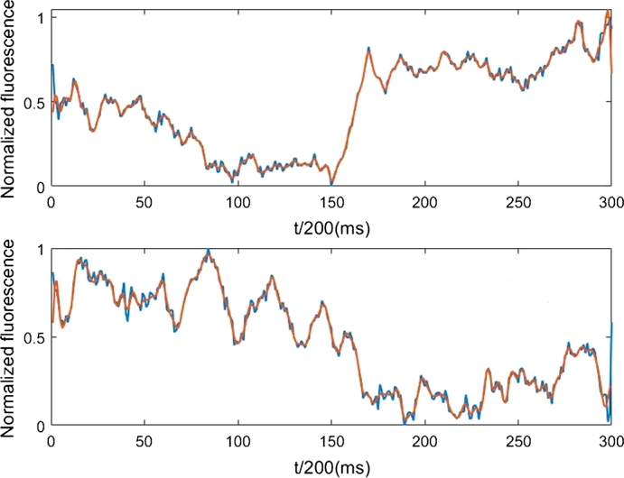
Above: A response to the olfactory stimulus given one time (in blue) and the same signal filtered (in red). Below: B response to the olfactory stimulus given one time (in blue) and the same signal filtered (in red).
Several sets of data (time series) have been collected using different type of stimula to activate the neurons and to all of them the Wiener-Granger method has been applied producing the same result, described in Section 4.
4. Study of neural signals
We start by applying the AR algorithm to the filtered neural signal B plotted in Fig. 1. The study described in the following was applied to all the collected neural signals, but for brevity in this paper just one case is reported with a single application of the odorant. Fig. 2 shows again the filtered B data from Fig. 1, together with the result of the AR(4) algorithm. The results of the AR(4) fits the data very well, with .
Figure 2.
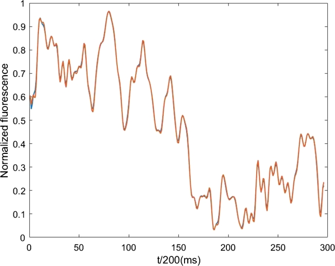
Signal from the B neuron (blue line) and from the AR(4) algorithm (red line).
We next apply the ARMA(4,) to reconstruct the B signal from itself and from the A data (Fig. 1). For this test we vary , the number of past bins of A that are used, from 0 to 50. Fig. 3 exhibits the RMS calculated from different ARMA(4,) models as a function of . For the RMS is as for the AR(4). If in addition to the four past values of the B function also past values of A are considered, the prediction improves with the increase of the number of these values. Next, only three values of B are considered. Fig. 4 shows the RMS of different ARMA(3,) for increasing values of . Also the RMS achieved by the ARMA(3,) models decreases with . However it always remains higher than the RMS of AR(4).
Figure 3.
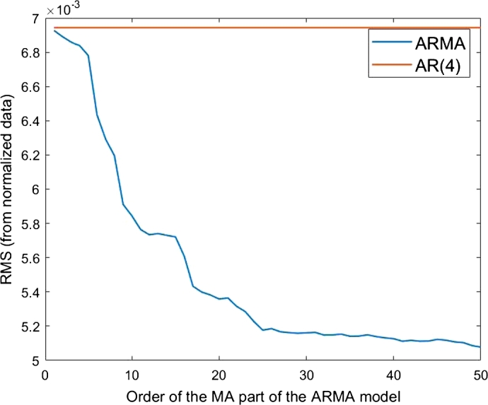
RMS of the ARMA(4,Q′) models as a function of Q′ (blue line). The RMS of the AR(4) model is shown as a red line.
Figure 4.
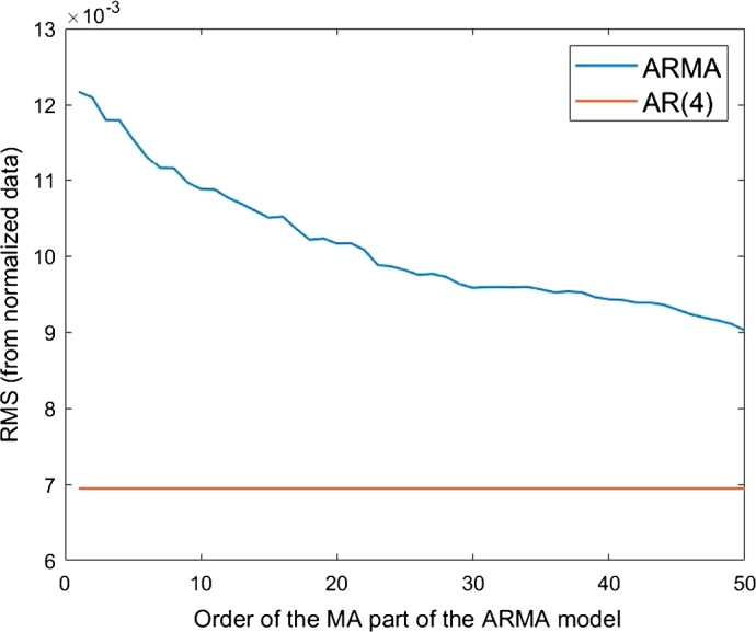
RMS of the ARMA(3,Q′) models as a function of Q′ (blue line). The RMS of the AR(4) model is shown as a red line.
One might argue that Figure 3, Figure 4 show a Granger causality between the neurons A and B because considering past values of A leads to a better description of B.
However, one could also say that the quality of a fit always increases with the number of parameters and also add that the agreement between the AR(4) prediction and data shown in Fig. 2 is already so good that there is hardly any room for a physics driven improvement: therefore the observed improvement might be only numerical.
To decide which interpretation is correct the test described in the following Section is applied.
4.1. Inverted A signal
According to Granger “The past and present may cause the future, but the future cannot cause the past” [2]. Therefore, if the results of the ARMA method shown in Figure 3, Figure 4 are evidence for Granger causality, they should not any more indicate Granger causality when applied to a time inverted A signal.
Fig. 5 shows the time inverted A signal on the bottom compared with the original one, on top, as already plotted in Fig. 1 (on top).
Figure 5.
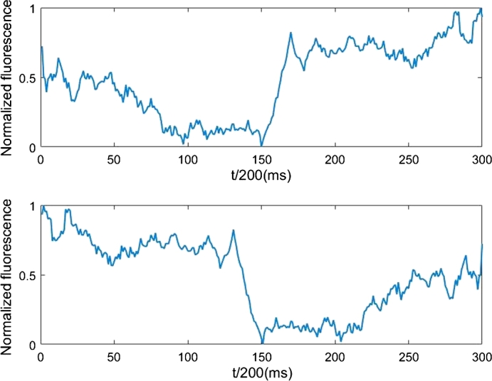
Top: the original A signal obtained with a single repetition of the olfactory stimulus which originated at the same time the B signal in Fig. 2. Bottom: the same A signal, but inverted.
The resulting ARMA(3,) and ARMA(4,) are shown in Figure 6, Figure 7 and display a similar behaviour to the ones in Figure 3, Figure 4.
Figure 6.
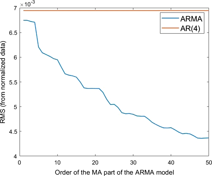
RMS of the AR(4) model (red line) and RMS of the ARMA(4,Q′) models as a function of Q′ (blue line). The inverted A signal in considered.
Figure 7.
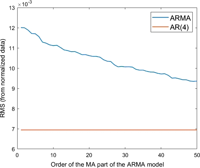
RMS of the AR(4) model (red line) and RMS of the ARMA(3,Q′) models as a function of Q′ (blue line). The inverted A signal in considered.
This means that the degrees of the RMS values of Figure 3, Figure 4 cannot be taken as an evidence of causality and that therefore the procedure proposed by Granger does not show any causality between A and B. However from past studies A is already known to be causal for B.
At this point a more fundamental study of the AR and ARMA algorithms is needed.
5. The differential calculus for the local reconstruction of the Fourier series
It is generally known that any function can be constructed from its Fourier components and that any point of a sine function can be calculated from two other points of the same function using the relation:
| (5) |
where and .
In a binned distribution it is possible to calculate the value of the sine function in a certain bin from the two previous bins by choosing ; for a given time interval Δt the bin width of a sinusoidal function is related to its frequency.
This means that if one considers different sinusoidal functions with same Δt but different frequency, for a given , there will be corresponding coefficients and (having fixed .
As a consequence, if the Fourier transform of a certain function is known, the value of the function at a certain time can be expressed using its values in previous times; in this case the bin width corresponds to the time step Δt. In the context of our study it has to be noted that this is true for any function that can be expressed as a Fourier series, regardless from the fact that this function has a physics meaning.
Alternatively for a differentiable function the value of the function in a certain bin can be calculated from the values in previous bins applying the differential calculus introduced by Newton: the value of a function f at a point , , can be approximated from its previous value by:
| (6) |
For a binned function this means:
| (7) |
with and . This approximation becomes more precise as the bin width decreases.
Equation (7) takes into account the first derivative. The approximation under certain conditions will increase in precision if we consider higher derivatives.
Taking for example the second derivative we obtain:
| (8) |
with , and .
While for the next order we have:
| (9) |
with , , and .
The Newtonian interpolation will become more precise with a decreasing bin width, while the parameters of Equation (5) are analytically precise.
This means, for instance, that for the reconstruction of a sinusoidal function the M and N parameters from Equation (5) will converge towards 2 and −1 from Equation (7) with decreasing bin widths. It has to be remembered that the bin width depends on both time and frequency: if, for a given frequency , this convergence has reached a certain precision, then for all the frequencies smaller than the agreement will further improve; therefore for frequencies smaller than the same coefficient can always be used in the Newton approximation. One would then expect that in a Fourier series, the lower the frequency of the examined component, the better the Newton approximation will result in a good prediction for the function. The high frequencies sinusoidal components of the series should instead be better approximated with the AR method. We note that in most physics data high frequencies are associated with noise, while the low frequencies components contain the physics feature of the system under observation. This is studied quantitatively in the next Section.
5.1. AR method
In Equations (7) to (9) the parameters are obtained from a general geometric argument and for large bin width are not optimized. The AR algorithm instead will find the best possible values for these coefficients from a numerical fit. Therefore the values obtained from the AR algorithm should converge towards the Newton values found above for small bin widths.
In a first step we apply the AR(2) algorithm to a binned sine function. That is, we calculate the expected value of the function in a bin from the values in the two preceding bins, using the AR(2) algorithm. Table 1 shows the and coefficients found with the AR(2) method for three different bin widths.
Table 1.
Values of the AR(2) a1 and a2 coefficients for decreasing bin widths.
| Bin width (in rad) | a1 | a2 |
|---|---|---|
| 1.9021 | −1.000 | |
| 1.9890 | −1.000 | |
| 1.9961 | −1.000 |
As expected, the fitted values for and converge towards the values 2 and -1 found in Equation (7) with a decreasing bin widths.
Table 2 shows the agreement of a sine function with its Newtonian extrapolation (from Equations (7), (8) and (9)) in terms of RMS (with binning ).
Table 2.
RMS obtained with the use of an increasing number of previous values of the sine function multiplied by the Newton coefficients.
| Number of past values | Coefficients value | RMS |
|---|---|---|
| 2 | 2, −1 | 0.0699 |
| 3 | 3, −3, 1 | 0.0214 |
| 4 | 4, −6, 4, −1 | 0.0069 |
In the next step the neural B function is studied (see Fig. 1).
Table 3 shows the coefficients obtained from the AR(2), AR(3) and AR(4) models and the RMS values of their fit, for different filter's values. For comparison also the RMS is shown if the Newton coefficients of Table 2 are applied instead of the ones coming from the AR fit.
Table 3.
Coefficients from the different AR models and RMS calculated with the AR and Newton methods for different number of preceding values. B signals without filtering, with cutting frequency at 0.16 and with cutting frequency at 0.008 are considered.
| Non filtered B signal | |||
|---|---|---|---|
| AR coefficients | RMS | RMS | |
| 2 | 0.9438, 0.0485 | 0.0608 | 0.0828 |
| 3 | 0.9413, 0.0117, 0.0393 | 0.0609 | 0.1384 |
| 4 | 0.9393, 0.0077, 0.0858, −0.0398 | 0.0608 | 0.2522 |
|
| |||
| B signal with cutting frequency at 0.16 | |||
|---|---|---|---|
| AR coefficients | RMS | RMS | |
| 2 | 1.6838, −0.6890 | 0.0212 | 0.0238 |
| 3 | 2.3226, −2.0298, 0.7060 | 0.0122 | 0.0197 |
| 4 | 2.9904, −3.7965, 2.5387, −0.7342 | 0.0069 | 0.0185 |
|
| |||
| B signal with cutting frequency at 0.008 | |||
|---|---|---|---|
| AR coefficients | RMS | RMS | |
| 2 | 1.9668, −0.9679 | 0.0025 | 0.0026 |
| 3 | 2.9419, −2.9106, 0.9687 | 3.9511 ⋅ 10−4 | 5.7784 ⋅ 10−4 |
| 4 | 3.8981, −5.7480, 3.8001, −0.9502 | 9.7855 ⋅ 10−5 | 1.6561 ⋅ 10−4 |
Table 3 shows in its third section (cutting frequency at 0.008) that for a function without noise, or with very little noise, the coefficients found with the AR method are very similar to those obtained with the Newton method listed in Table 2. The difference between them is of the order of 5%. This last section also shows that the RMS values obtained from the AR method are only slightly better than the ones obtained from the Newton method, for the B function with little noise. Increasing the amount of noise (as in the other sections of Table 3) increases the RMS values and the coefficients found from the AR method become very much different from the Newton ones. The first section, corresponding to the non filtered B signal, also shows that in the presence of a relevant noise the AR model always gives a value close to one for the coefficient, while the other coefficients turn out to be close to zero. This means that the reconstructed value in any point is essentially identical to the preceding value. In addition two coefficients are enough to make a prediction: adding more doesn't improve the RMS.
All in all the Newton and AR methods lead to the same results in the case of a function with low level of noise. This means that the AR method essentially consists of the prediction of the function from its preceding value and the derivatives in preceding points, regardless of the physics meaning of the function; in other words the coefficients found by the AR mechanism should be always the same for all kind of physics experiment, in the absence of high frequencies in the Fourier spectrum.
In the presence of noise the coefficients obtained from the AR model become clearly more effective than the simple application of the Newton constant from Table 2: the AR algorithm has an higher capability to fit the noise.
The fact that the Newton method is able to reconstruct all kinds of differentiable functions with the same coefficients means that it does not contain “information” about the physics content of the function.
When instead an AR algorithm is performed, the resulting decrease of the RMS values compared to the Newton ones is not due to the fact that the AR fit takes the physics signal into account better, but rather the noise.
With respect to the following discussion we note that for example the AR mechanism should reconstruct the time inverse of a function as well as the function itself.
5.2. ARMA method
The first graph showed by Fig. 8 depicts the RMS obtained from the AR(P) algorithm as a function of P for the same data used in Table 3: the B signal without filter, filtered with cutting frequency at 0.16 and with cutting frequency at 0.008 respectively. The second graph shows the RMS obtained from the AR(P) algorithm as a function of P for a simulated noise function with the same three filters.
Figure 8.
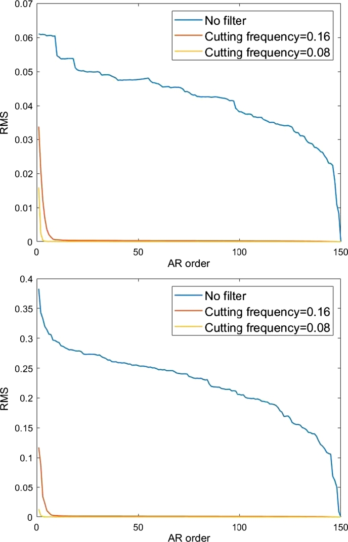
Top: RMS values for increasing order P of the AR method applied to the B function unfiltered and with a medium and a strong filter applied. Bottom: RMS values for the AR(P) reconstruction of a simulated noise function as a function of the P order, for different filtering.
We see that for the RMS reaches the 0 value. This is because corresponds to only 150 bins left in the time series to be fitted: we then have a system with 150 unknowns and 150 equations. We see in Fig. 8 in more detail what we already showed with Table 3: when high frequencies are removed from a function, the differential mechanism allows one to effectively reconstruct the function with fewer points. In the presence of high frequencies the convergence of the optimization program is much slower. As showed by Fig. 8 these considerations are true for any kind of function.
We next apply the MA algorithm, from Equation (2), on the neural time series A in order to calculate B: that is we predict B from A without making use of the data in the series B as described by Equation (2). The result of this is depicted in the first graph of Fig. 9, where we show the RMS obtained from the MA(Q) algorithm as a function of Q for different filtering applied to reconstruct the B signal from the A one. The second graph shows the results of the same procedure applied after substituting the A signal with a simulated noise signal.
Figure 9.
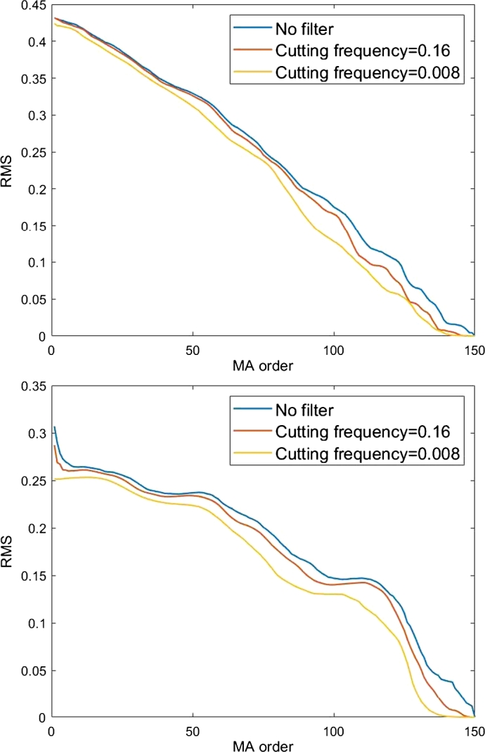
Top: RMS values for increasing order of the MA model applied to reconstruct B starting from A, for different filtering on both signals. Bottom: RMS values for increasing order of the MA model applied to reconstruct B starting from a simulated noise function, for different filtering on both signals.
We see again that the RMS becomes 0 at for the same reasons discussed before. Now for the reconstruction of the B Fourier series the knowledge of the Fourier series of the other signal is not useful; therefore filtering the function does not impact the reconstruction. The comparison between the two graphs in Fig. 9 shows that the same kind of behaviour is to be expected for all kind of functions regardless from their shape or physics meaning, and for all combination of functions.
One can as well reconstruct the B signal from the time inverted A signal: this confirms what already obtained in Section 4.1.
Instead of reconstructing B from itself (as done in the first graph of Fig. 8) or B from A (as done in the first graph of Fig. 9) we can also mix both the procedures: doing this, results in what is referred to as ARMA method. In the first graph of Fig. 10 we show the RMS obtained from the ARMA(4,) algorithms applied to B and A with different filtering, as a function of . The second graph shows the RMS obtained from the ARMA(4,) algorithms applied to B and a simulated noise function as a function of , with the same three different filters.
Figure 10.
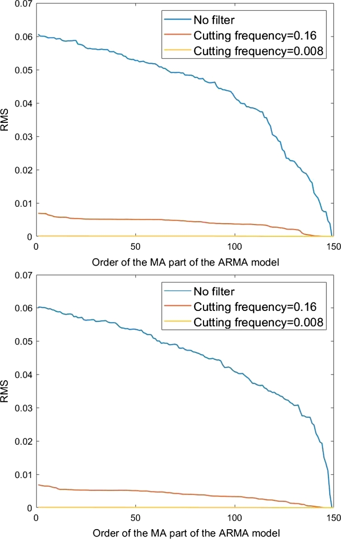
Top: RMS values for increasing Q′ of the ARMA(4,Q′) models for different filtering on the A and B signals. Bottom: RMS values for increasing Q′ of the ARMA(4,Q′) models for different filtering on the simulated noise function and B signals.
The comparison between these two graphs shows that the ARMA algorithm is not sensitive to the physics meaning of the “predicted” or “predicting” functions. However, the development of the RMS with very much depends on the presence of high frequencies contributions.
6. Interpretations
Granger may have believed that Equation (3) is expressing causality because an event at a time interval k is calculated from events in previous time intervals . One has to consider however that the coefficients are obtained from a fit from the entire data-set prior to applying this algorithm; therefore the algorithm does not express causality in the usual significance of the expression.
One might argue that Granger uses the term “causality” in a different way compared to the usual significance, and one might correspondingly define “causality” as what is expressed by the Granger formalism and to “predict” as whatever is done by Equation (3). However, this assumption leads to inconsistencies. First, we showed that with Granger Equation (3) any time series can be “predicted” from any other one. Differences in the RMS distribution for different time series are due to the properties of the Fourier transform only. Secondly, we found that Equation (3) “predicts” a time series A from a time series B equally well when the time series B is time inverted. Which means that Equation (3) predicts the past from the future as well as the future from the past. This constitutes an internal contradiction with the Granger's statement already cited in Section 5: “the past and present may cause the future, but the future cannot cause the past'. The Wiener-Granger algorithm seems not to have the power to describe causality in a meaningful way.
7. Conclusion
The ARMA algorithm which was used by Granger to determine the causality between time series is not able to give any evidence of such a causality. In spite of this, many studies have been performed under the assumption that the ARMA algorithm which was used by Granger to determine the causality between time series is able to give evidence of such a causality.
The Granger algorithm concerns fundamental questions about information, information processing and the meaning of messages, as can be seen in all the papers published on the Granger causality and in particular in Granger's original paper, where he used the word “information” forty times. This suggests that a more profound investigation of these fundamental notations is needed from a physics point of view.
Author contribution statement
Greta Grassmann: Conceived and designed the analysis; Analyzed and interpreted the data; Contributed analysis tools or data; Wrote the paper.
Funding Statement
This research did not receive any specific grant from funding agencies in the public, commercial, or not-for-profit sectors.
Competing Interest Statement
The authors declare no conflict of interest
Additional Information
Supplementary content related to this article has been published online at https://doi.org/10.1016/j.heliyon.2020.e05208.
Footnotes
Supplementary content related to this article has been published online at https://doi.org/10.1016/j.heliyon.2020.e05208.
Supplementary material
The following Supplementary material is associated with this article:
Appendix A provides details on how the series of neuronal activities have been collected, together with a brief description of the neurons' behaviour.
References
- 1.Granger Clive W.J. Investigating causal relations by econometrics models and cross-spectral methods. Econometrica. 1969;37 [Google Scholar]
- 2.Granger Clive W.J. Testing for causality. A personal viewpoint. J. Econ. Dyn. Control. 1980;2 [Google Scholar]
- 3.Seth Anil K., Barrett Adam B., Barnett Lionel. Granger causality analysis in neuroscience and neuroimaging. J. Comput. Neurosci. 2015 doi: 10.1523/JNEUROSCI.4399-14.2015. [DOI] [PMC free article] [PubMed] [Google Scholar]
- 4.Kim S., Putrino D., Ghosh S., Brown E.N. A Granger causality measure for point process models of ensemble neural spiking activity. PLoS Comput. Biol. 2011;7 doi: 10.1371/journal.pcbi.1001110. [DOI] [PMC free article] [PubMed] [Google Scholar]
- 5.Kispersky T., Gutierrez G.J., Marder E. Functional connectivity in a rhythmic inhibitory circuit using Granger causality. Neural Syst. Circuits. 2011;1(9) doi: 10.1186/2042-1001-1-9. [DOI] [PMC free article] [PubMed] [Google Scholar]
- 6.Gerhard F. Successful reconstruction of a physiological circuit with known connectivity from spiking activity alone. PLoS Comput. Biol. 2013;9 doi: 10.1371/journal.pcbi.1003138. [DOI] [PMC free article] [PubMed] [Google Scholar]
- 7.Eichler M. A graphical approach for evaluating effective connectivity in neural systems. Philos. Trans. R. Soc. Lond. B, Biol. Sci. 2005;360:953–967. doi: 10.1098/rstb.2005.1641. [DOI] [PMC free article] [PubMed] [Google Scholar]
- 8.Stokesa Patrick A., Purdon Patrick L. A study of problems encountered in Granger causality analysis from a neuroscience perspective. Proc. Natl. Acad. Sci. USA. 2017 doi: 10.1073/pnas.1704663114. [DOI] [PMC free article] [PubMed] [Google Scholar]
- 9.Chen Junya, Feng Jianfeng, Lu Wenlian. A Wiener causality defined by divergence. Neural Process. Lett. 2020:1–22. [Google Scholar]
- 10.Ashrafulla Syed. Canonical Granger causality applied to functional brain data. Biomed. Imag. IEEE Int. Symp. 2012;9:1751–1754. [Google Scholar]
- 11.Beebee Helen. Oxford University Press; Oxford: 2009. The Oxford Handbook of Causation. [Google Scholar]
- 12.Bressler Steven L., Seth Anil K. Wiener-Granger causality: a well established methodology. NeuroImage. 2011;58(2):323–329. doi: 10.1016/j.neuroimage.2010.02.059. [DOI] [PubMed] [Google Scholar]
- 13.Geweke John. Comparing alternative tests of causality in temporal systems: analytic results and experimental evidence. J. Econom. 1983;21(2):161–194. [Google Scholar]
- 14.Conway Roger K. The impossibility of causality testing. Agricultur. Econ. Res. 1984;36(3):1–19. [Google Scholar]
- 15.Maziarz Mariusz. A review of the Granger-causality fallacy. J. Philos. Econ.: Reflections on Economic and Social Issues. 2015 [Google Scholar]
- 16.Chalsani Sreekanth H., Chronis Nikos, Tsunozaki Makato, Gray Jesse M., Ramot Daniel, Goodman Miriam B., Bargmann Cornelia I. Nature Publishing Group; 2007. Dissecting a Circuit for Olfactory Behaviour in Caenorhabditis Elegans. [DOI] [PubMed] [Google Scholar]
- 17.Grassmann G. Università degli Studi di Trieste; Settembre 2019. Causalità di Wiener-Granger applicata a serie temporali estratte da C. elegans. (Tesi di Laurea in Fisica). [Google Scholar]
- 18.White J.G., Southgate E., Thomson J.N., Brenner S. The structure of the nervous system of the nematode Caenorhabditis elegans. Philos. Trans. R. Soc. Lond. B, Biol. Sci. 1986;314(1165) doi: 10.1098/rstb.1986.0056. [DOI] [PubMed] [Google Scholar]
Associated Data
This section collects any data citations, data availability statements, or supplementary materials included in this article.
Supplementary Materials
Appendix A provides details on how the series of neuronal activities have been collected, together with a brief description of the neurons' behaviour.


