Super-STORM: Molecular Modeling to Achieve Single-molecule Localization with STORM Microscopy

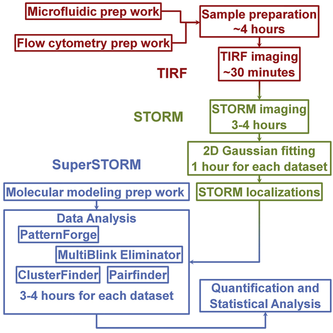
Summary

This protocol introduces the SuperSTORM technique, combining stochastic optical reconstruction microscopy (STORM) and molecular modeling. SuperSTORM is optimized for acquiring and processing STORM images of neutrophil integrins but can be used for any cell-surface molecule with known structure and antibody-binding site(s). SuperSTORM identifies molecular cut-offs for eliminating multiple blinks of STORM imaging, determines colocalization, identifies clusters, and reveals molecular orientations and distributions. This protocol extends STORM imaging to cells in microfluidic systems. Improved resolution is achieved by using biomolecule-inherent parameters.

For complete information on the generation and use of this protocol, please refer to the paper by Fan et al. (2019).

Graphical Abstract

Highlights

• •SuperSTORM combines STORM and molecular modeling to improve resolution
• •SuperSTORM identifies molecular cut-offs to find individual protein molecules
• •SuperSTORM reveals clusters, molecular orientations and distributions
• •SuperSTORM works with any STORM microscope

This protocol introduces the SuperSTORM technique, combining stochastic optical reconstruction microscopy (STORM) and molecular modeling. SuperSTORM is optimized for acquiring and processing STORM images of neutrophil integrins but can be used for any cell-surface molecule with known structure and antibody-binding site(s). SuperSTORM identifies molecular cut-offs for eliminating multiple blinks of STORM imaging, determines colocalization, identifies clusters, and reveals molecular orientations or distributions. This protocol extends STORM imaging to cells in microfluidic systems. Improved resolution is achieved by using biomolecule-inherent parameters.

BEFORE YOU BEGIN

Molecular Modeling Prep Work

• 1.Find crystal structures of your molecules in PDB; here, we used Integrin α_Xβ₂ ectodomain, PDB 3K6S (Figure 1)
• 2.Model in proper orientation and conformation (for example, top view, by CCP4MG)
• 3.If you are using antibodies, make F(ab) or scFv fragments (Pierce Fab Preparation Kit).

Note: This makes your probe smaller (more precise location) and eliminates possible interactions with Fc receptors on your cells.

• 4.Find epitopes
• 5.Model antibody (F(ab) or scFv) to epitopes
• 6.Label your antibody F(ab)s

Note: The distance estimation using site-directed fluorochrome labeling will be more accurate than random.

• a.There are site-directed methods for antibody or F(ab) labeling. In this case, you should know the fluorochrome labeling site, which will guide your further estimation. If you use N-hydroxysuccinimide ester-reactive fluorochrome labeling, and you know the sequence of the F(ab), you will know which residues were labeled.
• b.If you know the sequence of the antibody or F(ab) you used, the labeling sites can be predicted (primary amines, –NH₂) when using N-hydroxysuccinimide ester-reactive fluorochrome labeling.
• c.The antibody or F(ab) labeling should be considered random in your distance estimation if the antibody or F(ab) is labeled by N-hydroxysuccinimide ester-reactive fluorochrome labeling and if you don’t know the sequence of the antibody or F(ab).
• d.Suggested fluorochromes: Several fluorochromes have been tested for STORM imaging. In our experience (Fan et al., 2019), Dylight 550 and 650 are useful. AlexaFluor 647 (Huang et al., 2008), AlexaFluor 555 (Huang et al., 2008), and Atto-488 (Johnson et al., 2016) are also compatible with STORM imaging.
• 7.Modeling:
• a.If the antibody or F(ab) was labeled randomly, model fluorochrome positions in the same F(ab) (recommended 100,000 pairs of random spatial positions, get 100,000 values of distance).

Note: The size of an F(ab) from the top-view is known, e.g., 4 nm × 7 nm. Randomly generate two dots (x = RANDBETWEEN (0,400)/100, y = RANDBETWEEN (0,700)/100, in Excel). The distance of the two dots can be calculated as ((x₁-x₂)²+(y₁-y₂)²)^0.5.

• b.If site-directed, the distance between fluorochromes in the same F(ab) is known based on the structure.
• c.Model distance distribution of antibody signals bound to adjacent molecules (recommended 8 orientations, 8 directions of adjacency, 1,000 simulations for each condition for a total of 64,000 simulations, PatternForge).

Note: PatternForge is a PowerPoint/Excel based half-manual method (Figure 2, Supplemental Dataset 1). Relative locations of the two Fabs are determined in PowerPoint (Figure 2). The values of distance and orientations can be measured in PowerPoint (Positions and rotations of your objects). These values were used in the Excel spreadsheet for the random simulations (Supplemental Dataset 1)

Figure 1.

Integrin α_Xβ₂ Ectodomain

PDB 3K6S (https://www.rcsb.org/structure/3k6s). α_X and β₂ chains are labeled as dark and light blue, respectively.

Figure 2.

PatternForge

Sixty-four ways that two bent-high affinity β2 integrin molecules may be oriented (eight directions, in rows, and eight orientations, in columns). The simulation of each condition is included in the Supplemental Dataset 1.

• 8.Superimpose the distributions from step 7 to find the cut-off for eliminating multiple blinks from the same F(ab). Example is shown in Figure 3.
• 9.Eliminate multiple blinks from same F(ab) by using the merging function of ThunderSTORM (MultiBlink Eliminator), which is an open-source plugin in FIJI-ImageJ (Ovesný et al., 2014). The remaining blinks represent your F(ab) molecules.
• 10.Identify the molecular cut-off for the clusters at 99% (distance that covers 99% of all distances as determined in step 7c). Note that this cut-off will depend on the size of your molecule and the orientation and position of the F(ab) or scFv.
• 11.ClusterFinder: Find multiple-blinks-eliminated events within clusters by Imaris plugin software (calculating spot-to-spot closest distance). Events with a distance lower than the cut-off from step 10 are considered to be in a cluster.
• 12.If you have more than one F(ab), label the second one with a different fluorochrome and repeat steps 7-11 for the next antibody
• 13.Finding pairs: If you label your molecule with more than one Fab, you will want to know whether the signal comes from the same or adjacent molecules.
• 14.Determine the distance distribution between two antibodies or Fabs (labeled by different fluorochromes) when bound to the SAME molecule (100,000 random simulations, PatternForge)
• 15.Determine the distance distribution between two antibodies or Fabs (labeled by different fluorochromes) when bound to ADJACENT molecules (recommended 8 orientations, 8 directions of adjacency, 1000 random simulations for each for a total of 64,000 simulations, PatternForge)
• 16.Superimpose the distributions from 14 and 15 to determine the molecular cut-off for pairs, where the two distributions cross over. You will need this in the data analysis.

Note: A cut-off below the effective resolution produces unreliable data.

• 17.Find pairs by the custom algorithm (Pairfinder, Github)

Note: Pairfinder is an algorithm in MATLAB. In the algorithm, import the x and y location of the two channels and give a value of cut-off (Step 16). It will provide a list of pairs (x and y location of each channel).

• 18.
  Molecular orientations: to learn your molecular orientations, get the distance distribution of your molecules in the experimental data with the Imaris plugin software (calculating spot-to-spot closest distances).

  • a.
    Procedures: Open Imaris – Plugin “Image Processing” –
  • b.
    “Create Spots From File” to generate “Spots” in Imaris from your datasheet –
  • c.
    select the “Spots” of your data –
  • d.
    In the “Tools” tab, select “Spots to Spots Closest Distance” – “Spots Statistics” – “Center” –
  • e.
    After calculation, select “Statistics” tab – “Detailed” and export the data of “DistMin.”
• 19.
  Compare the distance distribution from the experimental data to the following distributions:

  • a.
    Random (Distribution from 8 orientations, all 64 conditions)
  • b.
    Face-to-face (Distribution from face-to-face conditions)
  • c.
    Parallel (Distribution from parallel conditions)
  • d.
    Back-to-back (Distribution from back-to-back conditions)
  • e.
    Use the Kolmogorov-Smirnov test to determine whether two distributions are different from each other. Using the p value may be too sensitive when comparing the distribution of experimental data to a simulated distribution. The D value, which represents the maximum distance between the cumulative distribution functions, is a better parameter to assess the fit. After comparing with the experimental data, consider the simulated distribution with the smallest D value a match.

Figure 3.

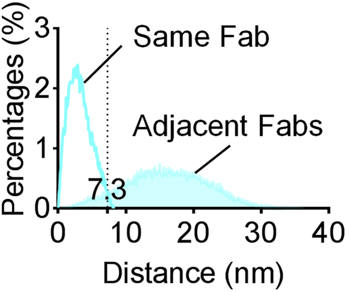
Molecular Cut-Off

Distance distributions of localizations emanating from the same mAb24 Fab (open) or mAb24 Fabs bound to adjacent integrin molecules (filled), based on simulations of 64,000 randomly oriented integrin molecules. Adopted from Figure 3F in Fan et al., 2019.

Microfluidic Prep Work (Optional)

• 20.Construct a microfluidic flow chamber that meets your needs (volume, shear stress, number of channels). A polydimethylsiloxane (PDMS) chip with a #1.5 glass coverslip is recommended.
• 21.Calibrate your microfluidic device by adjusting input and output pressures, calculating and measuring flow rates.
• 22.Calibrate your activation and fixation times based on cell transit at the desired shear stress. Mix the stimulus or fixing buffer with FITC and record your cell behavior (e.g., arrest) and the fluorescence of FITC. This determines the time at which the cell will arrest after the FITC appears for the stimulus or fixing buffer, respectively. If the fixing time is shorter than the stimulation time, then the difference (e.g., 12 s in Fan et al., 2019) will be used in the sample preparation: add the fixing buffer 12 s after adding the stimulus. If the fixing time is longer than the stimulation time, more optimization is needed (lower concentration of stimulus or higher concentration of fixing buffer).

Flow Cytometry Prep Work

• 23.
  Assess the purification and viability of the isolated or cultured cells. Assess the purity by the cell-specific markers, such as CD66b⁺Siglec-8^- for human neutrophils; assess the viability by staining, for example with Ghost Dyes™.

  • a.
    Wash isolated neutrophils with PBS twice and resuspended them in PBS at a concentration around 10⁷ cells per mL;
  • b.
    Stain cells with Ghost Dye™ Red 710 (1:1000) for 30 min on ice;
  • c.
    Wash cells with PBS plus 2% FBS and 1 mM EDTA twice and resuspend them in this buffer;
  • d.
    Add human Fc-blocker into the cell suspension (1:100);
  • e.
    Stain cells with anti-CD66b-FITC (1 μg·mL⁻¹) and anti-Siglec-8-PE (1 μg·mL⁻¹) for minutes on ice;
  • f.
    Wash cells with PBS twice and assessed by flow cytometry;
  • g.
    The purity of human neutrophils (CD66b⁺Siglec-8^-) is ∼97% (Figure 4A);
  • h.
    The viability of isolated neutrophils (Ghost Dye™ Red 710 negative) is ∼99% (Figure 4B).
• 24.
  Determine the site density of your epitopes on your cells, using calibration beads (Quantum Simply Cellular, Bangs Laboratories). You will need to know the number of molecules per μm² of surface area.

  • a.
    There are beads with five graded antibody binding capacities (ABC; 0, 14601, 72536, 204074, and 363264);
  • b.
    Stain beads with the same antibody you used for cell staining, such as FITC-Rat anti-mouse IgG1 (5 μg·mL⁻¹ for beads with 0, 14601, and 72536 ABC; 10 μg/mL for beads with 204074 ABC; 15 μg/mL for beads with 363264 ABC) for 10 min at 22-24°C;
  • c.
    Wash beads twice with PBS and access the fluorescence intensity by flow cytometry. The correlations of ABC and median fluorescence intensity (MFI) is shown in Figure 4C (ABC = MFI × 94.5);
  • d.
    Add human Fc-blocker into the cell suspension (1:100);
  • e.
    Stain cells with the antibody of the molecule you interested;
  • f.
    For example, isolated neutrophils (2 × 10⁶ mL⁻¹) were stained with KIM127 (mouse anti-human IgG1, 10 μg/mL) for 5 min at 22-24°C;
  • g.
    Stimulate cells with 200 ng·mL⁻¹ IL-8 for 30 s at 22-24°C and directly fixed cells with 1% PFA on ice for 10 min;
  • h.
    Wash cells twice with PBS plus 2% FBS and 1 mM EDTA twice and resuspend them in this buffer;
  • i.
    Stain cells with FITC-Rat anti-mouse IgG1 antibody (10 μg/mL) for 10 min at 22-24°C;
  • j.
    Wash cells twice with PBS and access the fluorescence intensity by flow cytometry. Use the equation above in step c to calculate the number of KIM127 epitopes on a cell.
• 25.Determine the maximum duration of the experiment during which the cells would still be alive and not activated for your assay (within 6 hours for human neutrophils in RPMI-1640 plus 2% HSA at 22-24°C)

CRITICAL: Make sure your cells are alive and not activated, using appropriate markers (CD11b and L-selectin for neutrophils).

• a.Stimulate isolated neutrophils with 1 μM fMLP or vehicle control for 10 min at 22-24°C and directly fixed cells with 1% PFA on ice for 10 min.
• b.Wash cells twice with PBS plus 2% FBS and 1 mM EDTA twice and resuspend them in this buffer.
• c.Add human Fc-blocker into the cell suspension (1:100).
• d.Stain cells with anti-CD11b-FITC or anti-L-selectin-FITC (10 μg·mL⁻¹ each) for 15 min at 22-24°C. Isotype controls were used to assess the background fluorescence;
• e.Wash cells twice with PBS and access the fluorescence intensity by flow cytometry.
• f.For neutrophils that were not activated, the increase of CD11b surface expression (Figure 4D) and L-selectin shedding (Figure 4E) should be observed.
• 26.Make sure the cells can be activated and inhibited as planned
• 27.Find a suitable cell surface marker. We find abundant GPI-linked proteins to work best, e.g., CD16 for human neutrophils.
• 28.Find the appropriate concentration of antibodies/F(ab)s to label molecules of interest. The concentration is determined by the staining saturation assay using flow cytometry.

Figure 4.

Flow Cytometry Prep Work

(A) Dot plot showing the purity of human neutrophil isolation assessed by staining of CD66b and Siglec-8.

(B) Dot plot showing the viability of isolated human neutrophils assessed by staining of Ghost Dye™. EtOH killed cells were served as a positive control (left plot).

(C) Linear correlations of the antibody binding capacity (ABC) and the median fluorescence intensity (MFI) of calibration beads.

(D) Histogram showing the expression of CD11b on neutrophil surface before (gray) and after (green) fMLP stimulation. Isotype control is shown as the open black curve.

(E) Histogram showing the expression of L-selectin on neutrophil surface before (gray) and after (red) fMLP stimulation. Isotype control is shown as the open black curve. In this example, viability was 99% (B), CD11b upregulation by fMLP was > 3-fold (D) and L-selectin was expressed by all resting neutrophils (E). This indicates healthy neutrophils.

KEY RESOURCES TABLE

REAGENT or RESOURCE	SOURCE	IDENTIFIER
Antibodies
Anti-human β2 integrin (clone mAb24) Fab	Biolegend	Customized
Anti-human β2 integrin (clone KIM127)	Lymphocyte Culture Center at the University of Virginia	Customized
Anti-human CD11b (FITC, clone ICRF44)	Biolegend	Cat# 301330
Anti-human L-selectin (PE, DREG-56)	Biolegend	Cat# 304806
Anti-human CD66b (FITC, clone G10F5)	Biolegend	Cat# 305104
Anti-human Siglec-8 (PE, clone 7C9)	Biolegend	Cat# 347104
anti-human CD16 (AF488, clone 3G8)	Biolegend	Cat# 302019
anti-human CD16 (AF647, clone 3G8)	Biolegend	Cat# 302020
Anti-human β2 integrin (AF488, clone mAb24)	Biolegend	Cat# 363404
anti-human CD14 (BV421, clone M5E2)	Biolegend	Cat# 325627
Rat anti-mouse IgG1 (FITC, clone RMG1-1)	Biolegend	Cat# 406606
Biological Samples
Human blood from healthy donors	LJI	N/A
Chemicals, Peptides, and Recombinant Proteins
Recombinant human P-selectin-Fc	R&D Systems	Cat# 137-PS-050
Recombinant human ICAM-1 -Fc	R&D Systems	Cat# 720-IC-050
Recombinant human IL-8	R&D Systems	Cat# 208-IL-010
Recombinant human CCL2	Biolegend	Cat# 571402
Recombinant human TNF-α	Biolegend	Cat# 570102
Casein blocking buffer	Thermo Fisher	Cat# 37528
Fluorescein (FITC)	Thermo Fisher	Cat# 46425
CellTracker Orange CMRA	Thermo Fisher	Cat# C34551
CellTrace Violet	Thermo Fisher	Cat# C34557
CellMask DeepRed	Thermo Fisher	Cat# C10046
Ghost Dye™ Red 710	Tonbo Biosciences	Cat# 13-0871-T500
Polymorphprep	Cosmo Bio	Cat# AXS-1114683
Ficoll-Paque Plus	GE Healthcare	Cat# 17144003
Human Serum Albumin (HSA)	Gemini	Cat# 800-120
Paraformaldehyde	Thermo Fisher	Cat# 28906
Glutaraldehyde	Sigma-Aldrich	Cat# G5882-10X1ML
Mercaptoethanolamine	Sigma-Aldrich	Cat# M9768-5G
Glucose Oxidase from Aspergillus niger	Sigma-Aldrich	Cat# 49180
Catalase from bovine liver	Sigma-Aldrich	Cat# C9322
Nanodiamond (100 nm Carboxylated Red FND,~3ppm NV,1 mg/mLin DI water,10 ml)	Adamasnano	Cat# NDNV100nmHi10ml
Critical Commercial Assays
Pierce™ Fab Preparation Kit	Thermo Fisher	Cat# 44985
DyLight™ 550 Microscale Antibody Labeling Kit	Thermo Fisher	Cat# 84531
DyLight™ 650 Microscale Antibody Labeling Kit	Thermo Fisher	Cat# 84536
Quantum Simply Cellular anti-Mouse	Bangs Laboratories	Cat# 810
EasySep™ Human Monocyte Enrichment Kit without CD16 Depletion	StemCell	Cat# 19058
Endothelial SingleQuots Kit	Lonza	Cat# CC-4176
Deposited Data
Raw data of E-H+ αXβ2 integrin crystal structure	Protein Data Bank	PDB: 4NEH
Raw data of Fab crystal structure	Protein Data Bank	PDB: 3HI6
Raw data of E-H- αXβ2 integrin crystal structure	Protein Data Bank	PDB: 3K6S
Raw data of H+ αIIBβ3 integrin crystal structure	Protein Data Bank	PDB: 3FCU
Electron microscopy image of E+H+ β2 integrin	Chen et al., 2012	N/A
Electron microscopy images of E- and E+ β2 integrin	Chen et al., 2010	N/A
Experimental Models: Cell Lines
Hybridoma of KIM127	ATCC	Cat# CRL-2838
HUVEC	ATCC	Cat# CRL-1730
Primary human neutrophils	This paper	N/A
Primary human monocytes	This paper	N/A
Software and Algorithms
FIJI-ImageJ2	Rueden et al., 2017	imagej.net/ImageJ2
Imaris 9.0	Bitplane	https://imaris.oxinst.com/
Nikon STORM software	Nikon	N/A
Thunder STORM	Ovesny et al., 2014	github.com/zitmen/thunderstorm
CCP4MG	McNicholas et al., 2011	www.ccp4.ac.uk/MG
Prism 7	GraphPad	graphpad.com
MATLAB	MathWorks	www.mathworks.com/products/matlab.html
Pairfinder	Custom Algorithm on Github	https://github.com/saramcardle/Image-Analysis-Scripts/blob/master/Super%20Resolution/MutualNearestNeighbors.m
NanoHills	Custom Algorithm on Github	https://github.com/saramcardle/Image-Analysis-Scripts/blob/master/Super%20Resolution/TirfZforStorm_commented.m
PowerPoint (for PatternForge)	Microsoft Office	https://www.office.com/
Excel (for PatternForge)	Microsoft Office	https://www.office.com/
Other
Roswell Park Memorial Institute (RPMI) medium 1640 without phenol red	Thermo Fisher	Cat# 11835055
phosphate-buffered saline (PBS) without Ca2+ and Mg2+	Thermo Fisher	Cat# 10010049
Phenol Red Free Endothelial Cell Growth Basal Medium	Lonza	Cat# CC-3129
μ-Slide VI 0.5 Glass Bottom chambers	ibidi	Cat#

MATERIALS AND EQUIPMENT

Equipment

• •Microfluidic device

The assembly of the microfluidic devices used in this study and the coating of coverslips with recombinant human P-selectin-Fc and ICAM-1-Fc has been described previously (Fan et al., 2016, Sundd et al., 2012, Sundd et al., 2011, Sundd et al., 2010, Sun et al., 2020). Briefly, cleaned coverslips were coated with P-selectin-Fc (2 μg ml-1) and ICAM-1-Fc (10 μg ml-1) for 2 hours and then blocked for 1 hour with casein (1%) at 22-24°C. After coating, coverslips were sealed to polydimethylsiloxane (PDMS) chips by magnetic clamps to create flow chamber channels ∼29 μm high and ∼300 μm across. By modulating the pressure between the inlet well and the outlet reservoir, 6 dyn cm⁻² wall shear stress was applied in all experiments.

• •STORM microscope

Images were captured using a 100 × 1.49 NA Apo total internal reflection fluorescence (TIRF) objective with TIRF (80° incident angle) illumination on a Nikon Ti super-resolution microscope. Images were collected on an ANDOR IXON3 Ultra DU897 EMCCD camera using the multicolor sequential mode setting in the NIS-Elements AR software (Nikon Instruments Inc., NY). Power of the 488, 561, and 647-nm lasers was adjusted to 50% to enable collection of between 100 and 300 blinks per 256 × 256 pixel camera frame in the center of the field at appropriate threshold settings for each channel. The collection was set to 20,000 frames, yielding 1–2 million molecules.

• •Workstation for image processing

Due to the large raw data files and heavy workload in image processing, a workstation installed with proper software listed above is required.

Hardwares of the workstation used in (Fan et al., 2019):

CPU: Intel - Xeon E5-1650 V4 3.6 GHz 6-Core Processor

CPU Cooler: Phanteks - PH-TC12DX 68.5 CFM CPU Cooler

Motherboard: Gigabyte - GA-X99-Designare EX ATX LGA2011-3

Memory: 2 × Kingston - ValueRAM 32 GB (1 × 32 GB) Registered DDR4-2133

Storage: SanDisk - X400 1 TB M.2-2280 Solid State Drive

Hitachi - Ultrastar He8 8 TB 3.5” 7200RPM Internal Hard Drive

Video Card: MSI - GeForce GTX 1080 8 GB Video Card

Recipes in Fan et al., 2019

• •Protein coating: human P-selectin-Fc (2 μg·ml^-1) and ICAM-1-Fc (10 μg·ml^-1) for 2 hours and then blocked for 1 hour with casein (1%) at 22-24°C.
• •Medium for the neutrophil suspension: RPMI-1640 without phenol red plus 2% HSA.
• •Antibody/F(ab) concentration in staining: mAb24-F(ab)-DL550 (5 μg·ml^-1), KIM127-F(ab)-DL650 (5 μg·ml^-1)
• •Stimulation and fixation: IL-8 (10 ng·ml⁻¹) for 12 s and then 8% PFA for 5 min.
• •STORM buffer: 50 mM Tris pH 8.0, 10 mM NaCl, 10% Glucose, 0.1 M Mercaptoethanolamine (Cysteamine Sigma-Aldrich), 56 U/mL Glucose Oxidase (from Aspergillus niger, Sigma-Aldrich), and 340 U/mL Catalase (from bovine liver, Sigma-Aldrich)

Alternates

• •Other microscopes are compatible with single-molecule localization imaging (different vendors or in-house).
• •Other demonstrated formula of STORM buffer.
• •Other demonstrated dyes compatible with STORM, for example Alexa Fluor 647, Alexa Fluor 555, Atto 488.
• •0.01% Glutaraldehyde may be introduced into the fixation buffer to stabilize the membrane morphology.
• •Flow chamber: Another flow chamber may be used in the experiments, such as vacuum-sealed PDMS microfluidic chip on a μ-Slide 2 Well Glass Bottom Chamber (ibidi).
• •Fiducial markers: Besides nanodiamonds, fluorescent microspheres (diameter ≤ 200 nm, multiple fluorochrome-labeled) can be used as fiducial markers. The advantage of microspheres is that they are cheaper and might be brighter than nanodiamonds in some channels, such as a 647-nm laser. However, microspheres will be photobleached during the image acquisition and are less accurate than nanodiamonds due to uneven labeling of different fluorochromes.

STEP-BY-STEP METHOD DETAILS

Assemble the Microfluidic Device

Timing: ∼3 h

• 1.Coat the coverslip of the microfluidic device with the biological molecules of interest, for example, coat 2 μg·mL⁻¹ human P-selectin-Fc and 10 μg·mL⁻¹ human ICAM-1-Fc for 2 hours at 22-24°C on a 25 mm diameter round coverslip as in Fan et al., 2019.
• 2.Coat nanodiamonds, 100 nm diameter fiducial markers together with proteins in step 1. 1:500 dilution from the original concentration.
• 3.Block with 1% casein for 30 min at 22-24°C.
• 4.Wash twice with PBS.
• 5.Assemble the flow chamber under buffer to avoid buffer-air interfaces (Figure 5)
• 6.Prepare Petri dishes (50 mm diameter) with a hole in the bottom (15 mm diameter).

Figure 5.

Microfluidic Set Up

The PDMS microfluidic chip is sealed on top of a 1.5# 25mm-diameter coverglass by magnetic clamp to form nine parallel microfluidic channels with a height of 29 μm and a width of 300 μm. The coverglass is coated with adhesion molecules (2 μg·mL⁻¹ P-selectin, 10 μg·mL⁻¹ ICAM-1) to support leukocyte rolling and adhesion. The shear stress is generated by modulating the water-level between inlet and outlet reserves.

Cell Isolation and Labeling

Timing: ∼1–1.5 hours

Note: This can be performed during the 2-hour coating of coverslips.

• 7.Isolate cells from culture, blood or tissue. Polymorphoprep was used for the isolation of human neutrophils from blood in Fan et al., 2019. Wash with PBS without Ca²⁺ and Mg²⁺ twice.
• 8.Resuspend the cells in RPMI-1640 without phenol red plus 2% HSA.

Note: Culture media may vary for different cell types.

• 9.Add cell surface label by membrane dyes (a, b) or evenly distributed surface molecules (c)
• a.CellMask Green, CellMask Orange, CellMask Deep Red
• b.DiO, DiI, DiD
• c.A fluorescently labeled antibody/F(ab) to an abundant GPI-anchored cell surface antigen, such as CD16 on neutrophils as in Fan et al., 2019. Cells were stained with AF488-anti-CD16 antibody (1 μg·mL⁻¹) for 10 min at 22-24°C, washed twice with PBS, and resuspended in RPMI-1640 without phenol red plus 2% HSA.

Note: In most cases, an abundant GPI-anchored cell surface antigen is the best to label cell surface due to minimum bleed through. However, it may be hard to find a homogenously distributed molecule for the cell type of interest. Membrane dyes in a and b might be too bright and may interfere with STORM imaging, especially that short-wavelength dyes may bleed through to long-wavelength channels. Using a lower concentration of the membrane dyes may be helpful. Using a long-wavelength dye (CellMask Deep Red or DiD) may avoid the bleed through but will occupy the best STORM imaging channel (AlexaFluor 647 or Dylight 650).

• d.Wash with PBS without Ca²⁺ and Mg²⁺ twice after staining. Then resuspend the cells in RPMI-1640 without phenol red plus 2% HSA.
• 10.Label the molecules of interest: Integrin extension (E⁺) and high affinity (H⁺) were reported by F(ab) fragments of KIM127 and mAb24, respectively. Cells (5 × 10⁶ mL⁻¹) were incubated with KIM127 and mAb24 F(ab) fragments (5 μg mL⁻¹ each) at 22-24°C for 3 min and perfused into the microfluidic chamber without F(ab) separation.
• a.Label the molecules before the fixation to avoid any epitope loss by the fixation.
• b.There is an increase of integrin activation epitopes upon IL-8 stimulation during neutrophil rolling and arrest. There may also be a change in expression (number of molecules). This may require additional controls, like a F(ab) that binds the molecule of interest independent of its conformation.
• c.For molecules that do not change their level of expression, label the molecules of interest in the appropriate condition. Wash cells before perfusing into the flow chamber to reduce the background of unspecific binding on the coverslip.

PAUSE POINT: Potential pause point up to 2 hours

Sample Preparation

Timing: ∼1 hour

• 11.Add cells (5 × 10⁶ ml^-1) to the reservoir of the microfluidic device (cell concentration may vary depending on the cell type and microfluidic device)
• 12.Apply pressure to start the flow.
• 13.Add activator (for example, IL-8 for human neutrophils, 10 ng·mL⁻¹, 12 s in Fan et al., 2019) The process of neutrophil rolling and arrest is shown in Figure 6.
• 14.Add fixation buffer (for example, add the same volume of 16% PFA to the reservoir, final concentration 8% in Fan et al., 2019) for 5 min, keep perfusing while observing cells using a bright-field microscope.
• 15.Wash for 5 min using the same buffer in which the cells are suspended, without any air bubbles.

CRITICAL: This avoids generating an interface that could detach the cells.

Optional: Add your labeled antibodies/F(ab)s to the perfusate for 5 minutes to saturate the labeling.

Optional: Wash for 5 min with the same buffer in which the cells are suspended.

• 16.Disassemble microfluidic device

CRITICAL: Glue the coverslip into the hole of the Petri dish with Super Glue (Gorilla) to avoid any leakage or movement/drifting, and cells face up.

• 17.Fill the Petri dish with 2 mL PBS.

PAUSE POINT: Up to 24 hours

Figure 6.

Neutrophil Rolling and Arrest

Representative bright-field images showing the process of neutrophil rolling and arrest on the substrate of P-selectin/ICAM-1/IL-8 under a shear stress of 6 dyn·cm^-2. Scale bar is 10 μm.

STORM Imaging

Timing: ∼3–4 hours

• 18.Transfer the sample to the microscope, for example Nikon Ti super-resolution inverted microscope, equipped with a 100x 1.49 NA Plan Apo TIRF oil objective and an ANDOR IXON3 Ultra DU897 EMCCD camera (The EM gain we used was 300 in the Nikon system), field of view 82 × 82 μm², should contain about 3-7 cells, TIRF mode at 80 degrees incident angle.

CRITICAL: Replace PBS with 2 mL freshly made STORM buffer in the Petri dish.

• 19.Acquire one TIRF image (Figure 7A) at each wavelength (low laser power (typical 0.5%–2%) and 200 ms exposure time, typically one for the surface marker, 2 for molecules of interests, and an optional one to distinguish different cell subtypes)

Note: laser power and exposure time may vary due to different microscopy setup. A setting giving a signal-to-noise ratio larger than 5 should be applied.

• 20.Acquire raw images from the exact same field of view (high laser power, typically 50%, and 10ms exposure time), typically 20,000 frames per channel, in the two channels (back and forth) imaging the fluorochromes that were used to label the molecules of interest

Note: laser power and exposure time may vary due to different microscopy setup. You want to use high power to put all the fluorochromes in the dark state so they can “blink” well. You want to have a very short exposure time so two “blinks” within the diffraction limit (∼200-300 nm) will not be “on” in the same frame. In our study (Fan et al., 2019), the power of the 488, 561, and 647-nm lasers was adjusted to 50% to enable collection of between 100 and 300 blinks per 256 × 256-pixel camera frame in the center of the field at appropriate threshold settings for each channel. The number of frames acquired may vary from 10,000 to 60,000. It is advisable to test different numbers of frames and determine where the image stops improving. There are several quantitative metrics for determining the number of acquisition frames (Culley et al., 2018, Endesfelder et al., 2014).

• 21.During step 20, apply an automatic drifting correction (implemented in the Nikon N-STORM software) using fiducial markers (nanodiamonds in Assemble the microfluidic device step 2)

Note: Most vendors have their own drifting correction software implemented.

• 22.Determine the localization of molecules using 2D Gaussian fitting (implemented in the Nikon software)

Note: The effective lateral resolution needs to be smaller than the size of the molecule studied.

• 23.Generate and store data sheets of all STORM localizations, which can be shown as a pointillism map (Figure 7B).
• 24.Register the TIRF image from step 19 with the STORM positions
• a.Take advantage of the fiducial markers
• b.Generate a STORM image using ThunderSTORM: “Visualization” – “Visualization options” – “Normalized Gaussian” – “Lateral Uncertainty” = λ/2/N.A. (λ is the excitation wavelength) – “OK”
• c.Register the TIRF image with the STORM image using bUnwrapJ Plugins in FIJI-ImageJ.
• 25.Convert TIRF signal to distance map using NanoHills (Github)

PAUSE POINT: (time unlimited)

Figure 7.

TRIF and STORM Images of Integrin Activation

Representative images of KIM127 (magenta) and mAb24 (cyan) on the footprint of an IL-8 triggered arrest neutrophil on the substrate of P-selectin/ICAM-1. (A) TIRF image, adopted from Figure 1A in Fan et al., 2019. (B) Pointillism map of the localization data from the STORM acquisition, adopted from Figure 2A in Fan et al., 2019. Scale bar is 1 μm.

Analysis of STORM Images

Timing: (∼3–4 hours for each dataset)

• 26.Sample data is available in the Supplemental Dataset 2.
• 27.Eliminate multiple blinks from each F(ab) or scFv using the molecular cut-off in Molecular modeling prep work steps 8-9
• 28.Identify clusters using the molecular cut-off from Molecular modeling prep work step 11
• 29.Identify pairs using the molecular cut-off from Molecular modeling prep work step 17
• 30.Calculate the distance distributions for each of the conformations your antibodies/F(ab)s report using Imaris Plugin software (in Fan et al., 2019, we had 3 visible conformations: E⁺H⁻, E⁻H⁺, E⁺H⁺. E⁻H⁻ was invisible because we used no conformation-independent antibody)
• 31.
  Compare measured distributions, for example to

  • a.
    Random
  • b.
    Face-to-face
  • c.
    Parallel
  • d.
    Back-to-back

Expected Outcomes

Sample data is available in the Supplemental Dataset 2.

Number of molecules after eliminating multiple blinks: This is an estimation of the number of molecules expressed on the cell footprint within TIRF range (about 150 nm vertical distance from coverslip). This number can be used for a quantitative comparison of the molecular/conformation expression between control and experimental groups.

Number and proportion of molecules in clusters: This is a parameter that shows the clustering of molecules of interest.

Number, size, and ellipticity of clusters: This shows the morphology parameters of clusters.

Number of colocalization pairs: This reflects the colocalization of molecules and can be expressed as a percentage of all molecules detected.

Student’s t test, Mann-Whitney test, and one-way ANOVA test are suitable for the above data. Which test to use depends on the number of samples per group and the number of groups being compared to each other.

Distance distribution of molecules: This is useful to investigate the spatial orientation of molecules after comparing with simulated data of different patterns (random, face-to-face, parallel, and back-to-back). This distribution can be compared using the Kolmogorov-Smirnov test. The median distance of the distribution is another parameter to compare, using a t test or one-way ANOVA test based on the number of groups.

Limitations

For molecules without structure information or antibodies without mapped epitopes, SuperSTORM cannot be used. The limits of current STORM technique dictate that no more than three channels can be used for super-resolution images. Different dyes behave differently. Dye switching experiments can control for this. STORM only works on fixed cells.

Troubleshooting

Problem

Impropriate coating concentration of fiducial markers in STORM imaging.

Potential Solution

Try different coating concentration to get a good density of fiducial markers during imaging. Normally, one field-of-view should have 10-20 fiducial markers.

Problem

Fiducial markers are too bright or dim during the acquisition.

Potential Solution

Try different microscopy setting to optimize the brightness of your fiducial markers. They should not be too bright to out-range the limits of the camera. They should not be too dim to identify (Signal-to-noise ratio should be more than 10). Please change to a different kind of fiducial marker if it does not meet your requirement.

Problem

Drifting during the STORM acquisition.

Potential Solution

You can acquire 1,000 test frames to assess the drifting of your image using fiducial markers. Drifting should be less than 50 nm during the 1,000 frames. This data is also useful to test your software of drifting correction. If drifting is too severe, please try using the air table, changing the location of your microscope, or avoiding temperature changes of the sample to resolve the problem.

Problem

Fluorochromes do not blink.

Potential Solution

Coat the coverslip with fluorochromes or fluorochrome-labeled antibodies and try different microscopy settings (mainly the laser power) to get blinking. Blinking means you should see one excitation spot, and then it should be dark immediately in the next frame. Choose a condition where the blinks are not too dense – less than 300 spots per field-of-view. Change the microscope setting or use a different fluorochrome to get blinks.

Problem

Fluorochromes are too bright or dim.

Potential Solution

Try different settings to optimize the brightness. The brightness of one blink should be more than 1,000 photon counts. The brightness Gaussian of all your blinks should have a peak around 3,000-4,000 photon counts. Change the microscope setting or use a different fluorochrome to adjust the brightness.

Problem

Fluorochromes are photobleach too fast.

Potential Solution

The laser setting should be chosen to ensure that the number of blinks does no decrease over the number of frames acquired (minimal photobleaching). Use more amount of the STORM buffer to get less photobleaching.

Problem

Background noise is too high.

Potential Solution

Dirt on the coverslip may fluoresce. Thus, coverslip cleaning is very important for STORM imaging. Use 1 M NaOH solution to clean the coverslip (22-24°C, 20 min).

Problem

Difficulty in disassembling the flow chamber and gluing it to the Petri dish

Potential Solution

This step is the transition step from sample preparation to STORM imaging. To keep the STORM stable, avoid any residual flow in the chamber during imaging. Thus, the flow chamber needs to be disassembled.

During the disassembling, it is critical to have some medium remaining in the inlet well, so the medium will flow onto the coverslip. The coverslip should never become dry (the buffer-air interface immediately denatures proteins). Disassemble the flow chamber while immersed in PBS to prevent the coverslip from sticking onto the PDMS chip.

After disassembling, vacuum out most liquid on your coverslip beside the sample region. To glue the coverslip onto a Petri dish with a hole, the area of gluing needs to be dry.

Use Super Glue, not tape or nail polish to glue the coverslip onto the Petri dish. Only super glue is strong enough to avoid excessive drifting during imaging.

Problem

No blinking during imaging.

Potential Solution

The possible reason causing “no blinking” is that you don’t have enough STORM buffer on your sample. Make sure the volume of STORM buffer on your sample is more than 0.5 mL.

Some fluorochromes will not blink, such as FITC, PE, most fluorescent proteins.

You may also want to check your staining by TIRF imaging or flow cytometry.

Supplemental Information

Supplemental Dataset 1

The Spreadsheet for the Random Simulation and Calculation of the PatternForge

Supplemental Dataset 2

Sample Data of STORM Acquisition Showing the Localizations of mAb24-AF647 Blinks on the Footprint of an Arrested Neutrophil

References

- Chen X., Xie C., Nishida N., Li Z., Walz T., Springer T.A. Requirement of open headpiece conformation for activation of leukocyte integrin alphaXbeta2. Proceedings of the National Academy of Sciences of the United States of America. 2010;107:14727–14732. doi: 10.1073/pnas.1008663107. [DOI] [PMC free article] [PubMed] [Google Scholar]
- Chen X., Yu Y., Mi L.Z., Walz T., Springer T.A. Molecular basis for complement recognition by integrin alphaXbeta2. Proceedings of the National Academy of Sciences of the United States of America. 2012;109:4586–4591. doi: 10.1073/pnas.1202051109. [DOI] [PMC free article] [PubMed] [Google Scholar]
- Culley S., Albrecht D., Jacobs C., Pereira P.M., Leterrier C., Mercer J., Henriques R. Quantitative mapping and minimization of super-resolution optical imaging artifacts. Nat. Methods. 2018;15:263–266. doi: 10.1038/nmeth.4605. [DOI] [PMC free article] [PubMed] [Google Scholar]
- Endesfelder U., Malkusch S., Fricke F., Heilemann M. A simple method to estimate the average localization precision of a single-molecule localization microscopy experiment. Histochem. Cell Biol. 2014;141:629–638. doi: 10.1007/s00418-014-1192-3. [DOI] [PubMed] [Google Scholar]
- Fan Z., McArdle S., Marki A., Mikulski Z., Gutierrez E., Engelhardt B., Deutsch U., Ginsberg M., Groisman A., Ley K. Neutrophil recruitment limited by high-affinity bent β2 integrin binding ligand in cis. Nat. Commun. 2016;7:12658. doi: 10.1038/ncomms12658. [DOI] [PMC free article] [PubMed] [Google Scholar]
- Fan Z., Kiosses W.B., Sun H., Orecchioni M., Ghosheh Y., Zajonc D.M., Arnaout M.A., Gutierrez E., Groisman A., Ginsberg M.H. High-Affinity Bent beta2-Integrin Molecules in Arresting Neutrophils Face Each Other through Binding to ICAMs In cis. Cell Rep. 2019;26:119–130.e115. doi: 10.1016/j.celrep.2018.12.038. [DOI] [PMC free article] [PubMed] [Google Scholar]
- Huang B., Jones S.A., Brandenburg B., Zhuang X. Whole-cell 3D STORM reveals interactions between cellular structures with nanometer-scale resolution. Nat. Methods. 2008;5:1047–1052. doi: 10.1038/nmeth.1274. [DOI] [PMC free article] [PubMed] [Google Scholar]
- Johnson J.L., He J., Ramadass M., Pestonjamasp K., Kiosses W.B., Zhang J., Catz S.D. Munc13-4 Is a Rab11-binding protein that regulates Rab11-positive vesicle trafficking and docking at the plasma membrane. J. Biol. Chem. 2016;291:3423–3438. doi: 10.1074/jbc.M115.705871. [DOI] [PMC free article] [PubMed] [Google Scholar]
- McNicholas S., Potterton E., Wilson K.S., Noble M.E. Presenting your structures: the CCP4mg molecular-graphics software. Acta crystallographica Section D, Biological crystallography. 2011;67:386–394. doi: 10.1107/S0907444911007281. [DOI] [PMC free article] [PubMed] [Google Scholar]
- Ovesný M., Křížek P., Borkovec J., Svindrych Z., Hagen G.M. ThunderSTORM: a comprehensive ImageJ plug-in for PALM and STORM data analysis and super-resolution imaging. Bioinformatics. 2014;30:2389–2390. doi: 10.1093/bioinformatics/btu202. [DOI] [PMC free article] [PubMed] [Google Scholar]
- Rueden C.T., Schindelin J., Hiner M.C., DeZonia B.E., Walter A.E., Arena E.T., Eliceiri K.W. ImageJ2: ImageJ for the next generation of scientific image data. BMC bioinformatics. 2017;18:529. doi: 10.1186/s12859-017-1934-z. [DOI] [PMC free article] [PubMed] [Google Scholar]
- Sun H., Fan Z., Gingras A.R., Lopez-Ramirez M.A., Ginsberg M.H., Ley K. Frontline Science: A flexible kink in the transmembrane domain impairs beta2 integrin extension and cell arrest from rolling. Journal of leukocyte biology. 2020;107:175–183. doi: 10.1002/JLB.1HI0219-073RR. [DOI] [PMC free article] [PubMed] [Google Scholar]
- Sundd P., Gutierrez E., Pospieszalska M.K., Zhang H., Groisman A., Ley K. Quantitative dynamic footprinting microscopy reveals mechanisms of neutrophil rolling. Nat. Methods. 2010;7:821–824. doi: 10.1038/nmeth.1508. [DOI] [PMC free article] [PubMed] [Google Scholar]
- Sundd P., Gutierrez E., Petrich B.G., Ginsberg M.H., Groisman A., Ley K. Live cell imaging of paxillin in rolling neutrophils by dual-color quantitative dynamic footprinting. Microcirculation. 2011;18:361–372. doi: 10.1111/j.1549-8719.2011.00090.x. [DOI] [PMC free article] [PubMed] [Google Scholar]
- Sundd P., Gutierrez E., Koltsova E.K., Kuwano Y., Fukuda S., Pospieszalska M.K., Groisman A., Ley K. ‘Slings’ enable neutrophil rolling at high shear. Nature. 2012;488:399–403. doi: 10.1038/nature11248. [DOI] [PMC free article] [PubMed] [Google Scholar]
Associated Data
This section collects any data citations, data availability statements, or supplementary materials included in this article.
Supplementary Materials