COVID-19 spread and inter-county travel: Daily evidence from the U.S.

Abstract

Daily data at the U.S. county level suggest that coronavirus disease 2019 (COVID-19) cases and deaths are lower in counties where a higher share of people have stayed in the same county (or travelled less to other counties). This observation is tested formally by using a difference-in-difference design controlling for county-fixed effects and time-fixed effects, where weekly changes in COVID-19 cases or deaths are regressed on weekly changes in the share of people who have stayed in the same county during the previous 14 days. A counterfactual analysis based on the formal estimation results suggests that staying in the same county has the potential of reducing total weekly COVID-19 cases and deaths in the U.S. as much as by 139,503 and by 23,445, respectively.

Highlights

• •COVID-19 cases and deaths get lower with less inter-county travel within the U.S.
• •Restricting inter-county travel can reduce COVID-19 cases as much as by 139,503.
• •Restricting inter-county travel can reduce COVID-19 deaths as much as by 23,445.

1. Introduction

As of September 2nd, 2020, the number of people who have lost their lives in the U.S. due to the coronavirus disease 2019 (COVID-19) has reached 181,129, whereas the number of cases has reached 5,909,266.1 Since COVID-19 spreads mainly through person-to-person contact (e.g., see Chan et al. (2020)), different layers of government in the U.S. reacted to this development by implementing travel restrictions, both internationally and domestically, which is similar to other countries or other time periods (e.g., see Bajardi et al. (2011), Wang and Taylor (2016)), Charu et al. (2017) or Fang et al. (2020)). However, these restrictions do not cover the U.S. in a nationwide way, since the federal government has left such policy decisions to local governments.2

Based on this background, this paper investigates whether inter-county travel within the U.S. has any implications for COVID-19 cases or deaths. This is achieved by using U.S. daily data at the county level covering the period between January 21th, 2020 and September 2nd, 2020. Inter-county travel is measured by using data from smartphone devices. Descriptive statistics suggest that both COVID-19 cases and deaths are lower in counties where a higher share of people have stayed in the same county (or a fewer share of people have travelled across counties) during the previous 14 days.

Since descriptive statistics cannot control for any county-specific characteristics or time-specific changes that are common across counties, a formal investigation is achieved by using a difference-in-difference design, where county-fixed effects and time-fixed effects are controlled for. The estimation results suggest that if a person lives in a county where the average person has travelled less compared to the previous week, it is better for this person to stay in her county to reduce the possibility of catching COVID-19 as her county has lower COVID-19 cases or deaths due to other people in that county travelling less. However, if a person lives in a county where the average person has travelled more compared to the previous week, it is better for this person to travel as well (potentially to counties with lower COVID-19 cases) to reduce the possibility of catching COVID-19 as her county has higher COVID-19 cases or deaths due to other people in that county travelling more.

The estimation results are further used to answer the following hypothetical question based on a counterfactual analysis: What would happen to the number of COVID-19 cases and deaths in each county if all people would stay in the same county? The results suggest that staying in the same county has the potential of reducing total weekly COVID-19 cases and deaths in the U.S. as much as by 139,503 and by 23,445, respectively. At the county level, staying in the same county has the potential of reducing COVID-19 cases between 2 and 209 across counties, and it has the potential of reducing county-specific COVID-19 deaths up to 35. It is implied that staying in the same county (i.e., travelling less across counties) would help fighting against COVID-19. These results are consistent with other studies such as by Kraemer et al. (2020)) or Chinazzi et al. (2020) who have shown that the travel restrictions implemented in China have mitigated the spread of COVID-19.

The rest of the paper is organized as follows. The next section introduces the data set and methodology used. Section 3 depicts and discusses empirical results, while Section 4 concludes.

2. Data and estimation methodology

2.1. Data

Daily U.S. data on the cumulative number of COVID-19 cases and deaths at the county level have been obtained from New York Times.3 Daily data for inter-county travel have been borrowed from Chan et al. (2020).4 The latter data set has been constructed by using PlaceIQ data that describe smartphone devices “pinging” in a given geographic unit on a given day. Based on this information, once a certain number of smartphone devices are determined to be in a particular U.S. county on a particular day, the data set provides information on the share of these devices that have pinged in another U.S. county at least once during the previous 14 days.5 The combined sample covers the daily period between January 21th, 2020 and September 2nd, 2020 for 2018 U.S. counties.

Daily data for inter-county travel are used to obtain information on staying in the same county (or travelling less across counties) during the previous 14 days. Formally, given that there is a certain number of smartphone devices pinged in county c on time t, let's denote the share of these devices that have pinged in county i at least once during the previous 14 days with p _cit. Based on this notation, we consider the following definition for staying in the same county (or travelling less across counties) during the previous 14 days.

2.1.1. Staying in the same county (travelling less across counties)

The summation of shares of devices that have not pinged (even once) in any other county during the previous 14 days. In terms of the notation introduced, it is given by:

$$S_{c,t}=\sum _{i\ne c}\left(1-p_{\mathit{cit}}\right)$$ (1)

where S _c,t is the summation of shares of devices in county c that have not pinged in any other county during the previous 14 days. Since there are 2018 U.S. counties in our sample, S _c,t can take a value between 0 and 2017. As an example, 0.1 of an increase in S _c,t would correspond to 10% less people travelling to any other county during the previous 14 days. The extreme value of S _c,t=2017 would mean that out of the devices that are pinged in county c today, none of them have pinged in any other county during the previous 14 days; hence, all devices have been staying in county c during the previous 14 days in the case of S _c,t=2017. We will use this extreme case of S _c,t=2017 to have a counterfactual analysis below, where we will ask the following question: What would happen to the number of COVID-19 cases and deaths in each county if all devices would stay in the same county?

2.2. Descriptive statistics

For visual evidence, the treatment group is constructed as counties that have experienced a certain degree of an increase in S _c,t, whereas the control group is constructed as the other counties. To consider seasonality by construction, we work with weekly changes. In particular, first, for each county, we first calculate weekly changes in S _c,t as ΔS _c,t. Second, we find the maximum value of ΔS _c,t for county c during the sample period (i.e., max(ΔS _c,t|  c| )). If the maximum weekly change ΔS _{c, t} in county c is above a certain threshold (i.e., if max(ΔS _c,t|  c) > τ _c, where τ _c represents a county-specific threshold value), we consider county c as a same-county-stayer (or a less-travelling) county as a part of the treatment group; other counties are considered as the control group. For robustness, we consider four alternative threshold values for visual evidence. These threshold values are determined based on the distribution of max(ΔS _c,t|  c)’s across counties. Specifically, τ _c is defined as j ×  max (max(ΔS _c,t|  c)|  t), where j ∈ {0.2,0.4,0.6,0.8}. Therefore, we consider how much each county is close to those other counties experiencing a certain increase in their S _c,t measures.

2.2.1. Staying in the same county (or travelling less across counties)

When the number of COVID-19 cases in the U.S. are considered, the visual evidence based on travelling across counties (S _c,t measures) is provided in Fig. 1 and summarized in Table 1 . Using the threshold value of τ _c=0.9 to find the counties in the treatment group satisfying max(ΔS _c,t|  c) > τ _c results in having 354 less-travelling counties (treatment group) and 1664 more-travelling counties (control group). As is evident in Table 1 which shows the number of COVID-19 cases as of September 2nd, 2020 (i.e., the end of the sample period), less-travelling counties have about 2730 less cases on average across counties and 5,429,564 less total cases in the U.S. when the threshold value of τ _c=0.9 is used. As the threshold increases to τ _c=3.7, less-travelling counties have about 2734 less cases on average across counties and 5,907,258 less total cases in the U.S.

Fig. 1.

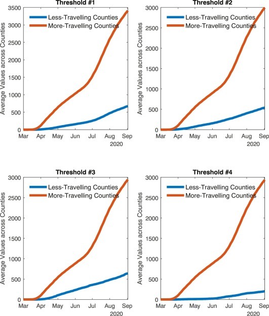
COVID-19 cases across U.S. counties.

Notes: Data are represented as weekly changes in daily variables. Less-travelling counties are defined as those where the maximum (during the sample period) weekly increase in the percentage of people who travel less is more than the threshold. Thresholds 1–4 represent τ_c = j ×  max (max(ΔS_c,t| c)| t) for j ∈ {0.2,0.4,0.6,0.8}.

Table 1.

COVID-19 cases as of September 2nd, 2020.

Treatment vs control groups	Threshold for less-travelling counties
	0.9	1.8	2.8	3.7
# of less-travelling counties	354	53	13	5
# of more-travelling counties	1,664	1,965	2,005	2,013
Average cases (treatment)	678	542	645	201
Average cases (control)	3,407	2,993	2,943	2,935
Treatment − control	−2,730	−2,451	−2,298	−2,734
Total cases (treatment)	239,851	28,721	8,380	1,004
Total cases (control)	5,669,415	5,880,545	5,900,886	5,908,262
Treatment − control	−5,429,564	−5,851,824	−5,892,506	−5,907,258

Notes: Less-travelling counties are defined as those where the maximum (during the sample period) weekly increase in the percentage of people who who stay in the same county is more than the threshold. Thresholds represent τ_c = j ×  max (max(ΔS_c,t| c)| t) for j ∈ {0.2,0.4,0.6,0.8}.

The corresponding historical patterns over time for the average COVID-19 cases (across counties) are given in Fig. 1. As is evident, independent of the threshold considered, less-travelling counties have experienced lower number of COVID-19 cases compared to more-travelling counties in the U.S., and the difference between these treatment and control groups gets higher for higher threshold values (as consistent with Table 1).

The results of a similar visual investigation for the number of COVID-19 deaths based on travelling across counties (S _{c, t} measures) are given in Fig. 2 and summarized in Table 2 . As is evident in Table 2 which shows the number of COVID-19 deaths as of September 2nd, 2020, less-travelling counties have about 15 less deaths on average across counties and 170,157 less total deaths in the U.S. when the threshold value of τ _c=0.9 is used. As the threshold increases to τ _c=3.7, less-travelling counties have about 88 less deaths on average across counties and 181,113 less total deaths in the U.S.

Fig. 2.

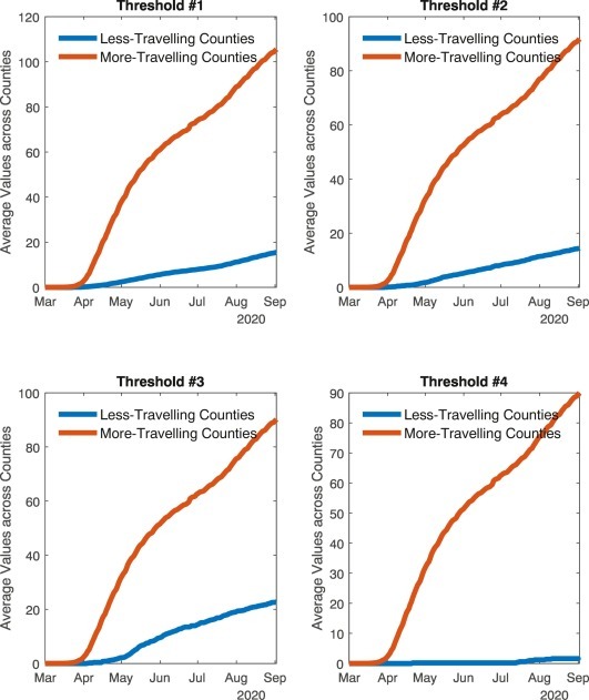
COVID-19 deaths across U.S. counties.

Notes: Data are represented as weekly changes in daily variables. Less-travelling counties are defined as those where the maximum (during the sample period) weekly increase in the percentage of people who travel less is more than the threshold. Thresholds 1–4 represent τ_c = j ×  max (max(ΔS_c,t| c)| t) for j ∈ {0.2,0.4,0.6,0.8}.

Table 2.

COVID-19 deaths as of September 2nd, 2020.

Treatment vs control groups	Threshold for less-travelling counties
	0.9	1.8	2.8	3.7
# of less-travelling counties	354	53	13	5
# of more-travelling counties	1,664	1,965	2,005	2,013
Average deaths (treatment)	15	15	23	2
Average deaths (control)	106	92	90	90
Treatment − control	−90	−77	−67	−88
Total deaths (treatment)	5,486	770	295	8
Total deaths (control)	175,643	180,359	180,834	181,121
Treatment − control	−170,157	−179,589	−180,539	−181,113

Notes: Less-travelling counties are defined as those where the maximum (during the sample period) weekly increase in the percentage of people who who stay in the same county is more than the threshold. Thresholds represent τ_c = j ×  max (max(ΔS_c,t| c)| t) for j ∈ {0.2,0.4,0.6,0.8}.

The corresponding historical patterns over time for the average COVID-19 deaths (across counties) are given in Fig. 2. As is evident, independent of the threshold considered, less-travelling counties have experienced lower number of COVID-19 deaths compared to more-travelling counties in the U.S., and the difference between the treatment and control groups gets higher for higher threshold values (as consistent with Table 2).

2.3. Formal investigation

The visual evidence provided so far does not control for any county-specific characteristics or time-specific changes that are common across counties. Moreover, the effects of staying in the same county (or travelling less across counties) may be asymmetric between counties depending on the sign of ΔS _c,t. In particular, positive (negative) values of ΔS _c,t represent counties that have travelled less (more) with respect to the previous week; hence, these county groups may be affected asymmetrically out of changes in ΔS _c,t. As an example, if a person lives in a county where people have travelled less with respect to the previous week (i.e., ΔS _c,t>0), that person may have a lower possibility of catching COVID-19, since lower number of people has the potential of having COVID-19 in that county due to travelling less. Similarly, if a person lives in a county where people have travelled more with respect to the previous week (i.e., ΔS _c,t<0), that person may have a higher possibility of catching COVID-19, since higher number of people has the potential of having COVID-19 in that county due to travelling more.

In order to capture these additional details, we achieve a formal investigation based on the following difference-in-difference specification:

$$\Delta D_{c,t}={\beta }_0+{\beta }_1^{+}\Delta S_{c,t}^{+}+{\beta }_2^{-}\Delta S_{c,t}^{-}+{\theta }_c+{\gamma }_t+{\epsilon }_{c,t}$$ (2)

where ΔD _c,t represents the weekly change in cumulative daily COVID-19 cases or deaths in U.S. county c at time t, ΔS _c,t ⁺ represents positive values of ΔS _c,t (i.e., counties that have travelled less with respect to the previous week) and ΔS _c,t ⁻ represents negative values of ΔS _c,t (i.e., counties that have travelled more with respect to the previous week). County fixed effects are represented by θ _c’s, and they capture county-c specific characteristics that are constant over time, such as the quality of the overall health system or the corresponding geographical location. Time fixed effects are represented by γ _t’s, and they capture day-specific developments that are common across U.S. counties such as declaration of national emergency (e.g., the one on March 13th, 2020 declared by the White House). Finally, ε _c,t represents residuals.

Using Eq. (2), we consider the following question: Do cumulative daily COVID-19 cases or deaths in same-county-stayer (i.e., less-travelling) counties change differently from those in other counties? This question is answered by the difference-in-difference specification in Eq. (2) as ΔS _c,t ⁺ or ΔS _c,t ⁻ measures correspond to continuous treatments. It is important to emphasize that this specification already considers a time delay (of up to 14 days) by construction due to the way that ΔS _{c, t} is measured that is necessary for the effects of inter-county travel to show up on COVID-19 cases or deaths.

2.4. Counterfactual analysis

Once Eq. (2) is estimated, we further use the corresponding results to ask the following hypothetical question as briefly described above.

2.4.1. Hypothetical question

What would happen to the number of COVID-19 cases and deaths in each county if all devices would stay in the same county? This question can be answered by comparing the latest situation of counties (at the end of the sample period) with the hypothetical case of S _c,H=2017. Formally, based on Eq. (2) that controls for county fixed effects and time fixed effects, since all devices staying in the same county would correspond to a positive value of ΔS _c,t, this can be achieved by using the following expression:

$$\Delta D_{c,H}={\beta }_1^{+}\Delta S_{c,H}={\widehat{\beta }}_1^{+}\left(S_{c,H}-S_{c,T}\right)={\widehat{\beta }}_1^{+}\left(2017-S_{c,T}\right)$$ (3)

where ΔD _c,H represents hypothetical weekly change in COVID-19 cases or deaths in county c, β ₁ ⁺ is the estimated coefficient in Eq. (2) for positive values of ΔS _c,t, ΔS _c,H is the hypothetical (positive) weekly change in S _c,t (since S _c,T<2017), and S _c,T is the latest value of S _c,t at time t = T (end of the sample period). The sum of ΔD _c,H across counties can further be used to obtain information on the U.S. level:

$$\Delta D_{\mathit{US},H}=\sum _c\Delta D_{c,H}$$ (4)

where ΔD _US,H represents hypothetical weekly change in COVID-19 cases or deaths in the U.S. if all devices would stay in the same county.

3. Empirical investigation

3.1. Estimation results

The results of estimating Eq. (2) are given in Table 3 , where the effects of ΔS _c,t on ΔD _c,t are distinguished between positive and negative values of ΔS _c,t. As is evident, given that more people stay in the same county compared to the previous week (i.e., ΔS _c,t>0), weekly changes in both COVID-19 cases and COVID-19 deaths react negatively to the weekly change in S _c,t, suggesting that both COVID-19 cases and COVID-19 deaths can be reduced by staying in the same county. The corresponding coefficient of β ₁ ⁺ suggests that 10% less people travelling to any other county would reduce weekly COVID-19 cases by about 2 and weekly COVID-19 deaths by about 0.3, on average across U.S. counties. It is implied that if a person lives in a county where the average person has travelled less compared to the previous week, it is better for this person to stay in her county to reduce the possibility of catching COVID-19 as her county has lower COVID-19 cases or deaths due to other people in that county travelling less. Therefore, if people in all counties would reduce inter-county travel, total number of COVID-19 cases and deaths can be reduced (as we analyze more during the counterfactual investigation, below).

Table 3.

Estimation results.

	Dependent variable: weekly changes in total
	Daily COVID-19 cases	Daily COVID-19 deaths
Weekly positive changes in	−20.82∗∗∗	−3.499∗∗∗
Same-county stayers	(5.437)	(0.402)
Weekly negative changes in	18.13∗∗	2.797∗∗∗
Same-county stayers	(6.086)	(0.450)
County fixed effects	Yes	Yes
Time fixed effects	Yes	Yes
Sample size	421,762	421,762
R−squared	0.405	0.277
Adjusted R−squared	0.402	0.273

Notes: ** and *** represent significance at the 1% and 0.1% levels.

Standard errors are in parentheses.

As is also evident in Table 3, given that more people travel across counties compared to the previous week (i.e., ΔS _c,t<0), weekly changes in both COVID-19 cases and COVID-19 deaths react positively to the weekly change in S _c,t. The corresponding coefficient of β ₁ ⁻ suggests that 10% less people travelling to any other county would increase weekly COVID-19 cases by about 2 and weekly COVID-19 deaths by about 0.3, on average across U.S. counties. It is implied that if a person lives in a county where the average person has travelled more compared to the previous week, it is better for this person to travel as well (potentially to counties with lower COVID-19 cases) to reduce the possibility of catching COVID-19 as her county has higher COVID-19 cases or deaths due to other people in that county travelling more.

3.2. Counterfactual investigation

What would happen to the number of COVID-19 cases and deaths in each county if all devices would stay in the same county? The answer to this hypothetical question is given in Table 4 , where ΔD _c,H measures across counties based on Eq. (3) as well as the aggregate-level result ΔD _US,H for the U.S. based on Eq. (4) are given.

Table 4.

Counterfactuals: all devices staying in the same county.

Estimates across counties:	Weekly changes in total
	Daily COVID-19 cases	Daily COVID-19 deaths
Average	−69	−12
Median	−67	−11
Minimum	−209	−35
Maximum	−2	0
Total (for the U.S.)	−139,503	−23,445

Notes: Counterfactuals are based on the estimated coefficients in Table 3.

As is evident, staying in the same county has the potential of reducing total weekly COVID-19 cases and deaths in the U.S. as much as by 139,503 and by 23,445, respectively. Staying in the same county has the potential of reducing COVID-19 cases between 2 and 209 across counties, and it has the potential of reducing county-specific COVID-19 deaths up to 35. It is implied that staying in the same county (i.e., travelling less across counties) would help fighting against COVID-19.

3.3. Discussion of results

This section discusses the empirical results by connecting them to the existing literature. Overall, the results based on the counterfactual investigation suggest that both COVID-19 cases and COVID-19 deaths can be reduced by travelling less across counties. This is consistent with other studies such as by Kraemer et al. (2020) or Chinazzi et al. (2020) who show that the travel restrictions implemented in China have mitigated the spread of COVID-19.

The results are also in line with studies such as by Linka et al. (2020) who show that an unconstrained mobility would have significantly accelerated the spreading of COVID-19 in Central Europe, Spain, and France. The results are consistent with studies such as by Browne et al. (2016) or Lau et al. (2020) as well, since they show how travel accelerates and amplifies the propagation of influence and a strong correlation between travellers versus the number of domestic and international COVID-19 cases, respectively.

Regarding policy suggestions, it is implied that restrictions on inter-county travel may help fighting against COVID-19 as the movement of people affects the number of infected people and the duration of the disease severely (e.g., see Denphedtnong et al. (2013)). Since individual behavior change is essential in terms of mitigating emerging infectious diseases as indicated in studies such as by Yan et al. (2018), policies supporting media publicity focused on how to guide people's behavior change may further help fighting against COVID-19.

4. Conclusion

This paper has investigated the effects of people staying in the same county (i.e., travelling less across counties) on the county-level COVID-19 cases or deaths in the U.S. during the daily period between January 21th, 2020 and September 2nd, 2020. Descriptive statistics suggest that both COVID-19 cases and deaths are lower in counties where a higher share of people have stayed in the same county (or travelled less to other counties).

Since descriptive statistics cannot control for any county-specific characteristics or time-specific changes that are common across counties, a formal investigation has been achieved by using a difference-in-difference design, where county-fixed effects and time-fixed effects have been controlled for. The corresponding results have suggested that if a person lives in a county where the average person has travelled less compared to the previous week, it is better for this person to stay in her county to reduce the possibility of catching COVID-19 as her county has lower COVID-19 cases or deaths due to other people in that county travelling less. However, if a person lives in a county where the average person has travelled more compared to the previous week, it is better for this person to travel as well (potentially to counties with lower COVID-19 cases) to reduce the possibility of catching COVID-19 as her county has higher COVID-19 cases or deaths due to other people in that county travelling more.

A counterfactual analysis based on the formal estimation results further suggests that staying in the same county has the potential of reducing total weekly COVID-19 cases and deaths in the U.S. as much as by 139,503 and by 23,445, respectively. At the county level, staying in the same county has the potential of reducing COVID-19 cases between 2 and 209 across counties, and it has the potential of reducing county-specific COVID-19 deaths up to 35. It is implied that staying in the same county (i.e., travelling less across counties) would help fighting against COVID-19. Although the investigation has been achieved at the county level, the results highly support several stay-at-home orders implemented by alternative layers of government in the U.S., especially during March and April 2020.

References

- Bajardi P., Poletto C., Ramasco J.J., Tizzoni M., Colizza V., Vespignani A. Human mobility networks, travel restrictions, and the global spread of 2009 H1N1 pandemic. PLoS One. 2011;6(1) doi: 10.1371/journal.pone.0016591. [DOI] [PMC free article] [PubMed] [Google Scholar]
- Browne A., St-Onge Ahmad S., Beck C.R., Nguyen-Van-Tam J.S. The roles of transportation and transportation hubs in the propagation of influenza and coronaviruses: a systematic review. Journal of travel medicine. 2016;23(1):tav002. doi: 10.1093/jtm/tav002. [DOI] [PMC free article] [PubMed] [Google Scholar]
- Chan J.F.-W., Yuan S., Kok K.-H., To K.K.-W., Chu H., Yang J., Xing F., Liu J., Yip C.C.-Y., Poon R.W.-S. A familial cluster of pneumonia associated with the 2019 novel coronavirus indicating person-to-person transmission: a study of a family cluster. Lancet. 2020;395(10223):514–523. doi: 10.1016/S0140-6736(20)30154-9. [DOI] [PMC free article] [PubMed] [Google Scholar]
- Charu V., Zeger S., Gog J., Bjørnstad O.N., Kissler S., Simonsen L., Grenfell B.T., Viboud C. Human mobility and the spatial transmission of influenza in the United States. PLoS Comput. Biol. 2017;13(2) doi: 10.1371/journal.pcbi.1005382. [DOI] [PMC free article] [PubMed] [Google Scholar]
- Chinazzi M., Davis J.T., Ajelli M., Gioannini C., Litvinova M., Merler S., Piontti A.P. y, Mu K., Rossi L., Sun K. The effect of travel restrictions on the spread of the 2019 novel coronavirus (COVID-19) outbreak. Science. 2020;368(6489):395–400. doi: 10.1126/science.aba9757. [DOI] [PMC free article] [PubMed] [Google Scholar]
- Couture V., Dingel J.I., Green A.E., Handbury J., Williams K.R. Working Paper 27560, National Bureau of Economic Research; 2020. Measuring Movement and Social Contact With Smartphone Data: A Real-time Application to COVID-19. [DOI] [PMC free article] [PubMed] [Google Scholar]
- Denphedtnong A., Chinviriyasit S., Chinviriyasit W. On the dynamics of SEIRS epidemic model with transport-related infection. Math. Biosci. 2013;245(2):188–205. doi: 10.1016/j.mbs.2013.07.001. [DOI] [PMC free article] [PubMed] [Google Scholar]
- Fang H., Wang L., Yang Y. Working Paper 26906, National Bureau of Economic Research. 2020. Human mobility restrictions and the spread of the novel coronavirus (2019-nCoV) in China. [DOI] [PMC free article] [PubMed] [Google Scholar]
- Kraemer M.U., Yang C.-H., Gutierrez B., Wu C.-H., Klein B., Pigott D.M., Du Plessis L., Faria N.R., Li R., Hanage W.P. The effect of human mobility and control measures on the COVID-19 epidemic in China. Science. 2020;368(6490):493–497. doi: 10.1126/science.abb4218. [DOI] [PMC free article] [PubMed] [Google Scholar]
- Lau H., Khosrawipour V., Kocbach P., Mikolajczyk A., Ichii H., Zacharksi M., Bania J., Khosrawipour T. The association between international and domestic air traffic and the coronavirus (COVID-19) outbreak. J. Microbiol. Immunol. Infect. 2020;53(3):462–472. doi: 10.1016/j.jmii.2020.03.026. [DOI] [PMC free article] [PubMed] [Google Scholar]
- Linka K., Peirlinck M., Sahli Costabal F., Kuhl E. Outbreak dynamics of COVID-19 in Europe and the effect of travel restrictions. Computer Methods in Biomechanics and Biomedical Engineering. 2020:1–8. doi: 10.1080/10255842.2020.1759560. [DOI] [PMC free article] [PubMed] [Google Scholar]
- Maloney W., Taskin T. 2020. Determinants of Social Distancing and Economic Activity During COVID-19: A Global View. [Google Scholar]
- Wang Q., Taylor J.E. Patterns and limitations of urban human mobility resilience under the influence of multiple types of natural disaster. PLoS One. 2016;11(1) doi: 10.1371/journal.pone.0147299. [DOI] [PMC free article] [PubMed] [Google Scholar]
- Yan Q., Tang S., Xiao Y. Impact of individual behaviour change on the spread of emerging infectious diseases. Stat. Med. 2018;37(6):948–969. doi: 10.1002/sim.7548. [DOI] [PubMed] [Google Scholar]