

Abstract
Titan’s stratosphere exhibits significant seasonal changes, including break-up and formation of polar vortices. Here we present the first analysis of mid-infrared mapping observations from Cassini’s Composite InfraRed Spectrometer (CIRS) to cover the entire mission (Ls=293–93°, 2004–2017) – mid-northern winter to northern summer solstice. The north-polar winter vortex persisted well after equinox, starting break-up around Ls∼60°, and fully dissipating by Ls∼90°. Absence of enriched polar air spreading to lower latitudes suggests large-scale circulation changes and photochemistry control chemical evolution during vortex break-up. South-polar vortex formation commenced soon after equinox and by Ls∼60° was more enriched in trace gases than the northern mid-winter vortex and had temperatures ∼20 K colder. This suggests early-winter and mid-winter vortices are dominated by different processes – radiative cooling and subsidence-induced adiabatic heating respectively. By the end of the mission (Ls=93°) south-polar conditions were approaching those observed in the north at Ls=293°, implying seasonal symmetry in Titan’s vortices.
Plain Language Summary
The Cassini spacecraft observed Saturn’s largest moon, Titan, during its 13 year tour of the Saturn system. This allowed atmospheric temperature and gas composition to be measured for almost half a Titan year, which lasts 29.46 Earth years. Spectra measured by Cassini’s infra-red spectrometer show that Titan’s winter polar atmosphere is much colder and significantly more enriched in trace gas species than equatorial latitudes. These observations can be explained by the presence of winter polar vortices, where sinking air enriches the composition of the lower atmosphere and isolation by strong vortex winds allows enhanced cooling in the winter darkness. The coldest temperatures and most extreme trace gas concentrations were seen at Titan’s southern pole during early-winter vortex formation.
1. Introduction
Saturn’s largest moon Titan has a thick atmosphere comprising ∼98% nitrogen and ∼2% methane with ∼1.5 bar surface pressure (Fulchignoni et al., 2005). Titan has a rich C-N-H photochemistry originating from radicals formed by dissociation of N2 and CH4 by UV photons and magnetospheric electrons (Dobrijevic, Hébrard, Loison, & Hickson, 2014; Krasnopolsky, 2009; Lavvas, Coustenis, & Vardavas, 2008; Loison et al., 2015; Vuitton, Yelle, Klippenstein, Hörst, & Lavvas, 2018; Wilson & Atreya, 2004). These radicals produce a wide range of higher order hydrocarbon and nitrile trace gas species with lifetimes ranging from a few seconds to thousands of years (Vuitton et al., 2018; Wilson & Atreya, 2004). Oxygen species also contribute to atmospheric chemistry (Dobrijevic et al., 2014; Hörst, Vuitton, & Yelle, 2008), but only H2O, CO, and CO2 have been detected so far. Trace gases are produced in the upper atmosphere (∼1000 km) and condense in the cold lower stratosphere, giving rise to vertical abundance profiles that have increasing volume mixing ratio (VMR) with increasing altitude (Coustenis, Bézard, Gautier, Marten, & Samuelson, 1991; Teanby et al., 2007; Vinatier et al., 2007). The vertical mixing timescale between source and sink regions controls the vertical gradient, with the shortest lifetime gases having the steepest vertical gradients due to their more rapid loss away from the source region (Teanby, Irwin, de Kok, & Nixon, 2009).
Here we use observations of trace gas emission features taken by the Cassini spacecraft’s Composite InfraRed Spectrometer (CIRS) to determine how Titan’s atmosphere changes with the seasons. These observations can be used to determine Titan’s atmospheric temperature and composition, inform and constrain photochemical models, and probe Titan’s atmospheric circulation (Bézard, 2014; Teanby, de Kok, et al., 2008). Cassini completed 294 Saturn orbits and 127 close Titan flybys between orbital insertion on 1st July 2004 (Ls=293°) and its final plunge into Saturn’s atmosphere on 15th September 2017 (Ls=93°). Saturn/Titan’s year lasts 29.46 Earth years, so Cassini’s 13 year Saturn system tour covered almost half a Saturn/Titan year. Saturn’s, and hence Titan’s, obliquity is 26.7°, so significant seasonal effects were observed during the mission, spanning northern winter to northern summer solstice. Terrestrial General Circulation Models (GCMs) adapted to Titan’s atmosphere predict that middle atmosphere (stratosphere and mesosphere) meridional circulation is dominated by a single south-to-north circulation cell during northern winter, with upwelling in the southern hemisphere and subsidence at the north pole. This circulation reverses around equinox via a short-lived intermediate circulation with two hemispheric cells that upwell at the equator and subside at both poles (Hourdin et al., 1995; Lebonnois, Burgalat, Rannou, & Charnay, 2012; Lebonnois, Flasar, Tokano, & Newman, 2014; Lora, Lunine, & Russell, 2015; Newman, Lee, Lian, Richardson, & Toigo, 2011). Such changes have been investigated by observing how short- and intermediate-lifetime trace gas distributions vary over the mission. For example, subsidence advects photochemical species downward, which causes stratospheric abundances to increase. Therefore, gas abundance can be used as a tracer of vertical motion (Teanby et al., 2012). This is particularly obvious over Titan’s winter poles, where subsidence can lead to very large trace gas enrichments (Coustenis et al., 2016, 2018; Teanby et al., 2017; Teanby, de Kok, et al., 2008; Teanby et al., 2012; Vinatier et al., 2015; Vinatier, Bézard, Nixon, et al., 2010).
Cassini’s varied orbital tour provided a unique vantage point for observing Titan’s winter pole, which has been known since the Voyager flybys to be the most enriched in trace gases (Coustenis & Bézard, 1995). Cassini observations are particularly valuable as observing the winter pole is not possible from Earth due to viewing geometry. Subsets of the Cassini data have been analysed previously and show that in northern winter the north pole was much more enriched in trace gases than other latitudes (Coustenis et al., 2007; Coustenis et al., 2016; Coustenis et al., 2010; Flasar et al., 2005; Sylvestre, Teanby, Vinatier, Lebonnois, & Irwin, 2018; Teanby, Irwin, et al., 2008; Teanby, Irwin, de Kok, & Nixon, 2010b; Teanby et al., 2006; Vinatier, Bézard, Nixon, et al., 2010). Thermal winds derived from stratospheric temperature fields show the northern winter pole was surrounded by a strong polar vortex, which isolated the polar air mass, allowing extreme gas enrichments to develop (Achterberg, Conrath, Gierasch, Flasar, & Nixon, 2008; Achterberg, Gierasch, Conrath, Flasar, & Nixon, 2011; Teanby, de Kok, et al., 2008; Teanby et al., 2010b). However, there is also some evidence for cross-vortex mixing of intermediate lifetime species such as HCN in the middle stratosphere (Teanby, de Kok, et al., 2008). Short-lifetime gases are more enriched due to their steeper vertical gradient and resulting greater sensitivity to downward advection (Teanby et al., 2009; Teanby, Irwin, de Kok, & Nixon, 2010a).
Later in the mission, after the 2009 northern spring equinox, the south pole began to become enriched in trace gases, indicating the circulation had reversed and subsidence was now occurring at the southern pole (Teanby et al., 2012). There was also compositional evidence for the transitional two-cell circulation predicted by numerical models (Vinatier et al., 2015). Following equinox, enrichment at the south pole was greater than that observed in the north at the start of the mission (Coustenis et al., 2018; Teanby et al., 2017). The south-polar stratosphere also achieved extremely cold temperatures, which created ice clouds of HCN (de Kok, Teanby, Maltagliati, Irwin, & Vinatier, 2014) and benzene (Vinatier et al., 2018) at ∼300 km. These cold temperatures were not observed in the north and could be caused by extreme trace gas enrichments acting as IR coolers, combined with slow initial subsidence producing only modest levels of adiabatic heating (Teanby et al., 2017). This illustrates the importance of trace gases in Titan’s overall atmospheric energy budget (Bézard, Coustenis, & McKay, 1995; Bézard, Vinatier, & Achterberg, 2018; Teanby et al., 2017).
The meridional circulation also affects Titan’s aerosols. Cassini’s Visual and Infrared Mapping Spectrometer (VIMS) observations show winter subsidence is associated with thick lower stratosphere condensate clouds over the poles (Le Mouélic et al., 2018). Cassini’s Imaging Science Sub-system (ISS) observations of Titan’s detached haze layer at 350–500 km imply upwelling speeds greater than haze particle free-fall velocity are required to dynamically clear the lower mesosphere of haze (West et al., 2018). These VIMS and ISS observations further confirm the meridional circulation inferred from Cassini CIRS and GCMs.
Here we present the first analysis of all CIRS mid-infrared mapping sequences from the entire Cassini mission, spanning 2004–2017 (Ls=293–93°, ∆Ls=160°), almost half a Titan year. This unique dataset allows stratospheric temperature and composition to be determined along with seasonal variations. Previous CIRS studies have been limited to southern latitudes only (e.g. Teanby et al., 2017) or only included data taken up until 2016 (e.g. Coustenis et al., 2018). In addition our analysis uses an improved methodology, incorporating limb observation-based temperature a-prioris, which gives more robust temperature and composition inversions. CIRS has the advantage of high spatial and temporal resolution, including the polar regions, from a single instrument, which we take full advantage of by simultaneously analysing the entire dataset with the same methodology. Previous studies have only analysed partial datasets, which made direct comparison between seasons more difficult. We use our analysis to answer three key questions: 1) are thermal and chemical behaviours of Titan’s north and south-polar vortices comparable? 2) what are the main factors controlling chemistry during polar vortex break-up? 3) how long does the winter polar vortex break-up take? These questions are essential for understanding Titan’s atmospheric chemistry and dynamics, in addition to constraining future GCMs and photochemical models.
2. Radiative transfer analysis
CIRS observation coverage and example spatial binning to improve signal-to-noise are shown in Figure 1. Observations sequences and data pre-processing are summarised in supporting Table S1 and supporting text S1.
Figure 1.
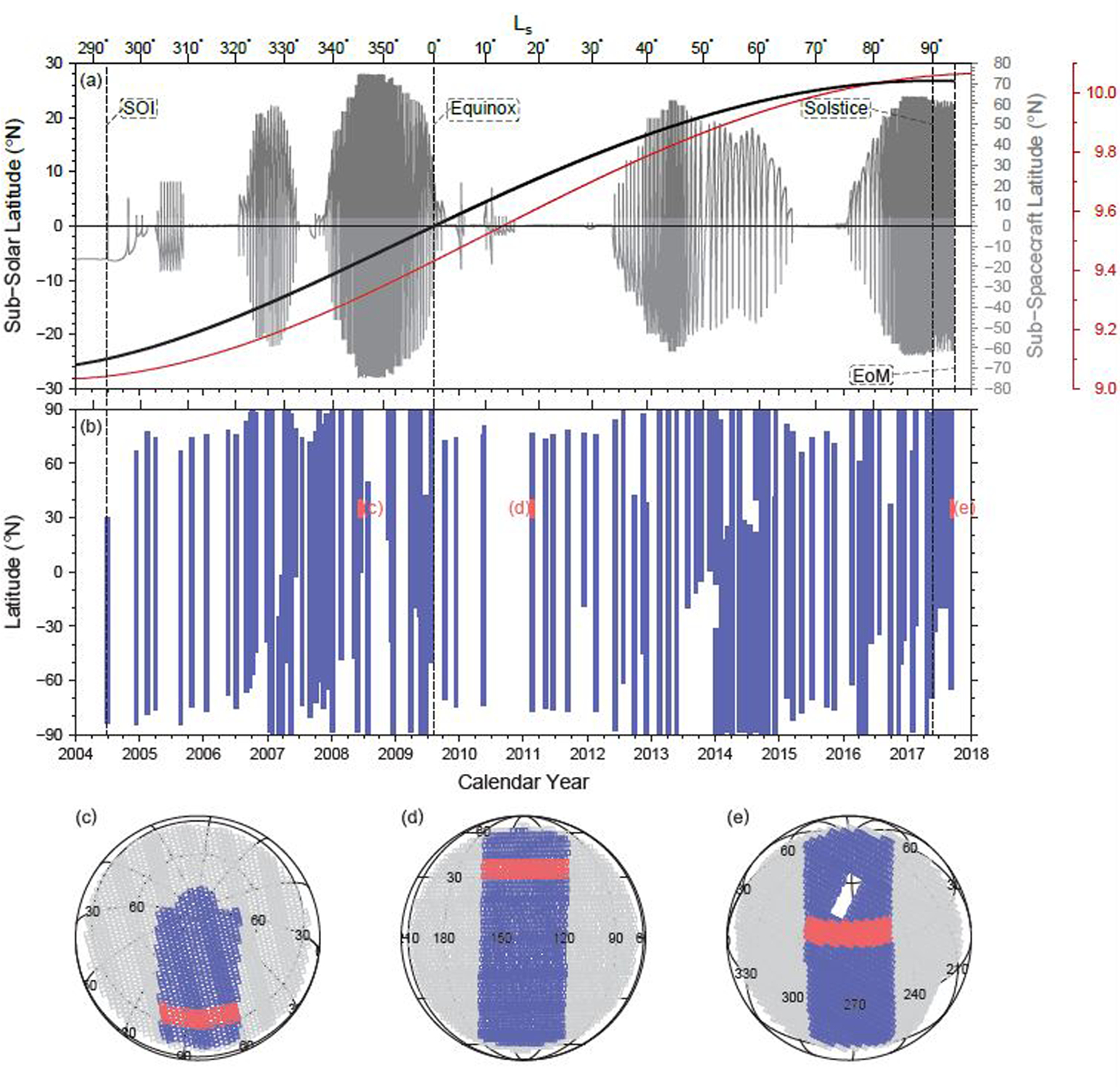
CIRS data summary for the entire Cassini mission. (a) Evolution of sub-solar latitude (black), sub-spacecraft latitude projected onto Saturn (grey), and Sun-Saturn distance throughout the mission (red). Saturn orbit insertion (SOI) until the end of mission (EoM) covers northern winter, northern spring equinox, and northern summer solstice. The complex tour includes four high orbital inclination periods, which give coverage of the north and south poles. (b) Latitude-time coverage of the 2.5 cm−1 resolution CIRS nadir mapping observations. There are several data gaps at the poles, but overall the CIRS dataset has excellent coverage. (c–e) Examples of observation binning to improve signal-to-noise. Grey shows the footprint of all spectra in an observation sequence, blue shows spectra which satisfy emission angle and geometry constraints, and red shows examples of spectra included in a 10° latitude bin (30–40° N). Example bin locations are indicated in (b).
The inversion method is explained in detail in previous papers (Irwin et al., 2008; Teanby, Irwin, et al., 2008; Teanby et al., 2010b, 2006) and is briefly summarised here. Spectra were inverted for temperature and composition using the NEMESIS retrieval code (Irwin et al., 2008), which employs an optimal estimation technique. Partial derivatives of the forward modelled radiances were calculated analytically with respect to each model variable using radiative transfer theory. The temperature and composition were then iteratively adjusted to fit the data, while remaining as close to the a-priori profiles as possible (Irwin et al., 2008).
Here we use a two stage inversion process similar to that in Teanby et al. (2010b). First a continuous temperature profile was retrieved for each binned spectrum using the ν4 methane band in FP4 over the spectral range 1240–1360 cm−1. A latitude- and time-dependent temperature a-priori (supporting text S2) was used as the starting point, with an a-priori error σ varying as a function of latitude θ between σeq=2 K at the equator and σpole=5 K at the poles according to σ = σpole−(σpole−σeq) cos θ. This accounted for the greater uncertainty in polar temperatures compared to the more stable and well constrained equator, where we have the advantage of Huygens probe direct temperature measurements (Fulchignoni et al., 2005). A correlation length of 1.5 atmospheric scale heights was assumed for the off-diagonal elements of the temperature a-priori covariance matrix to ensure a smooth temperature profile was retrieved (Irwin et al., 2008). Second, the temperature was fixed and uniform a-priori gas profiles (supporting text S3) were scaled to provide the best fit to the observed spectra. Example fits to the data are shown in Figure 2 along with the corresponding fitted temperature and composition profiles.
Figure 2.

Example fits to CIRS spectra at 75° N from Cassini’s final Titan flyby (orbit 293). (a) Fit to the ν4 CH4 band in FP4 and (b) retrieved temperature profile used for the fit. (c, e) Fits to the trace gas vibrational features in the FP3 spectrum and (d, f) corresponding trace gas VMR profiles. All gases are assumed to have a uniform abundance profile above the condensation level. This simplified parameterisation is sufficient to fit these data. Note that C2 H4 does not condense under Titan’s atmospheric conditions.
Nadir observation sensitivity is limited to mid-stratosphere to lower mesosphere (∼5–0.1 mbar), with peak information content at ∼1 mbar. Near the winter pole the range of sensitivity is 1–0.01 mbar for cases with a hot stratopause and very cold lower to middle stratosphere. Contribution functions for both these cases are plotted in Teanby, Irwin, et al. (2008) (their Figure 3).
Figure 3.
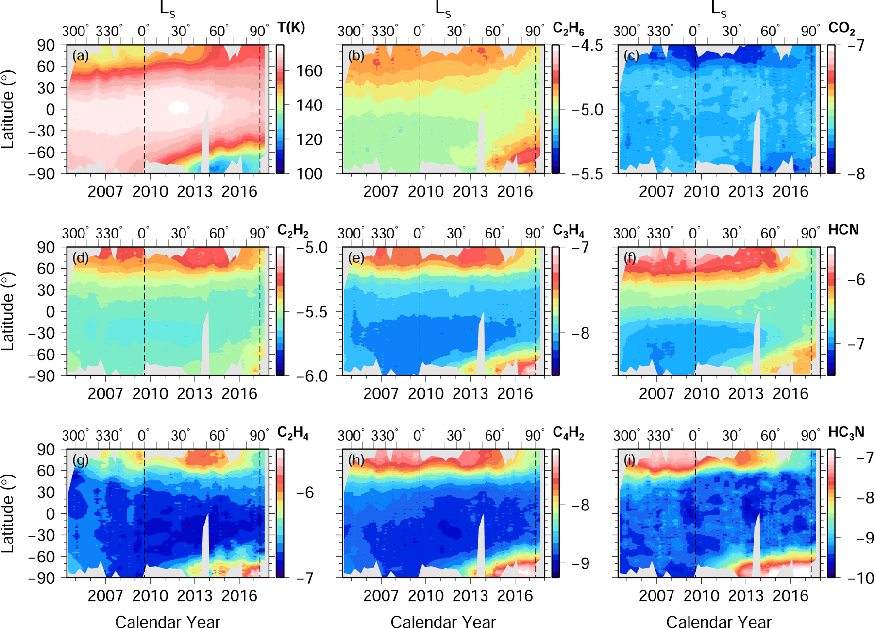
Temperature and composition seasonal latitude variation at the 1 mbar pressure level. Temperature shows a warm equator and cold winter poles, with the south winter pole reaching the coldest temperatures. Composition variations show trace gas enrichment at the winter poles, again with the most extreme enrichment at the southern winter pole. Short-lifetime gases (C4 H2 and HC3 N) have the largest enrichment, whereas the longest lifetime gas (CO2 ) does not vary significantly. North-polar enrichment persists for ∼60–90° of Ls after equinox. Vertical dashed lines show the 2009 northern spring equinox (Ls =0 ) and 2017 northern summer solstice (Ls=90°). The 1 mbar surfaces are fitted to irregularly spaced inversion results using a 2D spline in tension (Smith & Wessel, 1990) with a grid spacing of 0.1 years (∼1° of Ls ) and 1° latitude. Grey areas indicate data gaps. Units of composition are log10 (VMR).
3. Results
Figure 3 shows the latitudinal variation of temperature and composition at the 1 mbar pressure level with season for the entire Cassini mission. Figure 4 shows the seasonal variation in time series form for latitudes 80°S, 50°S, 0°N, 50°N, and 80°N. In this section we briefly discuss gross features of the temperature and composition results. Implications for Titan’s atmosphere are considered in Section 4.
Figure 4.

Seasonal variation of temperature and composition at five latitudes. Temperature is shown at 5, 1, and 0.1 mbar. The 0.1 mbar pressure level is near the stratopause and is most sensitive to seasonal changes; for example cooling of the stratopause hot spot preceding equinox and adiabatic heating from Ls∼60° onwards. Vertical dashed lines show the 2009 northern spring equinox and 2017 northern summer solstice. Points with errors are individual measurements and lines with error envelopes are cubic b-spline fits under tension using a knot spacing of 15° of Ls for 0 and ±50°N, or 30° of Ls for ±80°N where data coverage is sparser (Teanby, 2007).
3.1. Seasonal temperature variations
The mid-stratosphere 1 mbar temperatures shown in Figure 3 are warmest at the equator, with peak temperatures occurring at Ls∼30°. The equatorial temperature maximum moves northward as the season progresses from northern winter to northern summer, from ∼10°S at Ls=293° to ∼0°N from Ls∼30° onwards. Equatorial temperatures at 1 mbar are relatively stable until Ls ∼30°, after which they reduce by ∼5 K between Ls=30–93°. Temperatures at 1 mbar are coldest over the winter poles. The south pole has the coldest observed temperatures at this pressure level, occurring at Ls∼60° in early southern winter.
Figure 4 shows the temperature variation at 5, 1, and 0.1 mbar for comparison. The temperature at 0.1 mbar displays the most seasonal variation, especially near the poles with a ∼20 K pre-equinox cooling at the north pole and a ∼45 K post-equinox cooling and subsequent recovery at the south pole. The 5 mbar temperature exhibits a steady post-equinox decrease for the equator and southern hemisphere, and a steady increase in the northern hemisphere.
3.2. Seasonal composition variations
Seasonal composition variations in Figure 3 are most appropriate for the 1 mbar level, based on contribution functions for the uniform profiles assumed here. Gases display a consistent behaviour, with high concentrations over the poles during winter and approximately constant abundance at the equator, except for CO2, which is roughly constant at all latitudes. The degree of enrichment over the poles depends on the gas species; HC3N and C4H2 show the most extreme polar enrichments (2–3 orders of magnitude), whereas HCN, C2H2, C2H4, C2H6, and C3H4 have more modest enrichments (∼1 order of magnitude or less). HC3N and C4H2 react faster to the seasons than the more modestly enriched species, with HC3N changing the fastest.
Note that absolute VMR values depend on profile assumptions, which can vary with latitude and season. For most gases, which have modest vertical gradients, this effect is small and the absolute VMRs can be considered representative of the stratosphere. However, for short-lifetime gases like HC3N and C4H2 that have very steep vertical gradients, the peak of the contribution function can shift to lower pressures, which leads to an overestimate of the stratospheric abundances (Teanby et al., 2006). Therefore, the uniform profile results presented here should only be used to inspect relative abundance variations as these are robust to profile assumptions. For example, relative abundance comparisons of HC3N for different latitudes and times are valid, but absolute abundance comparisons between HC3N and C2H2 are not valid. This is a fundamental limitation of the CIRS nadir spectra, which are sensitive to a broad pressure range and contain limited vertical information. Where absolute abundances are critical (e.g. for photochemical model profile comparisons) limb viewing data is required (e.g. Teanby et al., 2012; Vinatier et al., 2015).
4. Discussion
4.1. Polar vortex general characteristics
In general, Titan’s stratospheric winter polar vortices are characterised by cold temperatures at 1 mbar, 20–50 K colder than at the equator (Figure 3). These cold temperatures cause a strong thermal gradient, which drives strong circumpolar winds, creates a potential vorticity gradient and mixing barrier, and effectively isolates the polar airmass from more equatorial latitudes (Achterberg et al., 2008; Achterberg et al., 2011; Flasar et al., 2005; Teanby, de Kok, et al., 2008). This allows subsiding air masses to enrich the polar stratosphere in trace gas species, which are advected down from the upper atmosphere photochemical production zone where they are more abundant (Teanby et al., 2009). Subsidence causes significant adiabatic heating at low pressures and leads to a hot stratopause over the winter pole (Achterberg et al., 2008; Teanby et al., 2017). Trace gas enrichment is largest for short-lifetime gases (HC3N and C4H2), which tend to have steeper vertical gradients and are more susceptible to enrichment by subsidence (Teanby et al., 2009). The polar isolation is also most effective for short lifetime species, whereas intermediate lifetime species such as HCN and C2H2 can be mixed across the vortex barrier and leach to lower latitudes (Teanby, de Kok, et al., 2008). Longer-lifetime species are less enriched, with the very long lifetime species CO2 showing virtually no variation, indicating a more uniform vertical profile consistent with a lifetime much longer than any dynamical timescale. This general picture is confirmed by our new results (Figures 3–4), but our longer time series covering the whole Cassini mission (Ls=293–93°) allows further insight into vortex break-up and formation processes by observing both north and south poles (Sections 4.2–4.3).
4.2. North-polar vortex evolution
The northern winter vortex was already well established when Cassini arrived at Ls=293° and extended from the north pole down to ∼45°N. Initially the 1 mbar temperatures were around 140 K, compared to 170 K at the equator, but had warmed to 160 K by the end of the mission at Ls=93° (Figure 4). As the mission progressed the vortex shrank in extent, being limited to latitudes north of 60°N from Ls=20° onwards (Figure 3).
Our results show the north-polar vortex endured well beyond the northern spring equinox (Ls=0°), maintaining cold temperatures and enriched trace gas abundances until at least late spring (Ls∼60°). After this point vortex dissipation was first visible in temperature and short-lifetime gases (HC3N and C4H2) as a warming and abundance reduction. Early stages of vortex break-up were also visible in a subset of observations taken at 70°N before mid-2016 (Ls<80°) by Coustenis et al. (2018).
The hot stratopause at 0.1 mbar driven by adiabatic heating was already cooling at Ls∼320° and had stabilised in temperature by Ls=0°, indicating a weakening in north-polar subsidence. The mid-stratosphere at 1 mbar was slower to respond because of the longer radiative time constant, with temperatures increasing more gradually by ∼20 K between Ls=0–90°, due to increased insolation. These observations indicate weakening of the vortex. A reduction in HC3N and C4H2 abundance starting at Ls∼50° is the first sign of vortex break-up. Longer-lifetime species dissipated over the proceeding Ls∼60–90° period. There was a north-polar data gap at Ls∼70°, but the final orbits of Cassini around northern summer solstice (Ls=90°) showed north-polar gases had attained almost equatorial abundances and vortex break-up was complete.
Interestingly, our results show that after vortex break-up, spreading of air enriched in trace gases to lower latitudes did not occur (Figure 3). This shows that polar gas depletion by small-scale cross-latitude mixing, which would enhance trace gas abundances at sub-polar latitudes post-vortex break-up, is small compared to other effects. Further-more, this suggests the bulk of stratospheric trace gas loss must be due to a combination of large-scale dynamics and photochemistry. In this scenario, upwelling from the reversed meridional Hadley circulation would advect trace gas depleted air from lower latitudes into the north-polar mid-stratosphere, leading to a reduction in abundances. Photochemical loss, enabled by increasing insolation after equinox, could also contribute to a reduction in polar stratospheric trace gas abundance during northern spring.
4.3. South-polar vortex evolution
South-polar nadir observations have a data gap after equinox, but previous limb viewing observations showed the south-polar winter vortex formed almost immediately after northern spring equinox (Teanby et al., 2012; Vinatier et al., 2015). Early southern winter vortex temperatures dramatically cooled to ∼120 K during Ls=0–60° at 1 mbar. This is much colder than was observed in the mid-winter north-polar vortex and can explain the high altitude HCN and C6H6 ice clouds observed by de Kok et al. (2014) and Vinatier et al. (2018). The extremely cold temperatures could be caused by enhanced radiative cooling from enriched trace gases, which are effective infrared coolers (Bézard et al., 2018; Teanby et al., 2017). In the early stages of vortex formation this cooling was not mitigated by significant adiabatic heating as the reversed meridional Hadley circulation was initially quite sluggish (Teanby et al., 2017; Teanby et al., 2012). It is also possible that enhancement of infrared cooling gases may form a radiative feedback, contributing to establishing the reversed circulation (Teanby et al., 2017). Post-equinox the south-polar vortex continued to grow and by Ls∼90° it was similar in extent to the mid-winter northern vortex, reaching 45°S. It is likely that the early northern winter vortex also exhibited this behaviour, but this phase would occur for Ls=180–270° prior to Cassini’s arrival, so remains unobserved.
For the shortest lifetime gases (e.g. HC3N and C4H2), there appeared to be some overshoot of enrichment during vortex formation, with south-polar abundances being enhanced by up to an order of magnitude compared to those observed in the mid-winter north-polar vortex. This can be seen in Figure 4, with abundances peaking around Ls=60–90° at 80°S. Therefore, the largest winter polar trace gas enrichments occured between equinox and winter solstice. This effect was also visible in limb observations (Teanby et al., 2017; Teanby et al., 2012; Vinatier et al., 2015), but with peak abundances occurring earlier (Ls <60°) at high altitude (>300 km, <0.1 mbar) and later (Ls >60°) at low altitude (<300 km, >0.1 mbar). Near the end of the mission (Ls=93°), temperatures and abundances appeared to be trending towards those observed in northern mid-winter (Figure 4). This suggests north and south-polar vortices have similar temperatures and chemistry at similar seasonal phases.
One potential explanation for the extreme south-polar enrichments observed during Ls=0–90° requires a combination of photochemistry, insolation, and dynamics. Close to equinox, upper atmosphere abundances of trace gases were highest because the southern hemisphere was just exiting summer – a period of relatively high insolation and photochemical production. Then, after equinox, as the circulation reversed and subsidence developed, the trace gas vertical profiles were advected downwards, leading to large stratospheric enrichments. However, as the season progressed, overall insolation in the southern hemisphere steadily decreased, in turn reducing upper atmosphere photochemical production, which led to lower trace gas abundances at high altitude. This reduced the supply of trace gases into the vortex and led to less extreme polar enrichments. The latitude extent of the vortex also could play a role. Initially the vortex had a small latitude extent, so drew air from the upper atmosphere directly above the pole, which had constant illumination above 300 km altitude throughout winter, but as the vortex grew the air in the vortex was sourced from a wider region of the southern hemisphere, which had lower insolation and reduced upper atmosphere trace gas abundances. This conceptual explanation would need a coupled GCM and photochemical model to investigate further.
4.4. Equatorial temperatures
The 1 mbar temperature maximum was skewed towards the sub-solar point, but stayed within 10° of the equator. The temperature at 5 mbar exhibited a steady 5 K cooling from Ls=293–93°, which was caused by the increase in Sun-Saturn distance over the mission (Figure 1a). This effect was also clearly observed in the lower stratosphere (10–30 mbar) in previous analysis of far-infrared FP1 spectra (Sylvestre, Teanby, Vinatier, Lebonnois, & Irwin, 2019). At lower pressures (∼1–0.1 mbar) dynamics had a larger effect on the temperature (Bézard et al., 2018) and the effect of the increasing Sun-Saturn distance was less apparent.
5. Conclusions
Cassini CIRS nadir mapping observations of Titan were analysed for the entire mission duration, which ran from northern mid-winter (Ls=293°) until just after northern summer solstice (Ls=93°), to obtain seasonal-latitude variation maps at the 1 mbar pressure level. The equatorial composition was stable for all the species analysed, whereas the mid-latitudes and polar regions exhibited significant variability.
Winter vortices were observed at both poles with cold temperatures and isolated air masses enriched in trace gas species. The enrichments were largest for short-lifetime gases and more modest for those with longer lifetimes, in keeping with previous studies (Teanby et al., 2009, 2010a). However, early and mid-winter vortices evidently had very different properties. When newly formed, the south-polar vortex was significantly more enriched in trace gases and achieved colder temperatures than its established northern counterpart. Trace gas abundances were up to an order of magnitude greater at the southern early-winter pole than the northern mid-winter pole. This could be due to enhanced radiative cooling from trace gases combined with a relatively weak subsidence and initially steeper photochemical profiles during vortex formation. This suggests early vortex temperature structure was dominated by radiative cooling, whereas mid-winter vortex temperatures were dominated by subsidence-driven adiabatic heating.
Dissipation of the north-polar vortex was a gradual process and was only complete ∼90° of Ls after equinox. Gas enrichments did not appear to spread from high to low latitudes during vortex break-up, suggesting that photochemistry and depletion due to large-scale dynamics related to the meridional circulation (upwelling) were more important loss mechanisms than small-scale cross-latitude mixing. Near the end of the mission the temperature and composition of the south-polar vortex were trending towards those observed in the north at the start of the mission. However, as the Cassini dataset covers ∆Ls=160°, we are 20° of Ls short of a complete half Titan year record. Therefore, it is not possible to definitively confirm that north and south poles reach equivalent states for equivalent seasons, although a short extrapolation of the data suggests seasonal equivalence is very likely. This implies temperature and composition differences between the mid-winter north-polar vortex and early-winter south-polar vortex were primarily due to seasonal phase, not any hemispheric asymmetry.
Over the next few years it will be important to observe the north-polar temperature and composition using ground and space based facilities such as ALMA and JWST. ALMA has already produced moderate resolution latitude maps, which have the potential to complete the CIRS record at high northern latitudes (Thelen et al., 2019, 2018). Unfortunately, with the loss of Cassini, the winter poles can no longer be observed until we next visit Titan.
Supplementary Material
Key Points:
Early and mid-winter polar vortices have distinct behaviours and different dominant processes.
Large-scale dynamics and photochemistry determine polar chemical evolution during vortex break-up.
The northern winter vortex persisted until late-spring, with break-up completed by mid-summer.
Acknowledgments
NAT, MS, JS, and PGJI were funded by the UK Science and Technology Facilities Council (STFC). CAN was supported by the NASA Cassini project and the NASA Astrobiology Institute. SV was funded by the French Centre National d’Etudes Spatiales (CNRS). The Cassini CIRS observations, summarised in Table S1, are publicly available from NASA’s Planetary Data System at https://pds.nasa.gov. Temperature and composition results from this paper are available in supporting datasets S1 and S2, with a gridded NetCDF format product in dataset S3.
Footnotes
Publisher's Disclaimer: This article has been accepted for publication and undergone full peer review but has not been through the copyediting, typesetting, pagination and proofreading process which may lead to differences between this version and the Version of Record.
References
- Achterberg RK, Conrath BJ, Gierasch PJ, Flasar FM, & Nixon CA (2008). Titan’s middle-atmospheric temperatures and dynamics observed by the Cassini Composite Infrared Spectrometer. Icarus, 194, 263–277. [Google Scholar]
- Achterberg RK, Gierasch PJ, Conrath BJ, Flasar FM, & Nixon CA (2011). Temporal variations of Titan’s middle-atmospheric temperatures from 2004 to 2009 observed by Cassini/CIRS. Icarus, 211, 686–698. [Google Scholar]
- Bézard B (2014). The composition of titan’s atmosphere In Müller-Wodarg I, Griffith CA, Lellouch E, & Cravens TE (Eds.), Titan: Interior, surface, atmosphere, and space environment (pp. 158–189). Cambridge Univ. Press. [Google Scholar]
- Bézard B, Coustenis A, & McKay CP (1995). Titan’s stratospheric temperature asymmetry - a radiative origin. Icarus, 113, 267–276. [DOI] [PubMed] [Google Scholar]
- Bézard B, Vinatier S, & Achterberg RK (2018). Seasonal radiative modeling of Titan’s stratospheric temperatures at low latitudes. Icarus, 302, 437–450. [Google Scholar]
- Borysow A (1991). Modelling of collision-induced infrared-absorption spectra of H2−H2 pairs in the fundamental band at temperatures from 20K to 300K. Icarus, 92 (2), 273–279. [Google Scholar]
- Borysow A, & Frommhold L (1986a). Collision-induced rototranslational absorption spectra of N2−N2 pairs for temperatures from 50 to 300K. Astrophys. J, 311, 1043–1057. [Google Scholar]
- Borysow A, & Frommhold L (1986b). Theoretical collision-induced rototranslational absorption spectra for modeling Titan’s atmosphere: H2−N2 pairs. Astrophys. J, 303, 495–510. [Google Scholar]
- Borysow A, & Frommhold L (1986c). Theoretical collision-induced rototranslational absorption spectra for the outer planets: H2−CH4 pairs. Astrophys. J, 304, 849–865. [Google Scholar]
- Borysow A, & Frommhold L (1987). Collision-induced rototranslational absorption spectra of CH4−CH4 pairs at temperatures from 50 to 300K. Astrophys. J, 318, 940–943. [Google Scholar]
- Borysow A, & Tang C (1993). Far infrared CIA spectra of N2−CH4 pairs for modeling of Titan’s atmosphere. Icarus, 105, 175–183. [Google Scholar]
- Coustenis A, Achterberg RK, Conrath BJ, Jennings DE, Marten A, Gautier D, … Courtin R (2007). The composition of Titan’s stratosphere from Cassini/CIRS mid-infrared spectra. Icarus, 189, 35–62. [Google Scholar]
- Coustenis A, & Bézard B (1995). Titan’s atmosphere from Voyager infrared observations. IV. spatial variations of temperature and composition. Icarus, 115, 126–140. [Google Scholar]
- Coustenis A, Bézard B, Gautier D, Marten A, & Samuelson R (1991). Titan’s atmosphere from Voyager infrared observations. III. vertical distributions of hydrocarbons and nitriles near Titan’s north-pole. Icarus, 89, 152–167. [Google Scholar]
- Coustenis A, Jennings DE, Achterberg RK, Bampasidis G, Lavvas P, Nixon CA, … Flasar FM (2016). Titan’s temporal evolution in stratospheric trace gases near the poles. Icarus, 270, 409–420. [Google Scholar]
- Coustenis A, Jennings DE, Achterberg RK, Bampasidis G, Nixon CA, Lavvas P, … Flasar FM (2018). Seasonal Evolution of Titan’s Stratosphere Near the Poles. Astrophys. J. Lett, 854, L30 10.3847/2041-8213/aaadbd [DOI] [PMC free article] [PubMed] [Google Scholar]
- Coustenis A, Nixon C, Achterberg R, Lavvas P, Vinatier S, Teanby N, … Romani P (2010). Titan trace gaseous composition from CIRS at the end of the Cassini-Huygens prime mission. Icarus, 207, 461–476. [Google Scholar]
- de Kok RJ, Teanby NA, Maltagliati L, Irwin PGJ, & Vinatier S (2014). HCN ice in Titan’s high-altitude southern polar cloud. Nature, 514, 65–67. [DOI] [PubMed] [Google Scholar]
- de Kok R, Irwin PGJ, Teanby NA, Lellouch E, Bezard B, Vinatier S, … Taylor FW (2007). Oxygen compounds in Titan’s stratosphere as observed by Cassini CIRS. Icarus, 186, 354–363. [Google Scholar]
- de Kok R, Irwin PGJ, Teanby NA, Nixon CA, Jennings DE, Fletcher L, … Taylor FW (2007). Characteristics of Titan’s stratospheric aerosols and condensate clouds from Cassini CIRS far-infrared spectra. Icarus, 191, 223–235. [Google Scholar]
- de Kok R, Irwin PGJ, Teanby NA, Vinatier S, Negrão A, Osprey S, … A., C. (2010). A tropical haze band in Titan’s stratosphere. Icarus, 207, 485–490. [Google Scholar]
- Dobrijevic M, Hébrard E, Loison JC, & Hickson KM (2014). Coupling of oxygen, nitrogen, and hydrocarbon species in the photochemistry of Titan’s atmosphere. Icarus, 228, 324–346. [Google Scholar]
- Flasar FM, Achterberg RK, Conrath BJ, Gierasch PJ, Kunde VG, Nixon CA, … Wishnow EH (2005). Titan’s atmospheric temperatures, winds, and composition. Science, 308, 975–978. [DOI] [PubMed] [Google Scholar]
- Flasar FM, Kunde VG, Abbas MM, Achterberg RK, Ade P, Barucci A, … Taylor FW (2004). Exploring the Saturn system in the thermal infrared: The Composite Infrared Spectrometer. Space Sci. Rev, 115, 169–297. [Google Scholar]
- Fulchignoni M, Ferri F, Angrilli F, Ball AJ, Bar-Nun A, Barucci MA, … Zarnecki JC (2005). In situ measurements of the physical characteristics of Titan’s environment. Nature, 438, 785–791. [DOI] [PubMed] [Google Scholar]
- Haynes WM (Ed.). (2011). CRC handbook of chemistry and physics (92nd ed.). Bosa Roca: Taylor & Francis Inc. [Google Scholar]
- Hörst SM, Vuitton V, & Yelle RV (2008). Origin of oxygen species in Titan’s atmosphere. J. Geophys. Res, 113, E10006. [Google Scholar]
- Hourdin F, Talagrand O, Sadourny R, Courtin R, Gautier D, & McKay C (1995). Numerical simulation of the general circulation of the atmosphere of Titan. Icarus, 117, 358–374. [DOI] [PubMed] [Google Scholar]
- Irwin P, Teanby N, de Kok R, Fletcher L, Howett C, Tsang C, … Parrish P (2008). The NEMESIS planetary atmosphere radiative transfer and retrieval tool. J. Quant. Spectro. Rad. Trans, 109, 1136–1150. [Google Scholar]
- Jacquinet-Husson N, Armante R, Scott NA, Chédin A, Crépeau L, Boutammine C, … Makie A (2016). The 2015 edition of the GEISA spectroscopic database. J. Mol. Spectrosc, 327, 31–72. [Google Scholar]
- Jennings DE, Flasar FM, Kunde VG, Nixon CA, Segura ME, Romani PN, … Ferrari C (2017). Composite infrared spectrometer (CIRS) on Cassini. Appl. Opt, 56 10.1364/ao.56.005274 [DOI] [PubMed] [Google Scholar]
- Krasnopolsky VA (2009). A photochemical model of Titan’s atmosphere and ionosphere. Icarus, 201, 226–256. [Google Scholar]
- Kunde V, Ade P, Barney R, Bergman D, Bonnal J, Borelli R, … Yun D (1996). Cassini infrared Fourier spectroscopic investigation. Proc. Soc. Photo-Opt. Instrum. Eng, 2803, 162–177. [Google Scholar]
- Lavvas PP, Coustenis A, & Vardavas IM (2008). Coupling photochemistry with haze formation in Titan’s atmosphere, Part II: Results and validation with Cassini/Huygens data. Plan. & Space Sci, 56, 67–99. [Google Scholar]
- Le Mouélic S, Rodriguez S, Robidel R, Rousseau B, Seignovert B, Sotin C, … Cornet T (2018). Mapping polar atmospheric features on Titan with VIMS: From the dissipation of the northern cloud to the onset of a southern polar vortex. Icarus, 311, 371–383. 10.1016/j.icarus.2018.04.028 [DOI] [Google Scholar]
- Lebonnois S, Burgalat J, Rannou P, & Charnay B (2012). Titan global climate model: a new 3-dimensional version of the IPSL Titan GCM. Icarus, 218, 707–722. [Google Scholar]
- Lebonnois S, Flasar FM, Tokano T, & Newman CE (2014). The general circulation of titan’s lower and middle atmosphere. In Müller-Wodarg I, Griffith CA, Lellouch E, & Cravens TE (Eds.), Titan: Interior, surface, atmosphere, and space environment (pp. 122–157). Cambridge Univ. Press. [Google Scholar]
- Loison JC, Hébrard E, Dobrijevic M, Hickson KM, Caralp F, Hue V, … Bénilan Y (2015). The neutral photochemistry of nitriles, amines and imines in the atmosphere of Titan. Icarus, 247, 218–247. [Google Scholar]
- Lora JM, Lunine JI, & Russell JL (2015). GCM simulations of Titan’s middle and lower atmosphere and comparison to observations. Icarus, 250, 516–528. 10.1016/j.icarus.2014.12.030 [DOI] [Google Scholar]
- Newman CE, Lee C, Lian Y, Richardson MI, & Toigo AD (2011). Stratospheric superrotation in the TitanWRF model. Icarus, 213, 636–654. [Google Scholar]
- Niemann HB, Atreya SK, Demick JE, Gautier D, Haberman JA, Harpold DN, … Raulin F (2010). Composition of Titan’s lower atmosphere and simple surface volatiles as measured by the Cassini-Huygens probe gas chromatograph mass spectrometer experiment. J. Geophys. Res, 115, E12006. [Google Scholar]
- Nixon CA, Teanby NA, Calcutt SB, Aslam S, Jennings DE, Kunde VG, … Smith MD (2009). Infrared limb sounding of Titan with the Cassini Composite Infrared Spectrometer: effects of the mid-IR detector spatial responses. Appl. Opt, 48, 1912–1925. [DOI] [PubMed] [Google Scholar]
- Rothman L, Gordon I, Babikov Y, Barbe A, Benner DC, Bernath P, … Wagner G (2013). The HITRAN2012 molecular spectroscopic database. J. Quant. Spectro. Rad. Trans, 130, 4–50. [Google Scholar]
- Smith WHF, & Wessel P (1990). Gridding with continuous curvature splines in tension. Geophysics, 55, 293–305. [Google Scholar]
- Sylvestre M, Teanby NA, Vinatier S, Lebonnois S, & Irwin PGJ (2018). Seasonal evolution of C2N2, C3H4, and C4H2 abundances in Titan’s lower stratosphere. Astron. Astrophys, 609, A64 10.1051/0004-6361/201630255 [DOI] [Google Scholar]
- Sylvestre M, Teanby NA, Vinatier S, Lebonnois S, & Irwin PGJ (2019). Seasonal evolution of temperatures in Titan’s lower stratosphere. Icarus, in press. doi: arXiv:1902.01841 [DOI] [PMC free article] [PubMed]
- Teanby NA (2007). Constrained smoothing of noisy data using splines in tension. Math. Geol, 39, 419–434. [Google Scholar]
- Teanby NA, Bézard B, Vinatier S, Sylvestre M, Nixon CA, Irwin PGJ, … Flasar FM (2017). The formation and evolution of titan’s winter polar vortex. Nature Comms, 8 (1), 1586. [DOI] [PMC free article] [PubMed] [Google Scholar]
- Teanby NA, de Kok R, Irwin PGJ, Osprey S, Vinatier S, Gierasch PJ, … Calcutt SB (2008). Titan’s winter polar vortex structure revealed by chemical tracers. J. Geophys. Res, 113, E12003. [Google Scholar]
- Teanby NA, Irwin PGJ, de Kok R, & Nixon CA (2009). Dynamical implications of seasonal and spatial variations in Titan’s stratospheric composition. Phil. Trans. R. Soc. Lond. A, 367, 697–711. [DOI] [PubMed] [Google Scholar]
- Teanby NA, Irwin PGJ, de Kok R, Nixon CA, Coustenis A, Royer E, … Taylor FW (2008). Global and temporal variations in hydrocarbons and nitriles in Titan’s stratosphere for northern winter observed by Cassini/CIRS. Icarus, 193, 595–611. [Google Scholar]
- Teanby NA, Irwin PGJ, de Kok R, & Nixon CA (2010a). Mapping Titan’s HCN in the far infra-red: implications for photochemistry. Faraday Discussions, 147, 51–64. [DOI] [PubMed] [Google Scholar]
- Teanby NA, Irwin PGJ, de Kok R, & Nixon CA (2010b). Seasonal changes in Titan’s polar trace gas abundance observed by Cassini. Astrophys. J. Lett, 724, L84–L89. [Google Scholar]
- Teanby NA, Irwin PGJ, de Kok R, Nixon CA, Coustenis A, Bézard B, … Taylor FW (2006). Latitudinal variations of HCN, HC3N, and C2N2 in Titan’s stratosphere derived from Cassini CIRS data. Icarus, 181, 243–255. [Google Scholar]
- Teanby NA, Irwin PGJ, de Kok R, Vinatier S, Bézard B, Nixon CA, … Taylor FW (2007). Vertical profiles of HCN, HC3N, and C2H2 in Titan’s atmosphere derived from Cassini/CIRS data. Icarus, 186, 364–384. [Google Scholar]
- Teanby NA, Irwin PGJ, Nixon CA, de Kok R, Vinatier S, Coustenis A, … Flasar FM (2012). Active upper-atmosphere chemistry and dynamics from polar circulation reversal on Titan. Nature, 491, 732–735. 10.1038/nature11611 [DOI] [PubMed] [Google Scholar]
- Thelen AE, Nixon CA, Chanover NJ, Cordiner MA, Molter EM, Teanby NA, … Charnley SB (2019). Abundance measurements of Titan’s stratospheric HCN, HC3N, C3H4, and CH3CN from ALMA observations. Icarus, 319, 417–432. 10.1016/j.icarus.2018.09.023 [DOI] [Google Scholar]
- Thelen AE, Nixon CA, Chanover NJ, Molter EM, Cordiner MA, Achterberg RK, … Charnley SB (2018). Spatial variations in Titan’s atmospheric temperature: ALMA and Cassini comparisons from 2012 to 2015. Icarus, 307, 380–390. 10.1016/j.icarus.2017.10.042 [DOI] [Google Scholar]
- Tomasko MG, Doose L, Engel S, Dafoe LE, West R, Lemmon M, … See C (2008). A model of Titan’s aerosols based on measurements made inside the atmosphere. Plan. & Space Sci, 56, 669–707. [Google Scholar]
- Vinatier S, Bézard B, de Kok R, Anderson CM, Samuelson RE, Nixon CA, … Kunde V (2010). Analysis of Cassini/CIRS limb spectra of Titan acquired during the nominal mission. II: aerosol extinction profiles in the 600 – 1420 cm−1 spectral range. Icarus, 210, 852–866. [Google Scholar]
- Vinatier S, Bézard B, Fouchet T, Teanby NA, de Kok R, Irwin PGJ, … Coustenis A (2007). Vertical abundance profiles of hydrocarbons in Titan’s atmosphere at 15°S and 80°N retrieved from Cassini/CIRS spectra. Icarus, 188, 120–138. [Google Scholar]
- Vinatier S, Bézard B, Lebonnois S, Teanby NA, Achterberg RK, Gorius N, … Flasar FM (2015). Seasonal variations in Titan’s middle atmosphere during the northern spring derived from Cassini/CIRS observations. Icarus, 250, 95–115. [Google Scholar]
- Vinatier S, Bézard B, Nixon CA, Mamoutkine A, Carlson RC, Jennings DE, … Kunde VG (2010). Analysis of Cassini/CIRS limb spectra of Titan acquired during the nominal mission I. hydrocarbons, nitriles and CO2 vertical mixing ratio profiles. Icarus, 205, 559–570. [Google Scholar]
- Vinatier S, Rannou P, Anderson CM, Bézard B, de Kok R, & Samuelson RE (2012). Optical constants of Titan’s stratospheric aerosols in the 70–1500 cm−1 spectral range constrained by Cassini/CIRS observations. Icarus, 219, 5–12. [Google Scholar]
- Vinatier S, Schmitt B, Bézard B, Rannou P, Dauphin C, de Kok R, … Flasar FM (2018). Study of Titan’s fall southern stratospheric polar cloud composition with Cassini/CIRS: Detection of benzene ice. Icarus, 310, 89–104. 10.1016/j.icarus.2017.12.040 [DOI] [Google Scholar]
- Vuitton V, Yelle RV, Klippenstein SJ, Hörst SM, & Lavvas P (2018). Simulating the density of organic species in the atmosphere of Titan with a coupled ion-neutral photochemical model. Icarus, in press, 10.1016/j.icarus.2018.06.013. [DOI]
- West RA, Seignovert B, Rannou P, Dumont P, Turtle EP, Perry J, … Ovanessian A (2018). The seasonal cycle of Titan’s detached haze.ss Nature Astronomy, 2, 495–500. 10.1038/s41550-018-0434-z [DOI] [Google Scholar]
- Wilson EH, & Atreya SK (2004). Current state of modeling the photochemistry of Titan’s mutually dependent atmosphere and ionosphere. J. Geophys. Res, 109, E06002. [Google Scholar]
Associated Data
This section collects any data citations, data availability statements, or supplementary materials included in this article.