Abstract
The increasing interest in bioactive peptides with therapeutic potentials has been reflected in a large variety of biological databases published over the last years. However, the knowledge discovery process from these heterogeneous data sources is a nontrivial task, becoming the essence of our research endeavor. Therefore, we devise a unified data model based on molecular similarity networks for representing a chemical reference space of bioactive peptides, having an implicit knowledge that is currently not explicitly accessed in existing biological databases. Indeed, our main contribution is a novel workflow for the automatic construction of such similarity networks, enabling visual graph mining techniques to uncover new insights from the “ocean” of known bioactive peptides. The workflow presented here relies on the following sequential steps: (i) calculation of molecular descriptors by applying statistical and aggregation operators on amino acid property vectors; (ii) a two-stage unsupervised feature selection method to identify an optimized subset of descriptors using the concepts of entropy and mutual information; (iii) generation of sparse networks where nodes represent bioactive peptides, and edges between two nodes denote their pairwise similarity/distance relationships in the defined descriptor space; and (iv) exploratory analysis using visual inspection in combination with clustering and network science techniques. For practical purposes, the proposed workflow has been implemented in our visual analytics software tool (http://mobiosd-hub.com/starpep/), to assist researchers in extracting useful information from an integrated collection of 45120 bioactive peptides, which is one of the largest and most diverse data in its field. Finally, we illustrate the applicability of the proposed workflow for discovering central nodes in molecular similarity networks that may represent a biologically relevant chemical space known to date.
Subject terms: Data mining, Protein analysis, Computational biology and bioinformatics
Introduction
During the last years, a growing interest has emerged for the development of Bioactive Peptides (BPs) as potential drugs impacting on human health1,2. As a consequence, a lot of BPs and their biological annotations have been collected from the literature into a large variety of biological databases, providing a valuable ground for knowledge discovery. Naturally, the domain experts in the field of biomedical research need to mine knowledge hidden in those heterogeneous data sources. However, to exploit the available data, most of the previous reports3–6 are primarily focused on the field of supervised machine learning for building predictive models from a set of training instances. These supervised based models are very suitable to predict the biological activities for new molecules whose functions to be predicted are unknown. By contrast, in unsupervised methods, the input data are not labeled with the corresponding outcome, and there is no response to supervise the learning process. So, in this other field of machine learning, the goal is finding interpretable associations and patterns among available data elements.
In this report, we focus on employing unsupervised learning methods for turning existing data of BPs into information not appreciated before. As a foundation for this task, we already have introduced two valuable resources: starPepDB and starPep toolbox7. StarPepDB is an integrated graph database of existing individual databases for a better understanding of the universe of BPs. This comprehensive graph database is one of the largest and most diverse data in its field. It is comprised mainly of 45,120 nodes representing peptide compounds, while additional nodes are connected to these primary nodes for describing metadata, i.e., biological annotations. Moreover, the software named starPep toolbox helps researchers to understand the integrated data through visual network analysis.
Now we continue to extend the implemented visual analysis process to let the end-users gain insight into a graph-based representation of chemical space for studying BPs. Whereas the term chemical space refers to the ensemble of all possible molecules, either natural or synthetically accessible product8,9, a realistic representation focuses on confined regions of such theoretical space. Still, chemical space is so vast that its complete enumeration and visual inspection goes beyond human comprehension. Nonetheless, not all likely compounds are biologically active, and the biologically relevant chemical space is where the bioactive compounds reside8. Thus, the analysis and visualization of chemical space covered by known bioactive peptides (those reported thus far) may play an essential role in decision-making when searching for new peptide-based drugs10,11.
To visualize a chemical space, one of the most common approaches has been a coordinate-based map12, where a set of numerical features (descriptors) characterizes each compound. That is, mathematically, for each chemical compound corresponds a point in a multi-dimensional descriptor space that requires a dimensionality reduction technique for a proper visualization in 2D or 3D maps. For instance, Principal Component Analysis13 (PCA) is a popular technique that seeks a small number of principal components expressed as a linear combination of original features, explaining as much of data variability as possible. In this way, the 2D (3D) map may project the information contained in two (three) of the first principal components of descriptor space, ending in a loss of information.
As an alternative to the coordinate-based map, the so-called Chemical Space Networks (CSNs)14–16 have been proposed as coordinate-free representations for analyzing and visualizing the chemical space without reducing dimensionality. In such CSNs, nodes represent molecular entities while an edge may indicate a similarity relationship between two compounds. A key point of these networks relies on the potential application of graph-based algorithms, which can be used in combination with interactive visualization to enable the domain-expert in the field of Biomedical research to find previously unknown and useful information17,18.
Note that the interactive visualization aims to incorporate the human factor in a process that has been called the Visual Information Seeking Mantra19: overview first, zoom and filter, then details-on-demand. For instance, under this mantra, the interactive visual interface firstly provides an overview of the chemical space. Secondly, the user focuses on molecules of interest and filter out uninteresting peptide compounds. Then, to gain a better understanding of the data, the user accesses only the details of the interesting molecules.
As user interaction relies on a visual representation of chemical space, mapping the raw data of BPs into a multi-dimensional descriptor space should be robust and not accidental to derive consistent conclusions. A grand challenge is to find the most appropriate chemical space representation since there are many different ways of coding molecules to denote the descriptor space, and it is unknown which set of MDs is the best one. So, the success of the visual exploration approach depends on two main aspects: (i) a particular choice of molecular descriptors (MDs), and (ii) proper visualization techniques to display information related to the chosen MDs. Nonetheless, even in cases where the chemical space visualization is unclear, we argue that the interactive exploration, in combination with suitable algorithms may help humans to understand and reason about the chemical data under consideration.
With the study presented here, we tackle the automatic construction of molecular similarity networks for navigating and mining a chemical reference space from our comprehensive collection of BPs. In such molecular similarity networks, each node representing BPs is characterized by a set of molecular descriptors, and edges between nodes denote their pairwise similarity/distance relationships. Once this meaningful network has been created, it can provide insight into drug design for decision-makers20,21.
Results
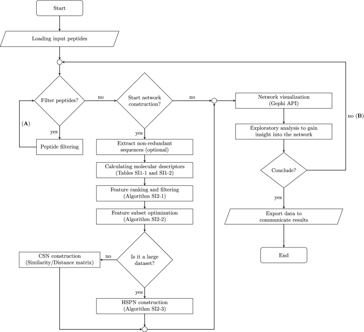
The corresponding steps of a proposed workflow (Fig. 1) have been implemented in our visual analytics software starPep toolbox7 (http://mobiosd-hub.com/starpep/), intended to be used by researchers. As described next, we experimented with the proposed workflow for assessing and tuning the automatic construction of similarity networks from raw amino acid sequences of BPs. We also illustrate the usage of the proposed workflow for turning known BPs into information that is hidden in the existing biological databases. For instance, we generated molecular similarity networks for finding out central nodes that may represent a biologically relevant chemical space of anticancer peptides.
Figure 1.
A flow diagram guiding the automatic construction and visual graph mining of similarity networks. The similarity network can be automatically generated for the first time and just reused, or even it could be regenerated after that. Whereas the mining task is made up of two nested loops, in order, from the most internal to the most external: (A) data manipulation loop, and (B) visual feedback loop. This figure has been created using the package TikZ (version 0.9f 2018-11-19) in Latex, available at https://www.ctan.org/pkg/tikz-cd.
Comparative study of molecular descriptors
Various molecular descriptors can be derived from peptide sequences by applying statistical and aggregation operators on amino acid property vectors (SI1-2). Indeed, hundreds or even thousands of these descriptors can be calculated using the starPep toolbox7 during workflow execution (Fig. 1). Since many of the descriptors to be calculated are different from those frequently employed in the literature, we performed a comparison with several other peptide descriptor families available in the recent software package iFeature22. For this comparative study, 748 peptide sequences (SI1-3) with 30 amino acids were recovered from starPepDB7.
On the one hand, the iFeature descriptors on the peptide dataset are comprised of 3340 amino acid composition (AAC) indices, 310 grouped amino acid composition (GAAC) indices, 360 autocorrelation indices, 273 composition-transition-distribution (C/T/D) indices, 100 quasi-sequence-order (Q-S-O) indices, 85 pseudo-amino acid composition (PAAC) indices (85), 430 PseKRAAC indices, 15930 amino acid (AA) indices, 600 BLOSUM62 indices, and 150 Z-scale indices. These external descriptors are given in SI1-4. On the other hand, the starPep descriptors were calculated by selecting all the available amino acid properties (e.g., heat of formation, side chain mass, etc.), all groups of amino acid types (e.g., aliphatic, aromatic, unfolding, etc.), and traditional (excepting those based on GOWAWA and Choquet integral) plus neighborhood (k neighbors up to 6) aggregation operators.
After generating peptide descriptors, a Shannon Entropy (SE)-based variability analysis23 (VA) was carried out in order to quantify and compare the information content codified by the calculated descriptors. In this way, relevant descriptors can be identified according to the principle that high-entropy values correspond to those descriptors with a good ability to discriminate among structurally different peptides, while low-entropy values are indicative of the opposite24. Notice that the discretization scheme adopted for entropy calculation is equal to 748 bins, which is the number of peptides accounted for. Thus, the maximum entropy for each descriptor is equal to 9.55 bits.
The IMMAN software25 was used to perform the VA of descriptors calculated by iFeature and starPep toolbox. It should be pointed out that all iFeature descriptor families were joined into a single data set for a proper comparison. Also, a correlation filter was applied for the computed descriptors. Hence, some redundant features were removed using the Spearman correlation-based filter with a threshold equal to 0.95. Consequently, a total of 12018 iFeature descriptors and 8416 starPep descriptors were retained (SI1-5), being these two sets of descriptors the ones used in the VA.
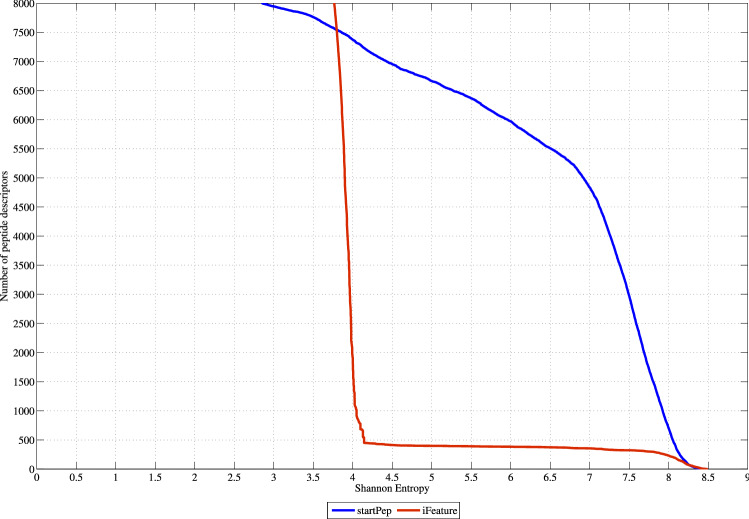
As a result of the VA, Fig. 2 depicts the SE distribution corresponding to the best 8000 ranked descriptors according to their SE values. As it can be noted, the starPep descriptors present better ability to discriminate among structurally different peptide sequences than the iFeature descriptors, since the formers have better SE distribution than the latter. The analyzed starPep descriptors present an average SE equal to 7.59 bits, whereas the iFeature descriptors have an average SE equal to 4.29 bits. More specifically, if we zoom in to the best 500 ranked descriptors, those from starPep always present SE values greater than 8 bits (83.77% of the maximum entropy), whereas only 231 iFeature descriptors are above the threshold aforementioned. In general, it can be concluded that the starPep descriptors have better information content than several types of peptide descriptor families. Thus, the starPep descriptors are useful for the mathematical characterization of a chemical space of BPs.
Figure 2.
Shannon’s entropy distribution for the iFeature descriptors versus starPep descriptors. This figure has been created using the R software package (version 3.5.1), available at https://cran.r-project.org/.
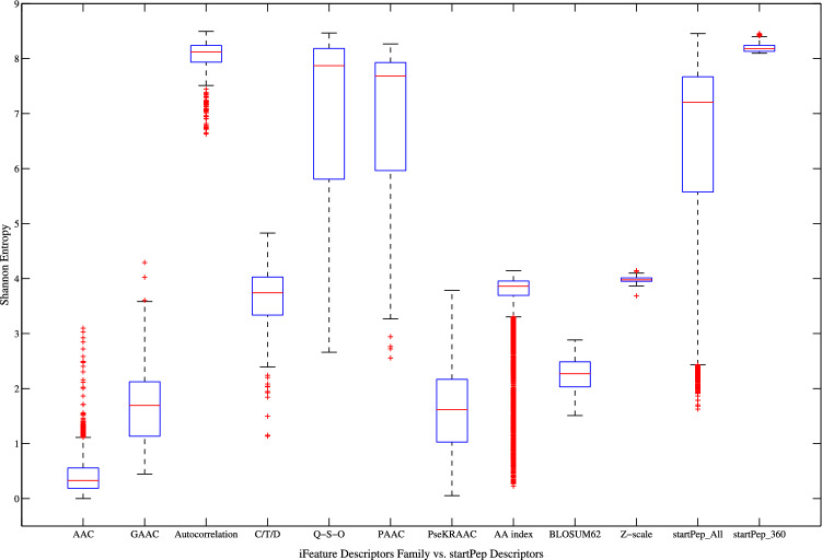
Moreover, Fig. 3 shows the boxplot graphics corresponding to each iFeature descriptor family (without removing correlated descriptors), as well as the corresponding ones to the starPep descriptors. It can be noted in this figure that the best iFeature descriptor families correspond to autocorrelation, Q-S-O, and PAAC indices, being the former the best of all. If these descriptor families are compared to the starPep descriptors (denoted as starPep_All), it can be observed that the 100 Q-S-O indices and 85 PAAC indices present a similar distribution regarding the 8416 starPep descriptors analyzed, whereas the 360 autocorrelation indices from iFeature present a better distribution. However, if the best 360 ranked descriptors from starPep are analyzed (denoted as starPep_360), then it can be observed that they present better distribution than the 360 autocorrelation indices from iFeature.
Figure 3.
Boxplots showing distributions of Shannon’s entropy for the iFeature descriptor families, as well as the starPep descriptors. This figure has been created using the R software package (version 3.5.1), available at https://cran.r-project.org/.
As a complement to the previous results, a linear independence analysis was performed by means of the PCA13 method. To this end, the iFeature and starPep descriptors with SE values greater than 8 bits were selected from the descriptor sets considered in the VA. Thereby, the input data for PCA is comprised of 700 starPep descriptors and 231 iFeature descriptors (SI1-6). By applying the PCA method on this feature space, orthogonal descriptors are strongly loaded (p-value ≥ 0.7) in different components, while collinear descriptors are loaded in the same component. Supplementary Information SI1-7 contains the eigenvalues and the percentages of the explained variance by the 11 principal components (PCs) obtained, which explain approximately 54.46% of the cumulative variance.
From the result table of PCA (SI1-7), we observed that some of the iFeature and starPep descriptors analyzed show collinearity in PC1 (16.64%) and PC4 (4.47%). For instance, in PC1, Q-S-O indices based on the Grantham chemical distance matrix26, for lag values from 1 to 13, are collinear with starPep descriptors encoding information related to amino acids favoring alpha-helix and uncharged polar amino acids, which were weighted with the third z-scale property. Moreover, in PC4, a single Q-S-O index based on the Schneider–Wrede physicochemical distance matrix27, for lag equals to 12, codified collinear information to starPep descriptors related to the isoelectric point and hydrophilicity amino acid properties. Additionally, the results obtained also indicate that the starPep descriptors have exclusive loads in the remaining components determined. That is, the iFeature descriptors studied did not present unique loadings in either of the components obtained.
Finally, three important conclusions can be drawn from the study so far: (1) the starPep descriptors seem to codify a degree of structural information captured by the iFeature descriptors, evidenced by the collinearity between the two groups; (2) there is structural information encoded by the starPep descriptors that is linearly independent to the iFeature descriptors; and (3) the iFeature descriptors seem not to codify different information respect to the starPep descriptors. These early outcomes demonstrate the applicability of the theoretical aspects of the starPep descriptors, and therefore, they should be useful in the construction of similarity networks.
Feature ranking and filtering
In this part of our experiments, we used starPep toolbox7 to initially compute 830 molecular descriptors on various datasets with different numbers of instances (n). For each dataset, the original descriptors and its corresponding reduced feature subsets were used as experimental data28 to assess the early stage of the feature selection process (Table 1). In this preliminary study, the calculated descriptors were ranked according to their entropy values, using the number of bins equal to n, and the entropy cutoff value () was set to 10% of maximum entropy (i.e., ) for removing irrelevant features from input datasets (Algorithm SI2-1). In general, there were at most 25 useless descriptors having information content less than the cutoff value, and they were removed.
Table 1.
Exploring the effect of changing the correlation method (Pearson’s or Spearman’s coefficient) and cutoff value () for assessing the similarity between subsets of candidate features and the original ones. Datasets and descriptors used in this experimental study are publicly available28.
| Datasetsa,b | Instances | Correlation threshold () | ||||
|---|---|---|---|---|---|---|
| Number of filtered descriptors (goodness-of-fit) | ||||||
| 0.5 | 0.6 | 0.7 | 0.8 | 0.9 | ||
| Pearson | ||||||
| Overall_NR98 | 32300 | 108 (0.36) | 156 (0.27) | 199 (0.22) | 275 (0.15) | 374 (0.09) |
| Overall_NR90 | 22512 | 111 (0.35) | 160 (0.27) | 208 (0.21) | 279 (0.15) | 372 (0.1) |
| Overall_NR70 | 14559 | 108 (0.37) | 150 (0.29) | 207 (0.21) | 276 (0.14) | 382 (0.08) |
| Overall_NR50 | 9428 | 108 (0.37) | 155 (0.28) | 198 (0.21) | 279 (0.14) | 378 (0.09) |
| Overall_NR30 | 4735 | 112 (0.37) | 155 (0.28) | 205 (0.19) | 281 (0.14) | 385 (0.08) |
| Antibacterial_NR98 | 10303 | 94 (0.35) | 147 (0.25) | 191 (0.19) | 282 (0.13) | 379 (0.09) |
| Antifungal_NR98 | 4546 | 101 (0.36) | 150 (0.26) | 202 (0.2) | 272 (0.14) | 380 (0.08) |
| Antiviral_NR98 | 3849 | 100 (0.37) | 143 (0.28) | 186 (0.21) | 280 (0.13) | 393 (0.08) |
| Anticancer_NR98 | 1557 | 98 (0.35) | 132 (0.28) | 188 (0.19) | 274 (0.12) | 395 (0.07) |
| Antiparasitic_NR98 | 501 | 111 (0.28) | 153 (0.21) | 211 (0.15) | 298 (0.1) | 402 (0.06) |
| Averages | 105 (0.35) | 150 (0.27) | 200 (0.2) | 280 (0.13) | 384 (0.08) | |
| Spearman | ||||||
| Overall_NR98 | 32300 | 94 (0.38) | 126 (0.3) | 177 (0.23) | 235 (0.18) | 338(0.09) |
| Overall_NR90 | 22512 | 95 (0.37) | 127 (0.31) | 174 (0.24) | 241 (0.18) | 327 (0.1) |
| Overall_NR70 | 14559 | 94 (0.38) | 127 (0.32) | 175 (0.25) | 235 (0.18) | 324 (0.1) |
| Overall_NR50 | 9428 | 95 (0.39) | 132 (0.31) | 174 (0.26) | 241 (0.18) | 327 (0.1) |
| Overall_NR30 | 4735 | 99 (0.37) | 134 (0.29) | 188 (0.22) | 241 (0.18) | 342 (0.1) |
| Antibacterial_NR98 | 10303 | 90 (0.35) | 121 (0.29) | 170 (0.22) | 232 (0.16) | 334 (0.1) |
| Antifungal_NR98 | 4546 | 87 (0.39) | 122 (0.29) | 177 (0.22) | 236 (0.16) | 338 (0.09) |
| Antiviral_NR98 | 3849 | 99 (0.35) | 133 (0.3) | 172 (0.22) | 241 (0.16) | 346 (0.09) |
| Anticancer_NR98 | 1557 | 92 (0.37) | 128 (0.27) | 172 (0.22) | 245 (0.14) | 352 (0.08) |
| Antiparasitic_NR98 | 501 | 94 (0.32) | 129 (0.24) | 179 (0.17) | 251 (0.12) | 361 (0.07) |
| Averages | 94 (0.37) | 128 (0.29) | 176 (0.23) | 240 (0.16) | 339 (0.09) | |
aThese datasets were retrieved from the database StarPepDB7.
bNR stands for Non-Redundant at a given percentage (number) of sequence identity. To carry out the sequence identity comparisons, we used a local alignment algorithm (Smith–Waterman30) implemented in BioJava31, with the BLOSUM62 substitution matrix.
After removing irrelevant features, all input datasets approximately kept 800 molecular descriptors sorted by their entropy values. Following that order, redundant features are removed, as described in Algorithm SI2-1. At this step, for the two correlation methods considered (Pearson’s or Spearman’s coefficient), several cutoff values were used to assess their effect at removing redundant variables (Table 1). Besides, Procrustes analysis29 was employed to check how much the complete set of descriptors can be reduced while preserving the data structure between the original and reduced descriptor space. On comparing the two descriptor spaces, the Procrustes goodness-of-fit is calculated between the first PCs of both the original and reduced sets of variables. The first 50 PCs were used since they explained at least 80% of the variance in the original data.
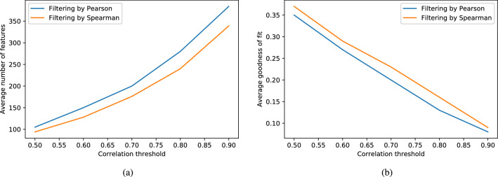
As can be seen in Table 1 and Fig. 4, the initial amount of calculated descriptors can be drastically reduced, providing some level of redundancy elimination in the resulting set of variables. As it is expected, decreasing the correlation threshold led to reducing the number of filtered features, being the Spearman coefficient, the one that least features retained. Moreover, looking at the Procrustes analysis, a low correlation threshold affects the goodness-of-fit between the original and reduced data. Whereas setting a high correlation threshold results in a better match between the reduced data structure and the original one, which is desired at this stage.
Figure 4.
Exploring the effect of changing the similarity threshold: (a) the average number of retained features is shown as an increasing function in similarity threshold; and, (b) the average goodness-of-fit between the 50 PCs of both the original and reduced features is shown as a decreasing function in similarity threshold. This figure has been created using the Python library Matplotlib (version 3.3.0), available at https://matplotlib.org/users/installing.html.
By analyzing Table 1, it can be noted that using Spearman and fixing the correlation threshold to 0.9 still yields a high number (> 300) of filtered descriptors; but a lower-number of descriptors (< 300) is retained when the correlation threshold is equal to 0.80, while the average goodness-of-fit is less than 0.2. It means that the resulting lower-dimensional space represents well enough the data structure of the original descriptor space. Thus, from now on, the Spearman correlation-based filter with a threshold equal to 0.8 will be the one used during the first stage of the feature selection process to compute a candidate set.
Feature subset optimization
So far, the resulting candidate set is still not enough lower-dimensional for the similarity network construction. Thus, the goal of the second stage is not the data structure preservation of the original descriptor space, but the optimization of a merit function (Eq. 7) to obtain an adequate feature subset. Table 2 shows the results for Algorithm SI2-2, where the best subset found for each dataset is characterized by the number of features and merit score. In general, the best-retained features are between 30 and 50, taking the square root of the number of instances as the number of bins (square-root choice32) for computing entropy and mutual information at this stage. Although there is no “correct” answer for the number of bins, the square-root choice led to good results in terms of the size of optimized subsets and merit scores, if compared with other alternatives (data not shown here).
Table 2.
Performance of feature subset optimization.
| Datasets | Instances (n) | Number of binsa () | Best subset found | CPU Timeb (hh:mm:ss) | |
|---|---|---|---|---|---|
| Number of features | Merit scores | ||||
| Overall_NR98 | 32300 | 179 | 39 | 3.985 | 12:07:03 |
| Overall_NR90 | 22512 | 150 | 40 | 3.87 | 05:17:40 |
| Overall_NR70 | 14559 | 120 | 42 | 3.667 | 01:27:46 |
| Overall_NR50 | 9428 | 97 | 39 | 3.474 | 00:34:04 |
| Overall_NR30 | 4735 | 68 | 33 | 3.13 | 00:08:12 |
| Antibacterial_NR98 | 10303 | 101 | 45 | 3.41 | 00:38:57 |
| Antifungal_NR98 | 4546 | 67 | 39 | 3.059 | 00:07:17 |
| Antiviral_NR98 | 3849 | 62 | 45 | 3.031 | 00:05:38 |
| Anticancer_NR98 | 1557 | 39 | 36 | 2.588 | 00:00:50 |
| Antiparasitic_NR98 | 501 | 22 | 40 | 2.11 | 00:00:05 |
aThe number of bins (data intervals) when constructing the histograms for computing the entropy and mutual information.
bThe feature subset optimization was performed in a Mac Pro Server with 2 x Intel Xeon Processor 2.66 GHz 6-cores, and memory 64 GB.
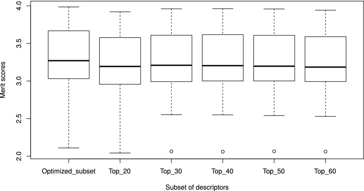
Additionally, Table 3 shows a comparison between the optimized subsets and the top-k ranked descriptors (with k between 20 and 60) from the full set of candidate features (without being optimized), according to their entropy values in descending order. For this comparison, a Pairwise Wilcoxon Rank Sum Test33 with Hochberg34 correction was used to evaluate differences among the selected groups of descriptors in Table 3. The statistical test revealed that the optimized subset is significantly better () than the top-k descriptors. Also, there are no significant differences between the top 30, top 40, and top 50 descriptors, which are likely to give the second-best scores. Furthermore, Fig. 5 summarizes the distribution of merit scores, and there can be observed atypical merit scores (outliers) for most groups of top-k descriptors. The presence of these outliers may suggest that the selection of those top-k descriptors may be affected by a small number of instances, such as the Antiparasitic_NR98 dataset (Table 3). Therefore, it can be concluded that the optimized descriptors (SI3-1) are suitable to characterize the chemical space of BPs.
Table 3.
Comparison among the best subsets found and top-k ranked descriptors.
| Datasets | Instances | Best merit scoresa | Merit scores of top-k ranked descriptorsb | ||||
|---|---|---|---|---|---|---|---|
| k | |||||||
| 20 | 30 | 40 | 50 | 60 | |||
| Overall_NR98 | 32300 | 3.985 | 3.92 | 3.96 | 3.962 | 3.958 | 3.942 |
| Overall_NR90 | 22512 | 3.87 | 3.79 | 3.827 | 3.829 | 3.822 | 3.807 |
| Overall_NR70 | 14559 | 3.667 | 3.577 | 3.608 | 3.616 | 3.607 | 3.589 |
| Overall_NR50 | 9428 | 3.474 | 3.368 | 3.396 | 3.406 | 3.403 | 3.388 |
| Overall_NR30 | 4735 | 3.13 | 3.051 | 3.057 | 3.044 | 3.038 | 3.035 |
| Antibacterial_NR98 | 10303 | 3.41 | 3.336 | 3.361 | 3.364 | 3.356 | 3.334 |
| Antifungal_NR98 | 4546 | 3.059 | 2.98 | 3.018 | 3.01 | 3.011 | 2.993 |
| Antiviral_NR98 | 3849 | 3.031 | 2.956 | 2.992 | 3.001 | 3.001 | 2.995 |
| Anticancer_NR98 | 1557 | 2.588 | 2.517 | 2.552 | 2.55 | 2.54 | 2.529 |
| Antiparasitic_NR98 | 501 | 2.11 | 2.042 | 2.063 | 2.06 | 2.065 | 2.061 |
| Averages | 3.232 | 3.154 | 3.183 | 3.184 | 3.180 | 3.167 | |
aMerit scores of best subsets found.
bMerit scores of the top-k ranked descriptors from the candidate feature set.
Figure 5.
Box plot of merit scores. This figure has been created using the R software package (version 3.5.1), available at https://cran.r-project.org/.
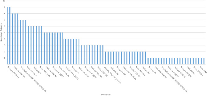
To illustrate that the optimized descriptors adequately characterize a particular chemical space, we have accounted for the number of distinct datasets that include a selected descriptor. The results are presented in Fig. 6. The x-axis lists descriptors sorted by the most common ones in all datasets. The y-axis represents the number of datasets that include the specified descriptors. It can be noted that there are just three descriptors repeated in nine out of the ten datasets. Besides, the trend in the chart indicates that the majority of descriptors reappear only in a few databases. Indeed, many of them appear solely in a single dataset.
Figure 6.
Number of distinct datasets that include a selected descriptor. This figure has been created in Excel 2016, available at https://www.microsoft.com/es-mx/software-download/office.
Generating molecular similarity networks
According to the above results, we used the optimized descriptors (SI3-1) to built molecular similarity networks based on (i) the traditional CSNs14–16, or (ii) the sparse HSPNs35. Note that whereas the fully connected CSN at threshold is prohibitive for large datasets, an alternative connected network may be successfully generated based on HSPNs (Algorithm SI2-3). The feasibility of building such HSPNs from the experimental datasets is illustrated in Table 4. It can be observed that the generated HSPNs achieve low-density levels in all cases, including large datasets.
Table 4.
Summary for the alternative HSPNs generated at threshold .
| Datasets | Nodes | Max | Similarity relationshipsb | |
|---|---|---|---|---|
| distancea | Edges | Network density | ||
| Overall_NR98 | 32300 | 29.80 | 353 213 | 6.8E-4 |
| Overall_NR90 | 22512 | 27.22 | 242 227 | 9.6E-4 |
| Overall_NR70 | 14559 | 27.03 | 157 590 | 0.001 |
| Overall_NR50 | 9428 | 27.01 | 102 226 | 0.002 |
| Overall_NR30 | 4735 | 23.65 | 46338 | 0.004 |
| Antibacterial_NR98 | 10303 | 27.95 | 95605 | 0.002 |
| Antifungal_NR98 | 4546 | 24.00 | 36765 | 0.004 |
| Antiviral_NR98 | 3849 | 24.12 | 31709 | 0.004 |
| Anticancer_NR98 | 1557 | 21.56 | 9552 | 0.008 |
| Antiparasitic_NR98 | 501 | 19.13 | 2560 | 0.02 |
aThe maximum distance between two points in the defined descriptors space.
bSimilarity relationships at . The HSPN at is a connected subnetwork having a low-density level in all datasets.
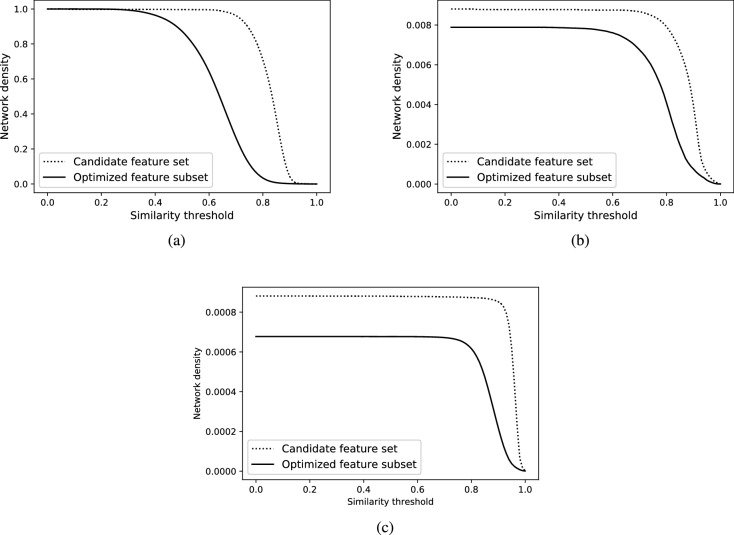
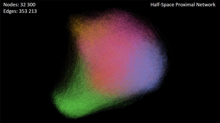
Furthermore, the impact of optimized descriptors can also be seen in the construction of the molecular similarity networks, either CSNs or HSPNs. As depicted in Fig. 7, by interpreting the performance of descriptors as a function of network density, the optimized feature subset yields lower density levels with a smoother appearance than the density curves of the complete candidate feature set. This shows that, even for large datasets such as Overall_NR98 (Fig. 7c), the optimized descriptors are suitable for generating a lower-density similarity network to be analyzed by visual inspection (Fig. 8).
Figure 7.
Examining the impact of using the optimized feature subset versus the full set of candidate features for similarity network construction. Density curves were generated at varying the similarity threshold in the following networks: (a) CSNs from Anticancer_NR98, (b) HSPNs from Anticancer_NR98, and (c) HSPNs from Overall_NR98. In contrast to CSNs, the natural density of HSPNs is low at any threshold, even for . This figure has been created using Python Matplotlib (version 3.3.0), available at https://matplotlib.org/users/installing.html.
Figure 8.
Visualizing the similarity network (HSPN) of a vast set of BPs (Overall_NR98) at threshold , using the ForceAtlas2 layout algorithm36. This figure has been created using the software starPep toolbox (version 0.8), available at http://mobiosd-hub.com/starpep/, and PowerPoint 2016 available at https://www.microsoft.com/es-mx/software-download/office.
Visual analysis of chemical space
Visualization and interactive exploration of the generated similarity networks may serve to form a visual image into the mind aimed at facilitating analytical reasoning not possible before. However, understanding networks through visual inspection is not a straightforward process37, and thus we propose a systematic network exploration using a combination of clustering and network science techniques. During this exploration process, three aspects of visual inspection are useful for aiding human thinking: positioning, filtering, and customizing the appearance of nodes7.
To facilitate the above-mentioned network analysis, the proposed workflow in Fig. 1 has been implemented in the software starPep toolbox (http://mobiosd-hub.com/starpep/), allowing end-user to generate and navigate similarity networks by their own needs and interests. On this basis, as described next, we illustrate the use of the proposed workflow to carry out three case studies for finding and analyzing relevant nodes in molecular similarity networks of BPs.
Case study I: navigating a biologically relevant chemical space
The 1557 anticancer peptides (Anticancer_NR98) to be analyzed here are given in SI4-1 (FASTA file). Also, for each peptide discovered to be a relevant node, additional information (metadata7) is available in SI4-2 (Excel file). As the dataset Anticancer_NR98 is not large enough, we generate traditional similarity networks (CSNs) from the similarity/distance matrix calculation. To visualize these similarity networks in a meaningful way, we examine a family of force-directed layout algorithms that can be used to spatialize the network and rearrange nodes38. These algorithms change the position of nodes by considering that they repulse each other, whereas similarity relationships may attract their attached nodes like springs. Particularly, the Fruchterman-Reingold algorithm39 was the most suitable for drawing the network of anticancer dataset (Fig. 9).
Figure 9.
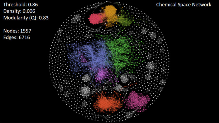
Visualizing the CSN of anticancer peptides (Anticancer_NR98) at similarity threshold of 0.86, using the Fruchterman-Reingold layout algorithm39. Nodes are colored according to the leading communities to which they belong. This figure has been created using the software starPep toolbox (version 0.8), available at http://mobiosd-hub.com/starpep/ , and PowerPoint 2016 available at https://www.microsoft.com/es-mx/software-download/office.
Exploring and mining community structures. A CSN having an arbitrary low density () can be visualized at first sight by setting a large threshold (Fig. 7a). Also, networks become more interpretable through visual inspection if having a community structure40. Note that communities of BPs may represent some biologically relevant regions of chemical space where bioactive compounds reside9. Hence, we have explored the CSNs by varying the similarity threshold until a well-defined community structure emerged. In this way, a final CSN has been analyzed by adjusting the similarity threshold to 0.86, at network density of 0.006, achieving network modularity (Q) of 0.83 (Fig. 9).
Based on our visual exploration, we corroborate what other authors have previously remarked41; there is higher network modularity at large similarity threshold. Nonetheless, the interval within which the threshold value should be explored is not fixed, and it depends on the input dataset. We also suggest that the final decision for picking a high threshold value should be made carefully to avoid an edgeless network structure (Fig. 7).
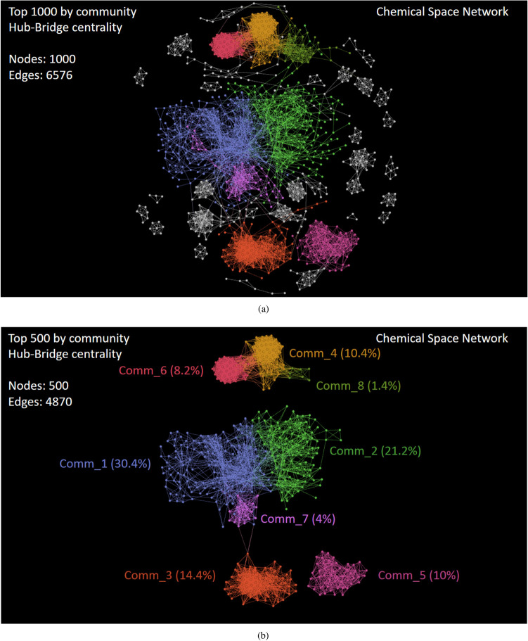
Local centrality analysis. Once a community structure is found, we rank nodes in decreasing order according to the community Hub-Bridge centrality measure (Eq. 13) for retaining the top-k of the ranked list. Particularly, the top 1000 exposes densely connected groups of nodes like cliques, which are defined to be complete subgraphs (Fig. 10a). These related sequences may be forming families in the chemical space of anticancer peptides, and detecting them may be of use in future works42,43.
Figure 10.
Visualizing the subnetwork of anticancer peptides having the (a) Top 1000 and (b) Top 500 ranked nodes by the Community Hub-Bridge centrality. This figure has been created using the software starPep toolbox (version 0.8), available at http://mobiosd-hub.com/starpep/, and PowerPoint 2016 available at https://www.microsoft.com/es-mx/software-download/office.
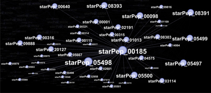
Of course, nodes inside large communities have higher centrality value and better ranking than those inside smaller groups. Then, we select the top 500 as the representative ones of eight leading communities (Fig. 10b). These local central peptides inside each leading community are given in SI4-3 (FASTA files), and they may be representing sequence fragments or naturally occurring peptides that could be identified as starting points for lead discovery1,20. For instance, the peptide starpep_00185 (known as ascaphin-844) is the most central node inside Community 1 (Fig. 11), and some of its peptide neighbors are analogs containing aminoacids substitutions (Table 5). When looking for additional information about this peptide (SI4-2), we noticed that ascaphin-8 is the naturally occurring one, while chemically modified peptide analogs may have greater therapeutic potential45,46.
Figure 11.
A zoom into the Community 1 for highlighting the most central node (starPep_00185) based on the Hub-Bridge centrality. Nodes are resized according to their local centrality measures. This figure has been created using the software starPep toolbox (version 0.8), available at http://mobiosd-hub.com/starpep/, and PowerPoint 2016 available at https://www.microsoft.com/es-mx/software-download/office.
Table 5.
A family of central peptides inside community 1.
| IDa | Sequenceb | Length |
|---|---|---|
| starPep_00185 | GFKDLLKGAAKALVKTVLF | 19 |
| starPep_05498 | GFKDLLKGAAKALVKAVLF | 19 |
| starPep_05497 | GFKDLLKGAAKALKKTVLF | 19 |
| starPep_05500 | GFKDLLKGAKKALVKTVLF | 19 |
| starPep_03114 | GFKKLLKGAAKALVKTVLF | 19 |
| starPep_05499 | GFKDLLKGAAKALVKTVKF | 19 |
aID of the peptides in starPepDB7.
bAdditional information can be found in SI4-2.
Ascaphin-8 is a 19-mer peptide containing a C-terminally α-amidated residue (GFKDLLKGAAKALVKTVLF.NH2). It is one out of eight structurally related antimicrobial peptides, termed ascaphin 1-8, that were originally isolated from the skin secretions of the tailed frog Ascaphus truei44. Among the eight purified peptides, ascaphin-8 was the most active compound against a range of pathogenic microorganisms, but it also had limited therapeutic potential due to the greatest hemolytic activity44. However, its lysine-substituted analogs showed very low hemolytic activity while displaying potent antibacterial activity against a range of clinical isolates of extended-spectrum β-lactamase producing bacteria46. In addition to the broad-spectrum antimicrobial activity, the anticancer property of ascaphin-8 and its analogs has been tested on human hepatoma-derived cells (HepG2), where analogs showed enhanced cytotoxicity to the HepG2 cells and reduced toxicities against mammalian cells when compared with ascaphin-845. Furthermore, other studies47–49 revealed that ascaphin-8 may be considered as a starting point for Lead Discovery.
Case study II: finding central but non-redundant peptides
As can be observed in Table 5, some neighbor nodes in the interior of communities may be representing a family of similar peptides. Another example of closely related structures can be seen in all 50 members of the Community 5 (see Comm_5 in Fig.10b). The peptides inside this community have the same sequence length of 10 aa. Also, the same amino acid residues compose those 50 peptides, with two amino acids fixed at positions 6 and 10 (see SI4-3 for more sequence details). Therefore, in general, it is expected that there are many nodes with similar centrality values in the network, and it may be better to extract some non-redundant nodes from communities than just selecting the highest-ranked ones.
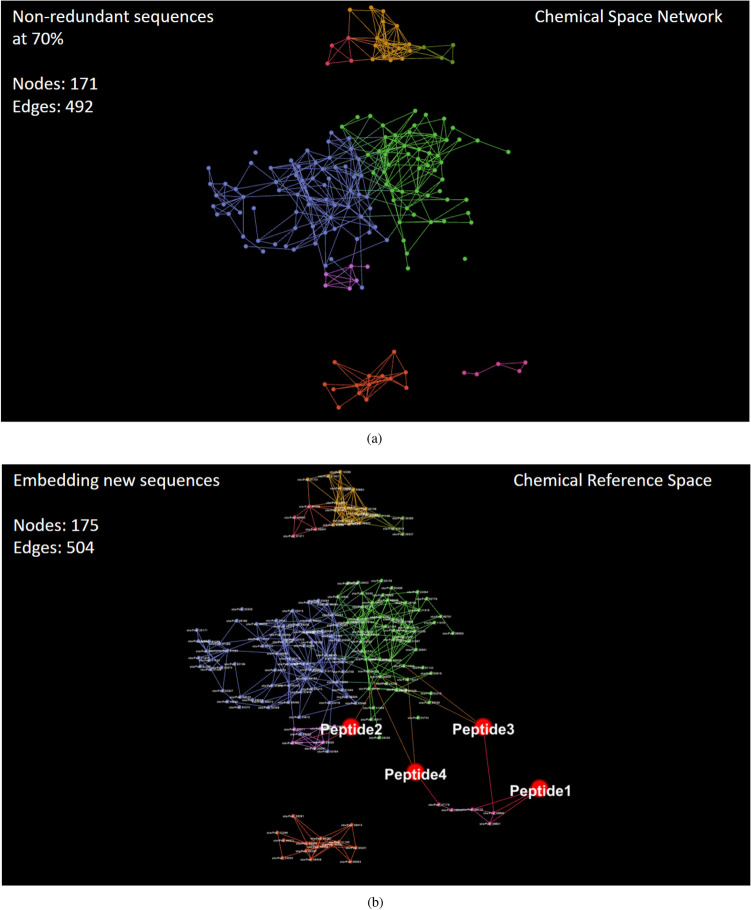
Next, to clearly extract central but non-redundant peptides from each community in Fig. 10b, we first sort nodes according to the decreasing order of their local centrality values. Following that order, the redundant sequences are removed at a given percentage of sequence identity. The resulting subnetwork is presented in Fig. 12a. We have used 70% of sequence identity to consider that a particular sequence is related to an already selected central peptide and, as a consequence, removed from the network. For these sequence comparisons, we also applied the Smith–Waterman algorithm30 implemented in BioJava31, with the BLOSUM62 substitution matrix. Finally, we ranked the non-redundant peptides according to their decreasing values of Harmonic centrality measure (Eq. 12). The sorted list is given in SI4-4 (FASTA file), and the topmost ranked peptides are those having relatively small similarity paths to all other nodes in the network.
Figure 12.
Visualizing the (a) subnetwork of anticancer peptides having central but non-redundant structures at 70% of sequence identity, and (b) the projection into this network of four in-silico designed anticancer peptides (Peptide1–4)50. This figure has been created using the software starPep toolbox (version 0.8), available at http://mobiosd-hub.com/starpep/, and PowerPoint 2016 available at https://www.microsoft.com/es-mx/software-download/office.
Case study III: embedding new sequences into a network model
Projecting new sequences into similarity networks of known bioactive peptides may serve to identify the region in a chemical reference space where the new compounds reside. Firstly, the currently selected descriptors are computed for the new peptides to be inserted. Then, each projected peptide is connected to its k nearest neighbors in the defined metric space for further analysis. To illustrate this process, we have embedded four in-silico designed anticancer peptides50 in the molecular similarity network under study: Peptide1 (WLFKFLAWKKK), Peptide2 (FPKLLLKFLRLG), Peptide3 (KKFALKLFWWK), and Peptide4 (RLLRRLRIRG).
As can be seen in Fig. 12b, Peptide1, and Peptide2 are occupying different positions in a chemical reference space of anticancer peptides. According to Ref.50, these two experimentally verified peptides were the most active peptides, and molecular dynamics simulations suggest that they have different interaction mechanisms with heterogenous POPC/POPS lipid bilayer membranes. Whereas the Peptide1 remains adsorbed to the membrane surface, the Peptide2 has membrane penetration capability50.
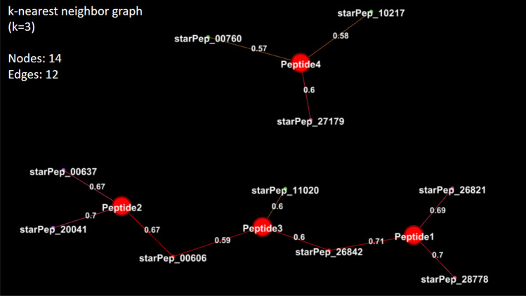
Furthermore, Fig. 13 reveals the K-Nearest Neighbor Graph (K-NNG), with , based on the Euclidean distances in the defined descriptor space. It can be observed that Peptide3, which is an active compound too, is lying on a similarity path between Peptide1 and Peptide2. Indeed, Peptide3 is more similar to Peptide1 by the length of their similarity path, and less similar to Peptide2, which is expected since Peptide3 and Peptide1 are analogs of the same peptide50. However, despite Peptide2 and Peptide4 are having a common origin, Peptide4 is inactive50, and it is not connected to the previous ones in the K-NNG. Therefore, this retrospective analysis points out that the approach presented here may be useful for getting insight into the chemical space of BPs.
Figure 13.
Visualizing the K-Nearest Neighbor Graph () of the new compounds of interest (Peptide1–4)50 and the recovered peptides (neighbor nodes) from a chemical reference space. Additional information for the recovered peptides can be found in SI4-2. This figure has been created using the software starPep toolbox (version 0.8), available at http://mobiosd-hub.com/starpep/, and PowerPoint 2016 available at https://www.microsoft.com/es-mx/software-download/office.
Conclusion
Here, we have designed and implemented a workflow that transforms automatically raw data of amino acid sequences into a meaningful graph-based representation of chemical space, such as a molecular similarity network. The proposed workflow takes peptide sequences as input to project all these n compounds into an m-dimensional descriptor space, where both n and m are natural numbers with . To project each peptide sequence, we calculate molecular descriptors by applying statistical and aggregation operators on amino acid property vectors. Then, using the concepts of entropy and mutual information, an optimized subset of the original features is automatically selected for removing the irrelevant and redundant ones. This allows reducing dimensionality to avoid dealing with high-density networks and increasing efficiency in the definition of descriptor space. We also have conducted experiments for learning and tuning the fully automatic construction of similarity networks from raw data of known bioactive peptides. Our experimental results showed the efficacy of our approach for supporting visual graph mining of the chemical space occupied by a comprehensive collection of bioactive peptides. To illustrate this mining task, we applied a systematic procedure based on network centrality analysis for navigating and mining a biologically relevant chemical space known to date. Therefore, we hope to encourage researchers to use our approach for turning bioactive peptide data into similarity networks into information that could be used in future studies.
Methods
This section firstly describes how to define a multi-dimensional descriptor space from the amino acid sequences of BPs, which involves molecular descriptors calculation and unsupervised feature selection method. The second part of the section is about how to generate a similarity network from the defined descriptor space, and consequently, how to understand the generated networks through clustering and network science techniques40.
Defining a multi-dimensional descriptor space
The molecular features to be calculated from the peptide sequences may account for physicochemical properties and information about structural fragments or molecular topology51. To this end, we extend our in-house Java library7 to compute hundreds or thousands of proposed MDs (Tables SI1-1 and SI1-2). The MDs described in Table SI1-1 are legacy descriptors accounting for physicochemical properties, and they were formerly implemented by reusing free software packages to carry out previous studies52,53. Unlike the legacy descriptors, new descriptors (those in Table SI1-2) are implemented by applying statistical and aggregation operators on amino acid property vectors, e.g., measures of central tendency, statistical dispersion, OWA operators54,55, and fuzzy Choquet integral operators56,57. Further, it should be noted that the reasons for using these operators in the calculation of MDs have been demonstrated elsewhere58–62.
Let be a descriptor matrix whose rows and columns represent peptide instances and calculated features, respectively, i.e., encodes the numerical value for the jth descriptor of the ith peptide sequence. Then, denoting the feature j as , which is the jth column of matrix , an optimization method for feature selection is aiming to identify the best subset of features among all possible subsets. Nonetheless, finding the optimal subset is a hard goal to achieve since the assessment of all possible subsets is not feasible (there are subsets, where m is the number of original features), and no efficient algorithm is known that solves this problem. Accordingly, to be able to formulate and solve an optimization problem for subset selection, we first need to introduce some basic definitions for analyzing the relevance and redundancy of features.
Basic definitions
Shannon’s entropy63. Entropy can be considered as one criterion for measuring relevance in the field of unsupervised feature selection64,65. A particular calculation of entropy has been proposed in Ref.23 to capture the information content of descriptor distributions represented in histograms. For instance, Fig. 14 shows the histograms generated for two molecular descriptors and their information contents. The histograms were constructed by dividing the data range of each variable into the same number of data intervals (bins). Using this binning scheme is possible to transform continuous features into discrete variables that count the number of feature values per bins. Note that the definition of entropy for continuous variables is hard to compute66. On this basis, a discretization mechanism can be applied to compute the entropy measure as follows.
Figure 14.
Shannon entropy calculated for two molecular descriptors using the bining scheme of histograms. (a) Shannon entropy (H) = 0.068; and, (b) Shannon entropy (H) = 2.21. This figure has been created using the R software package (version 3.5.1), available at https://cran.r-project.org/.
Suppose that for each feature, its range is divided into the same number of bins . Then, new data representation is generated looking at the peptides that adopt a value located at bin i for each feature. Let be the set of peptides whose value fall in the bin i for feature j, the frequentist probability of finding a value within a specific data range i for feature j is calculated by dividing the data count by the summed count of all bins:
| 1 |
This frequentist probability is used to compute the entropy H of feature j:
| 2 |
As an upper bound, the maximum entropy is reached when all data intervals are equally populated, i.e., each bin is occupied by the same amount of peptides. By contrast, the minimum entropy () is reached if all feature values fall within a single bin i. In general, broad histograms result in higher entropy values than narrow histograms, as can be seen in Fig. 14. Therefore, a descriptor with high entropy near to the maximum value means uniform distribution of feature values and should be retained. Conversely, a descriptor with low entropy near to the minimum value is having low information content and should be removed.
Mutual information66. Considering two discrete random variables X and Y with a joint probability p(x, y), the mutual information I(X, Y) is a measure of the dependency between them, and can be used as redundancy criterion between two molecular descriptors (Fig. 15)67. Let be the intersection set containing those peptides whose values fall in the bins i and l, for features j and k, respectively. The joint probability of observing at the same time two values falling in the bin i and l is estimated as:
| 3 |
Figure 15.
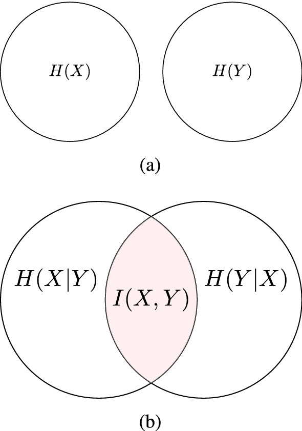
This figure depicts the relationship between entropy and mutual information for two variables X and Y. I(X, Y) measures the amount of information content that one variable contains about another. (a) I(X, Y) is equal to zero if and only if X and Y are statistically independent; and, (b) , which corresponds to the reduction in the entropy of one variable due to the knowledge of the other. Hence, the I(X, Y) can take values in the interval: ; the larger the value of I(X, Y) is, the more the two variables are related. This figure has been created using the package TikZ (version 0.9f 2018-11-19) in Latex, available at https://www.ctan.org/pkg/tikz-cd.
Then, using the marginal and joint probabilities defined in Eqs. 1 and 3, respectively, we computed the mutual information between two features:
| 4 |
In addition to the mutual information criterion, a correlation coefficient is another measure for assessing the redundancy between variables68.
Correlation-based measures69. Pearson correlation coefficient () is a well-known criterion for measuring the linear association of a pair of variables X and Y69. This correlation coefficient as a criterion of redundancy between two features is given by
| 5 |
where and indicate, respectively, the ith value and the mean of the feature . We used the absolute value since the sign of the coefficient only indicates that, in case of positive sign, both feature values tend to increase together or, in case of negative sign, the values of one feature increase as the values of the other feature decrease. If two features have an exact linear dependency relationship, is 1; if two features are totally independent, is 0; whereas larger values in the range [0, 1] indicate higher linear correlation. However, this correlation coefficient is not suitable to capture the dependency between two variables that is not linear in nature.
In addition to the Pearson correlation coefficient, Spearman’s rank correlation coefficient () measures the monotonic relationship (whether linear or not) for a pair of variables X and Y69. This correlation coefficient relies on the rank order of values for each variable instead of the value itself, i.e., it assesses the similarity between the two rankings rank(X) and rank(Y) rather than comparing raw values of X and Y, where rank() denotes the data transformation in which original values are replaced by their position when the data are sorted. The formula for Spearman’s coefficient is based on Pearson’s correlation () with the distinction of being computed on ranks:
| 6 |
We also used the absolute value of the monotonic correlation coefficient as a criterion of similarity between two features. If one feature is a perfect monotone function of another, then is 1; if they are totally uncorrelated, is 0; otherwise, lies in the range [0,1] and it is high when the values of two features have a rank correlation, and low when values have a dissimilar rank.
Unsupervised feature selection
Here we present a two-stage procedure for solving a feature subset selection problem. In the first stage, a candidate feature subset is selected by removing irrelevant and redundant features from the original set (Algorithm SI2-1). At this stage, descriptors are ranked in descending order of their entropy values to choose the top-ranked ones or those having entropy values greater than a given threshold. In this way, relevant features are progressively selected as long as they are not correlated to any of the already selected ones. Moreover, an assessment helped to decide whether two features are correlated or not, since either Pearson’s or Spearman’s coefficient may be used with different correlation thresholds.
The effect of changing both the correlation method and cutoff value was analyzed in an experimental study. We used a Procrustes analysis29 to quantitatively assess the quality of retained features in the candidate subset for representing the original ones70,71. This analysis consists of measuring proximities between the original and reduced descriptor spaces describing the same set of peptides. So the optimal transformation should be applied to one feature space based on scaling, rotations, and reflections, to minimize the sum of squared errors as a measure of fit (goodness-of-fit criterion). Since the original feature space and the reduced space are having different dimensions, they can be properly comparable by using the same amount of principal components13. Therefore, the goodness-of-fit criterion equals to 0 may indicate that the two descriptor spaces coincide. On the contrary, a goodness-of-fit value equals to 1 means that the two descriptor spaces are utterly dissimilar.
In the second stage, the aim is to find the best subset containing the most informative and less redundant features from the candidate set. Indeed, the number of previously selected features can be further reduced by finding a solution to an optimization problem. We define the problem to solve as
| 7 |
where is the objective function, and F is a subset of features over the search space of all possible subsets from the candidate feature set. By looking more deeply into the objective function, one can see that is defined as a subtraction between the average of entropy values and the average of normalized mutual information as a penalization term. Maximizing this subtraction expression is a simple form of maximizing the first term as a measure of relevance, while minimizing the second term as a measure of redundancy67.
Our definition of is based on a previous work67, where the class label information is available. In our case of unsupervised feature selection, no class labels are available. Thus, we modify the previous definition in Ref.67 to satisfy our needs. Additionally, we have incorporated the ranking and filtering stage for an early removing of irrelevant and redundant features. In that early stage, both the features with low entropy values affecting the average in the first term of , and those with high redundancy in the second term of the subtraction are removed.
Despite an early removal of useless and correlated features, an exhaustive search over all possible subsets of the candidate feature set is computationally unaffordable. Thus, it is possible to use a heuristic search strategy that may give good results, although there is not guarantee of finding the optimal subset. We adopt a greedy hill-climbing procedure (Algorithm SI2-2) that starts with the full set of candidate features and eliminates them progressively (backward elimination64). This procedure traverses the search space by considering all possible single feature deletions at a given set, and picking the subset with the highest evaluation according to the objective function .
Translating a descriptor space into similarity networks
After calculating and selecting MDs, the workflow stage is the translation of the molecular descriptor space into similarity networks. Assuming no distinction between a node and the peptide it represents, the similarity network is constituted by a set of nodes that are characterized by feature vectors (descriptors) in a metric space. Then, the Euclidean distance d(u, v) between two nodes u, v can be transformed into a pairwise similarity measure by using the following formula:
| 8 |
As it was suggested in Ref.41, the definition of sim(u, v) is suitable to construct a similarity network: there is an edge between nodes u and v if their pairwise similarity value is equal or greater than a given threshold t, i.e., if . In our case, we considered these networks as weighted graphs. That is, for a given threshold t the similarity matrix that stores the similarity values () of every pair of peptides becomes an adjacency matrix whose values are given by
| 9 |
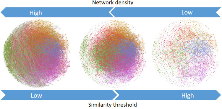
Keeping in mind that the perception of similarity is in the eyes of the beholder72, we considered that the threshold is a user-defined parameter to be explored. Besides, a predefined constant value for t is not useful in practice because the distribution of similarity values may strongly vary depending on the input dataset. Note that when the threshold t is modified, the number of edges might change, whereas the number of nodes remains unchanged. Thus, some network properties can be altered as a function of the parameter t, e.g., network density (Fig. 16).
Figure 16.
Network density at varying similarity thresholds. This figure has been created using the software starPep toolbox (version 0.8), available at http://mobiosd-hub.com/starpep/, and PowerPoint 2016 available at https://www.microsoft.com/es-mx/software-download/office.
Network density is defined as the ratio between the number of edges and the total number of possible relationships:
| 10 |
where , and . In the extreme case where threshold , all compounds are considered similar, and the complete network with edges would be drawn (). On the contrary, when , a minimally connected network is realized (). In general, when t increases the network density tends to decrease (Fig. 16).
Of course, the task of understanding what networks are telling us depends on a chosen value of t. It may become more complicated at low threshold values yielding densely connected nodes, since a picture with too many lines will be difficult for human eye perception. Networks cannot be readily interpretable at high levels of their density values. Moreover, large networks with thousands of nodes and millions of possible relationships may require high memory usage. It may cause out of memory errors when computing and loading the graph into the RAM of personal computers.
A straightforward way of achieving low levels of density is using a high value of threshold t (Fig. 16). At large values of t, the similarity networks can be readily interpretable41. Nonetheless, increasing too much this value may give rise to edgeless networks, either disconnecting many nodes or isolating groups of them. Therefore, the parameter t should be handled carefully to achieve interpretable graphs without losing information from the network topology. Setting an inappropriate value for the threshold t may be yielding networks where the topological information is hidden15.
Half-space proximal networks
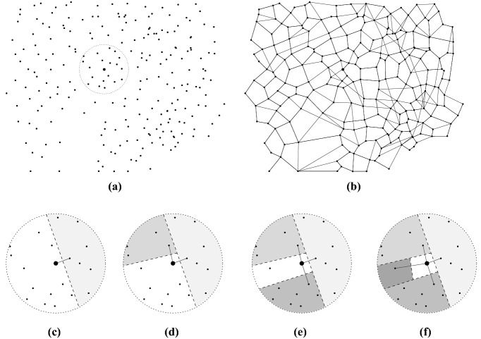
When constructing a similarity network for a large dataset of BPs (ten of thousands of them), the amount of RAM required is very high to store the matrix to be pruned. Hence, what is needed here is the creation of a sparse network with similarity/distance properties near to that of the complete graph, but where only a small fraction of the possible maximum number of links among nodes are used. One such network is achieved by the Half-Space Proximal (HSP) test35, which is a simple algorithm that may be applied to build similarity networks with lower-density levels than CSNs. The HSP test extracts a connected network over a set of points in a metric space, in our case, the multi-dimensional descriptor space, and it works as follows.
Assuming for simplicity a two-dimensional (2D) space, Fig. 17 illustrates how the HSP test is applied to an arbitrary set of points. For an initial point u, its nearest neighbor v is taken to add an edge between them. Then, the 2D space is divided into two half-planes by an imaginary perpendicular line passing through the midpoint of the edge connecting u and v. Notice in Fig. 17 that one half-plane is the region of points (the shaded ones) closer to v than to u, and this region is called the forbidden area for the point u. Next, from the remaining candidate points that do not belong to the forbidden area, the nearest point is taken to be the new neighbor of u. These steps are repeated until the candidate set of points is empty.
Figure 17.
Applying the HSP test for extracting neighbors of a given point: (a) Initial configuration; (b) Final configuration; (c) 1st neighbor; (d) 2nd neighbor; (e) 3rd neighbor; and, (f) 4th neighbor. The above image is a modified version of Fig. 1 in Ref.35. This figure has been created using the software IPE (version 7.2.20), available at http://ipe.otfried.org/.
The procedure described above can be independently applied to each point in the metric space. Thus, we made a parallel implementation of the HSP test (Algorithm SI2-3). The resulting relationships between nodes and their HSP neighbors comprise the HSP network called in short as HSPNs. These HSPNs are subgraphs of the CSNs, denoted by , where for an arbitrary threshold t. We also consider as a weighted network, where the weight function is indicating the similarity values (Eq. 8) of connected peptides.
Understanding the generated similarity networks
So far, we have emphasized on how to build a molecular descriptor space and meaningful network representations describing similarity relationships between peptides. Now, we will suggest how network science techniques can be used to get a deeper insight into the generated similarity networks. In practice, we implement some functionalities based on the open source project Gephi73. The main idea we pursue is that researchers may perceive the graph structure and seek nodes occupying important roles within a network of interest.
Detecting communities
Clustering is a fundamental technique in unsupervised learning for finding and understanding the hidden structure in the data. This technique consists of separating data elements into several groups, such that elements in the same group are similar and elements in different groups are dissimilar to each other. The resulting groups are called clusters or communities in the case of networks40. As such, the usage of clustering to identify densely connected nodes has been known as community detection74, and the detected communities may represent various groups of compounds having different chemical properties in the context of a molecular similarity network.
One effective approach for network community detection has been to maximize a quality function called modularity75, which is useful for evaluating the goodness of a partition into communities. This modularity measure is the fraction of edges connecting nodes in the same community minus the expected value of the same quantity in a network with identical community structure and degrees of vertices, but where edges are placed randomly. Formally, modularity (Q) for a weighted network has been defined as76:
| 11 |
where is the weight of the edge (in our case the similarity value) between nodes i and j or 0 if there is no such connection, is the total sum of weights in the whole network, is the sum of weights of the edges attached to node i, is the community to which node i is assigned, and is 1 if both vertex i and j are members of the same community () or 0 otherwise.
The modularity Q (Eq. 11) can be either positive or negative, and its maximum value is 175. For maximizing Q over possible network divisions, we used the Louvain Clustering algorithm77 implemented in Gephi. This algorithm has achieved good results in terms of accuracy and computing time if compared with other available methods in the literature77,78. It initially assigns a different community to each node of the network. Then, for each node u, it evaluates the gain of modularity that would take place by moving node u to the community of its neighbors. The movement of placing node u in the community of node v is done if the gain achieves the highest positive contribution to the modularity. If no positive gain contribution is achieved, the node u stays in its original community. This first phase is repeated for all nodes until no further improvement is possible. Later, in a second phase, the algorithm builds a new network whose nodes are the communities found in the previous phase. Once again, the first phase is reapplied to the new network and stops when there is not a movement that can improve the modularity.
Ranking nodes based on centrality measures
Centrality is a concept that has been widely used in another field of sciences, such as social network analysis, to identify influential nodes in a network under study40,79,80. Formally, a centrality measure C(u) is a function that assigns a non-negative real number to each node u in the network40. Then, a basic analytic task lies in finding those nodes that are more likely to be of interest for drug discovery according to the values of C(u)20. To this end, one may focus on quantifying either a global or local measure of how important a node is in a given network80.
Global centrality measures consider the whole network, and of course, they are more costly to compute than local measures using only neighborhood information80. For instance, Harmonic Centrality81 is one distance-based centrality measure deemed to be global. This centrality for a node i is defined as
| 12 |
where the geodesic distance is the length of the shortest path from i to j. At considering that the shortest path length is calculated using Dijkstra’s algorithm, by convention, and if there is no such path when dealing with unreachable nodes in disconnected networks. That means that the worst-case complexity is quadratic in the number of nodes, which may be inefficient for many large networks82.
In contrast to global measures, local centrality measures are only based on information around nodes80, and they are shown to be useful by exploiting the community structure. Indeed, it is reasonable to find network communities to identify which are the most influential nodes by analyzing the detected communities. Although sometimes another strategy is required to capture information based on locally available network structures80. Nodes may play a role within a network depending on their positions in the community to which they belong. For instance, nodes are local hubs if they are connecting many internal nodes in their own communities, while those at the boundary may act as bridges between groups. On the one hand, local hubs may represent local central molecules in the chemical space of BPs20. On the other hand, nodes connecting communities may represent intermediate structures between groups of similar peptides20,83.
By considering a network with community structure, the number of both intra- and inter-community links attached to a node can be useful to identify those nodes acting as hubs or bridges. So, the internal and external connectivity strength for each node i in its community is measured by using the formula:
Internal strength:
External strength:
where contains the weight of the edge (i, j), i.e., the similarity value between nodes i and j, or 0 if there is no such edge.
It should be noted that, for an unweighted network, the value of would be 1 if nodes i and j are adjacent, or 0 otherwise. Thus, in the unweighted counterpart, the internal strength would be analogous to the number of neighbors of node i that belong to the same community , whereas the external strength would be the number of neighbors that do not belong to the same community. Following this analogy, the total strength would be the degree of node i.
Based on the above idea, both and can also be combined to compute a recently proposed centrality measure, called Community Hub-Bridge centrality84:
| 13 |
where is the size of the community to which the node i belongs, and nnc(i) is the number of neighboring communities that a node i can reach by its inter-community links. This centrality measure is intended to identify preferentially nodes acting as hubs inside large communities and bridges targetting various communities.
Supplementary information
Acknowledgements
L.A.-M. thanks to CONACYT for the scholarship no. 600824. C.A.B. and L.A.-M. acknowledge the support of CONACYT under Grant A1-S-20638. Y.M.-P. thanks to the program International Investigator Invited for a postdoctoral fellowship to work at Valencia University in 2019. Y.M.-P. acknowledges the support from Collaboration Grant 2019–2020 (Project ID11192) and Med Grant 2018 (Project ID13525). C.R.G.-J. acknowledges the program Cátedras CONACYT, México, for support to the endowed chair 501/2018 at Centro de Investigación Científica y de Educacioón Superior de Ensenada (CICESE).
Author contributions
L.A.-M., Y.M.-P, and C.A.B. conceived the idea presented in the paper; L.A.-M. has collected and organized the data, developed the software tool, performed the experiments, and prepared the manuscript. C.R.G.-J. has implemented molecular descriptors by applying aggregation operators on property vectors. E.C. provided the HSP test algorithm and helped carry out its implementation. J.A.B. provides the implementation of some physicochemical properties. J.A.B. and H.A.G.-R. contributed to software testing. H.A.G.-R. worked on data curation and software documentation. All authors reviewed and contributed to the final version of the manuscript.
Competing interests
The authors declare no competing interests.
Footnotes
Publisher's note
Springer Nature remains neutral with regard to jurisdictional claims in published maps and institutional affiliations.
Contributor Information
Yovani Marrero-Ponce, Email: ymarrero77@yahoo.es.
Carlos A. Brizuela, Email: cbrizuel@cicese.mx
Supplementary information
is available for this paper at 10.1038/s41598-020-75029-1.
References
- 1.Henninot A, Collins JC, Nuss JM. The current state of peptide drug discovery: Back to the future? J. Med. Chem. 2018;61:1382–1414. doi: 10.1021/acs.jmedchem.7b00318. [DOI] [PubMed] [Google Scholar]
- 2.Lau JL, Dunn MK. Therapeutic peptides: historical perspectives, current development trends, and future directions. Bioorg. Med. Chem. 2018;26:2700–2707. doi: 10.1016/j.bmc.2017.06.052. [DOI] [PubMed] [Google Scholar]
- 3.Usmani, S. S., Kumar, R., Bhalla, S., Kumar, V. & Raghava, G. P. In silico tools and databases for designing peptide-based vaccine and drugs. In Advances in protein chemistry and structural biology, vol. 112, 221–263 (Elsevier, Amsterdam, 2018). [DOI] [PubMed]
- 4.Maurya NS, Kushwaha S, Mani A. Recent advances and computational approaches in peptide drug discovery. Curr. pharm. Des. 2019;25:3358–3366. doi: 10.2174/1381612825666190911161106. [DOI] [PubMed] [Google Scholar]
- 5.Torres MDT, de la Fuente-Nunez C. Toward computer-made artificial antibiotics. Curr. Opin. Microbiol. 2019;51:30–38. doi: 10.1016/j.mib.2019.03.004. [DOI] [PubMed] [Google Scholar]
- 6.Lee AC-L, Harris JL, Khanna KK, Hong J-H. A comprehensive review on current advances in peptide drug development and design. Int. J. Mol. Sci. 2019;20:2383. doi: 10.3390/ijms20102383. [DOI] [PMC free article] [PubMed] [Google Scholar]
- 7.Aguilera-Mendoza L, et al. Graph-based data integration from bioactive peptide databases of pharmaceutical interest: toward an organized collection enabling visual network analysis. Bioinformatics. 2019;35:4739–4747. doi: 10.1093/bioinformatics/btz260. [DOI] [PubMed] [Google Scholar]
- 8.Dobson CM. Chemical space and biology. Nature. 2004;432:824. doi: 10.1038/nature03192. [DOI] [PubMed] [Google Scholar]
- 9.Lipinski C, Hopkins A. Navigating chemical space for biology and medicine. Nature. 2004;432:855. doi: 10.1038/nature03193. [DOI] [PubMed] [Google Scholar]
- 10.Medina-Franco JL, Martínez-Mayorga K, Giulianotti MA, Houghten RA, Pinilla C. Visualization of the chemical space in drug discovery. Curr. Comput. Aided Drug Design. 2008;4:322–333. doi: 10.2174/157340908786786010. [DOI] [Google Scholar]
- 11.Reymond J-L, Awale M. Exploring chemical space for drug discovery using the chemical universe database. ACS Chem. Neurosci. 2012;3:649–657. doi: 10.1021/cn3000422. [DOI] [PMC free article] [PubMed] [Google Scholar]
- 12.Osolodkin DI, et al. Progress in visual representations of chemical space. Expert Opin. Drug Discov. 2015;10:959–973. doi: 10.1517/17460441.2015.1060216. [DOI] [PubMed] [Google Scholar]
- 13.Jolliffe IT, Cadima J. Principal component analysis: a review and recent developments. Philos. Trans. R. Soc. A. 2016;374:20150202. doi: 10.1098/rsta.2015.0202. [DOI] [PMC free article] [PubMed] [Google Scholar]
- 14.Maggiora GM, Bajorath J. Chemical space networks: a powerful new paradigm for the description of chemical space. J. Comput. Aided Mol. Des. 2014;28:795–802. doi: 10.1007/s10822-014-9760-0. [DOI] [PubMed] [Google Scholar]
- 15.Zwierzyna M, Vogt M, Maggiora GM, Bajorath J. Design and characterization of chemical space networks for different compound data sets. J. Comput. Aided Mol. Des. 2015;29:113–125. doi: 10.1007/s10822-014-9821-4. [DOI] [PubMed] [Google Scholar]
- 16.Vogt M, Stumpfe D, Maggiora GM, Bajorath J. Lessons learned from the design of chemical space networks and opportunities for new applications. J. Comput. Aided Mol. Des. 2016;30:191–208. doi: 10.1007/s10822-016-9906-3. [DOI] [PubMed] [Google Scholar]
- 17.Holzinger A, Dehmer M, Jurisica I. Knowledge discovery and interactive data mining in bioinformatics-state-of-the-art, future challenges and research directions. BMC Bioinform. 2014;15:I1. doi: 10.1186/1471-2105-15-S6-I1. [DOI] [PMC free article] [PubMed] [Google Scholar]
- 18.Holzinger A. Interactive machine learning for health informatics: when do we need the human-in-the-loop? Brain Inform. 2016;3:119–131. doi: 10.1007/s40708-016-0042-6. [DOI] [PMC free article] [PubMed] [Google Scholar]
- 19.Shneiderman, B. The eyes have it: a task by data type taxonomy for information visualizations. In Proceedings 1996 IEEE Symposium on Visual Languages, 336–343 (1996).
- 20.Csermely P, Korcsmáros T, Kiss HJ, London G, Nussinov R. Structure and dynamics of molecular networks: a novel paradigm of drug discovery: a comprehensive review. Pharmacol. Ther. 2013;138:333–408. doi: 10.1016/j.pharmthera.2013.01.016. [DOI] [PMC free article] [PubMed] [Google Scholar]
- 21.Recanatini, M. & Cabrelle, C. Drug research meets network science: Where are we? J. Med. Chem.0, null, 10.1021/acs.jmedchem.9b01989 (2020). [DOI] [PMC free article] [PubMed]
- 22.Chen Z, et al. ifeature: a python package and web server for features extraction and selection from protein and peptide sequences. Bioinformatics. 2018;34:2499–2502. doi: 10.1093/bioinformatics/bty140. [DOI] [PMC free article] [PubMed] [Google Scholar]
- 23.Godden JW, Stahura FL, Bajorath J. Variability of molecular descriptors in compound databases revealed by shannon entropy calculations. J. Chem. Inf. Comput. Sci. 2000;40:796–800. doi: 10.1021/ci000321u. [DOI] [PubMed] [Google Scholar]
- 24.Randić M. Generalized molecular descriptors. J. Math. Chem. 1991;7:155–168. doi: 10.1007/BF01200821. [DOI] [Google Scholar]
- 25.Urias RWP, et al. Imman: free software for information theory-based chemometric analysis. Mol. Divers. 2015;19:305–319. doi: 10.1007/s11030-014-9565-z. [DOI] [PubMed] [Google Scholar]
- 26.Grantham R. Amino acid difference formula to help explain protein evolution. Science. 1974;185:862–864. doi: 10.1126/science.185.4154.862. [DOI] [PubMed] [Google Scholar]
- 27.Schneider G, Wrede P. The rational design of amino acid sequences by artificial neural networks and simulated molecular evolution: de novo design of an idealized leader peptidase cleavage site. Biophys. J. 1994;66:335–344. doi: 10.1016/S0006-3495(94)80782-9. [DOI] [PMC free article] [PubMed] [Google Scholar]
- 28.Aguilera-Mendoza, L., Brizuela, C. & Marrero-Ponce, Y. Datasets and descriptors used for assessing the similarity between candidate features and the original ones10.6084/m9.figshare.12570686.v1 (2020).
- 29.Gower JC. Generalized procrustes analysis. Psychometrika. 1975;40:33–51. doi: 10.1007/BF02291478. [DOI] [Google Scholar]
- 30.Smith TF, Waterman MS, et al. Identification of common molecular subsequences. J. Mol. Biol. 1981;147:195–197. doi: 10.1016/0022-2836(81)90087-5. [DOI] [PubMed] [Google Scholar]
- 31.Lafita A, et al. Biojava 5: a community driven open-source bioinformatics library. PLoS Comput. Biol. 2019;15:e1006791. doi: 10.1371/journal.pcbi.1006791. [DOI] [PMC free article] [PubMed] [Google Scholar]
- 32.Maciejewski R. Data representations, transformations, and statistics for visual reasoning. Synth. Lect. Visual. 2011;2:1–85. doi: 10.2200/S00357ED1V01Y201105VIS002. [DOI] [Google Scholar]
- 33.Hollander M, Wolfe DA, Chicken E. Nonparametric Statistical Methods. Hoboken: Wiley; 2013. [Google Scholar]
- 34.Hochberg Y. A sharper bonferroni procedure for multiple tests of significance. Biometrika. 1988;75:800–802. doi: 10.1093/biomet/75.4.800. [DOI] [Google Scholar]
- 35.Chavez, E. et al. Half-space proximal: A new local test for extracting a bounded dilation spanner of a unit disk graph. In Proceedings of the 9th International Conference on Principles of Distributed Systems, OPODIS’05, 235–245 (Springer-Verlag, Berlin, Heidelberg, 2006).
- 36.Jacomy M, Venturini T, Heymann S, Bastian M. Forceatlas2, a continuous graph layout algorithm for handy network visualization designed for the gephi software. PLOS ONE. 2014;9:1–12. doi: 10.1371/journal.pone.0098679. [DOI] [PMC free article] [PubMed] [Google Scholar]
- 37.Ware C. Information Visualization: Perception for Design. Amsterdam: Elsevier; 2012. [Google Scholar]
- 38.Cherven, K. Network graph analysis and visualization with Gephi (Packt Publishing Ltd, 2013).
- 39.Fruchterman, T. M. & Reingold, E. M. Graph drawing by force-directed placement. Softw. Pract. Exp.21, 1129–1164 (1991).
- 40.Newman M. Networks. Oxford: Oxford University Press; 2018. [Google Scholar]
- 41.de la Vega de León, A. & Bajorath, J. Chemical space visualization: transforming multidimensional chemical spaces into similarity-based molecular networks. Fut. Med. Chem.8, 1769–1778 (2016). [DOI] [PubMed]
- 42.Jachiet P-A, Pogorelcnik R, Berry A, Lopez P, Bapteste E. Mosaicfinder: identification of fused gene families in sequence similarity networks. Bioinformatics. 2013;29:837–844. doi: 10.1093/bioinformatics/btt049. [DOI] [PubMed] [Google Scholar]
- 43.Pathmanathan JS, Lopez P, Lapointe F-J, Bapteste E. Compositesearch: a generalized network approach for composite gene families detection. Mol. Biol. Evol. 2017;35:252–255. doi: 10.1093/molbev/msx283. [DOI] [PMC free article] [PubMed] [Google Scholar]
- 44.Conlon J, Sonnevend A, Davidson C, Smith DD, Nielsen PF. The ascaphins: a family of antimicrobial peptides from the skin secretions of the most primitive extant frog, ascaphus truei. Biochem. Biophys. Res. Commun. 2004;320:170–175. doi: 10.1016/j.bbrc.2004.05.141. [DOI] [PubMed] [Google Scholar]
- 45.Michael Conlon, J., Galadari, S., Raza, H. & Condamine, E. Design of potent, non-toxic antimicrobial agents based upon the naturally occurring frog skin peptides, ascaphin-8 and peptide xt-7. Chem. Biol. Drug Design72, 58–64 (2008). [DOI] [PubMed]
- 46.Eley A, Ibrahim M, Kurdi SE, Conlon JM. Activities of the frog skin peptide, ascaphin-8 and its lysine-substituted analogs against clinical isolates of extended-spectrum β-lactamase (esbl) producing bacteria. Peptides. 2008;29:25–30. doi: 10.1016/j.peptides.2007.10.026. [DOI] [PubMed] [Google Scholar]
- 47.Laughlin TF, Ahmad Z. Inhibition of Escherichia coli atp synthase by amphibian antimicrobial peptides. Int. J. Biol. Macromol. 2010;46:367–374. doi: 10.1016/j.ijbiomac.2010.01.015. [DOI] [PMC free article] [PubMed] [Google Scholar]
- 48.Popovic S, Urbán E, Lukic M, Conlon JM. Peptides with antimicrobial and anti-inflammatory activities that have therapeutic potential for treatment of acne vulgaris. Peptides. 2012;34:275–282. doi: 10.1016/j.peptides.2012.02.010. [DOI] [PubMed] [Google Scholar]
- 49.Xu X, Lai R. The chemistry and biological activities of peptides from amphibian skin secretions. Chem. Rev. 2015;115:1760–1846. doi: 10.1021/cr4006704. [DOI] [PubMed] [Google Scholar]
- 50.Singh M, et al. Computational design of biologically active anticancer peptides and their interactions with heterogeneous popc/pops lipid membranes. J. Chem. Inf. Model. 2020;60:332–341. doi: 10.1021/acs.jcim.9b00348. [DOI] [PubMed] [Google Scholar]
- 51.Todeschini, R. & Consonni, V. Molecular Descriptors for Chemoinformatics, Volume 41 (2 Volume Set), vol. 41 (Wiley, Hoboken, 2009).
- 52.Beltran, J. A., Aguilera-Mendoza, L. & Brizuela, C. A. Feature weighting for antimicrobial peptides classification: a multi-objective evolutionary approach. In 2017 IEEE International Conference on Bioinformatics and Biomedicine (BIBM), 276–283 (2017).
- 53.Beltran J, Aguilera-Mendoza L, Brizuela C. Optimal selection of molecular descriptors for antimicrobial peptides classification: an evolutionary feature weighting approach. BMC Genom. 2018;19:672–672. doi: 10.1186/s12864-018-5030-1. [DOI] [PMC free article] [PubMed] [Google Scholar]
- 54.Yager RR. Families of owa operators. Fuzzy Sets Syst. 1993;59:125–148. doi: 10.1016/0165-0114(93)90194-M. [DOI] [Google Scholar]
- 55.Yager RR. On ordered weighted averaging aggregation operators in multicriteria decisionmaking. IEEE Trans. Syst. Man Cybern. 1988;18:183–190. doi: 10.1109/21.87068. [DOI] [Google Scholar]
- 56.Choquet, G. Theory of capacities. Ann. l’Inst. Fourier5, 131–295 (1954).
- 57.Marichal J-L. An axiomatic approach of the discrete choquet integral as a tool to aggregate interacting criteria. IEEE Trans. Fuzzy Syst. 2000;8:800–807. doi: 10.1109/91.890347. [DOI] [Google Scholar]
- 58.Ruiz-Blanco YB, Paz W, Green J, Marrero-Ponce Y. Protdcal: a program to compute general-purpose-numerical descriptors for sequences and 3d-structures of proteins. BMC Bioinform. 2015;16:162. doi: 10.1186/s12859-015-0586-0. [DOI] [PMC free article] [PubMed] [Google Scholar]
- 59.Romero-Molina S, Ruiz-Blanco YB, Green JR, Sanchez-Garcia E. Protdcal-suite: a web server for the numerical codification and functional analysis of proteins. Protein Sci. 2019;28:1734–1743. doi: 10.1002/pro.3673. [DOI] [PMC free article] [PubMed] [Google Scholar]
- 60.García-Jacas CR, et al. Gowawa aggregation operator-based global molecular characterizations: weighting atom/bond contributions (lovis/loeis) according to their influence in the molecular encoding. Mol. Inf. 2018;37:1800039. doi: 10.1002/minf.201800039. [DOI] [PubMed] [Google Scholar]
- 61.García-Jacas CR, et al. Choquet integral-based fuzzy molecular characterizations: when global definitions are computed from the dependency among atom/bond contributions (lovis/loeis) J. Cheminform. 2018;10:51. doi: 10.1186/s13321-018-0306-7. [DOI] [PMC free article] [PubMed] [Google Scholar]
- 62.Martínez-López, Y. et al. When global and local molecular descriptors are more than the sum of its parts: simple, but not simpler?. Mol. Divers. 1–20, (2019). [DOI] [PubMed]
- 63.Shannon CE. A mathematical theory of communication. Bell Syst. Tech. J. 1948;27:379–423. doi: 10.1002/j.1538-7305.1948.tb01338.x. [DOI] [Google Scholar]
- 64.Guyon I, Elisseeff A. An introduction to variable and feature selection. J. Mach. Learn. Res. 2003;3:1157–1182. [Google Scholar]
- 65.Solorio-Fernández S, Carrasco-Ochoa JA, Martínez-Trinidad JF. A review of unsupervised feature selection methods. Artif. Intell. Rev. 2020;53:907–948. doi: 10.1007/s10462-019-09682-y. [DOI] [Google Scholar]
- 66.Cover TM, Thomas JA. Elements of information theory. Hoboken: Wiley; 2012. [Google Scholar]
- 67.Peng H, Long F, Ding C. Feature selection based on mutual information: criteria of max-dependency, max-relevance, and min-redundancy. IEEE Trans. Pattern Anal. Mach. Intell. 2005;27:1226–1238. doi: 10.1109/TPAMI.2005.159. [DOI] [PubMed] [Google Scholar]
- 68.Yu, L. & Liu, H. Feature selection for high-dimensional data: a fast correlation-based filter solution. In Fawcett, T. & Mishra, N. (eds.) Proceedings, Twentieth International Conference on Machine Learning, vol. 2, 856–863 (2003).
- 69.Schober P, Boer C, Schwarte LA. Correlation coefficients: appropriate use and interpretation. Anesth. Anal. 2018;126:1763–1768. doi: 10.1213/ANE.0000000000002864. [DOI] [PubMed] [Google Scholar]
- 70.King, J. R. & Jackson, D. A. Variable selection in large environmental data sets using principal components analysis. Environmetrics10, 67–77 (1999).
- 71.Ballabio D, et al. A novel variable reduction method adapted from space-filling designs. Chem. Intell. Lab. Syst. 2014;136:147–154. doi: 10.1016/j.chemolab.2014.05.010. [DOI] [Google Scholar]
- 72.Maggiora G, Vogt M, Stumpfe D, Bajorath J. Molecular similarity in medicinal chemistry. J. Med. Chem. 2014;57:3186–3204. doi: 10.1021/jm401411z. [DOI] [PubMed] [Google Scholar]
- 73.Bastian M, Heymann S, Jacomy M, et al. Gephi: an open source software for exploring and manipulating networks. ICWSM. 2009;8:361–362. [Google Scholar]
- 74.Fortunato S, Hric D. Community detection in networks: a user guide. Phys. Rep. 2016;659:1–44. doi: 10.1016/j.physrep.2016.09.002. [DOI] [Google Scholar]
- 75.Newman ME. Modularity and community structure in networks. Proc. Natl. Acad. Sci. 2006;103:8577–8582. doi: 10.1073/pnas.0601602103. [DOI] [PMC free article] [PubMed] [Google Scholar]
- 76.Newman ME. Analysis of weighted networks. Phys. Rev. E. 2004;70:056131. doi: 10.1103/PhysRevE.70.056131. [DOI] [PubMed] [Google Scholar]
- 77.Blondel VD, Guillaume J-L, Lambiotte R, Lefebvre E. Fast unfolding of communities in large networks. J. Stat. Mech. 2008;2008:P10008. doi: 10.1088/1742-5468/2008/10/P10008. [DOI] [Google Scholar]
- 78.Yang Z, Algesheimer R, Tessone CJ. A comparative analysis of community detection algorithms on artificial networks. Sci. Rep. 2016;6:30750. doi: 10.1038/srep30750. [DOI] [PMC free article] [PubMed] [Google Scholar]
- 79.Landherr A, Friedl B, Heidemann J. A critical review of centrality measures in social networks. Bus. Inf. Syst. Eng. 2010;2:371–385. doi: 10.1007/s12599-010-0127-3. [DOI] [Google Scholar]
- 80.Lü L, et al. Vital nodes identification in complex networks. Phys. Rep. 2016;650:1–63. doi: 10.1016/j.physrep.2016.06.007. [DOI] [Google Scholar]
- 81.Boldi P, Vigna S. Axioms for centrality. Internet Math. 2014;10:222–262. doi: 10.1080/15427951.2013.865686. [DOI] [Google Scholar]
- 82.Brandes U, Pich C. Centrality estimation in large networks. Int. J. Bifurc. Chaos. 2007;17:2303–2318. doi: 10.1142/S0218127407018403. [DOI] [Google Scholar]
- 83.Lepp Z, Huang C, Okada T. Finding key members in compound libraries by analyzing networks of molecules assembled by structural similarity. J. Chem. Inf. Model. 2009;49:2429–2443. doi: 10.1021/ci9001102. [DOI] [PubMed] [Google Scholar]
- 84.Ghalmane Z, El Hassouni M, Cherifi H. Immunization of networks with non-overlapping community structure. Soc. Netw. Anal. Mining. 2019;9:45. doi: 10.1007/s13278-019-0591-9. [DOI] [PMC free article] [PubMed] [Google Scholar]
Associated Data
This section collects any data citations, data availability statements, or supplementary materials included in this article.


