Artificial Neural Networks for Magnetic Resonance Elastography Stiffness Estimation in Inhomogeneous Materials

Abstract

Purpose:

To test the hypothesis that removing the assumption of material homogeneity will improve the spatial accuracy of stiffness estimates made by Magnetic Resonance Elastography (MRE).

Methods:

An artificial neural network was trained using synthetic wave data computed using a coupled harmonic oscillator model. Material properties were allowed to vary in a piecewise smooth pattern. This neural network inversion (Inhomogeneous Learned Inversion (ILI)) was compared against a previous homogeneous neural network inversion (Homogeneous Learned Inversion (HLI)) and conventional direct inversion (DI) in simulation, phantom, and in-vivo experiments.

Results:

In simulation experiments, ILI was more accurate than HLI and DI in predicting the stiffness of an inclusion in noise-free, low-noise, and high-noise data. In the phantom experiment, ILI delineated inclusions ≤2.25 cm in diameter more clearly than HLI and DI, and provided a higher contrast-to-noise ratio for all inclusions. In a series of stiff brain tumors, ILI shows sharper stiffness transitions at the edges of tumors than the other inversions evaluated.

Conclusion:

ILI is an artificial neural network based framework for MRE inversion that does not assume homogeneity in material stiffness. Preliminary results suggest that it provides more accurate stiffness estimates and better contrast in small inclusions and at large stiffness gradients than existing algorithms that assume local homogeneity. These results support the need for continued exploration of learning-based approaches to MRE inversion, particularly for applications where high resolution is required.

1. Introduction:

Magnetic Resonance Elastography (MRE) is an imaging method for noninvasively measuring tissue mechanical properties (Muthupillai et al., 1995). In MRE, a phase-contrast MRI pulse sequence with motion encoding gradients is used to image a steady-state displacement field from shear waves that have been introduced into the tissue of interest by mechanical vibration. This displacement field is then mathematically inverted to produce estimates of tissue mechanical properties. Changes in tissue stiffness as measured with MRE have been shown to be sensitive to a number of pathological processes including but not limited to fibrosis in the liver (Asbach et al., 2008; Huwart et al., 2007; Rustogi et al., 2012; Yin et al., 2016) and neurodegenerative disease (ElSheikh et al., 2017; Gerischer et al., 2018; Lipp et al., 2018; Murphy et al., 2016; Streitberger et al., 2012; Wuerfel et al., 2010). In focal disease, stiffness has been shown to differentiate malignant and benign lesions in the liver (Venkatesh et al., 2008), pancreas (Shi et al., 2018), and brain (Pepin et al., 2018; Streitberger et al., 2014), as well as characterize brain tumor mechanical properties for operative planning (Hughes et al., 2015; Murphy et al., 2013a). Recent work has also shown that viscoelastic properties of the hippocampus as measured by MRE correlate with performance on a memory task (Schwarb et al., 2017, 2016). While these results are promising, there is still room for improvement in the spatial resolution of the technique, particularly for the evaluation of mechanical properties in small focal lesions that are often difficult to evaluate (Hughes et al., 2015; Shi et al., 2018; Venkatesh et al., 2008).

One area for potential improvement is in the inversion algorithms that estimate mechanical properties from the acquired displacement data. There are many strategies for performing this calculation, including but not limited to local frequency estimation (LFE) (Braun et al., 2001; Manduca et al., 2001), nonlinear inversion (NLI) (McGarry et al., 2012; Van Houten et al., 2001), and direct inversion (DI) (Oliphant et al., 2001; Papazoglou et al., 2008; Romano et al., 2000, 1998). Each of these approaches has their advantages and limitations. DI and LFE techniques assume local homogeneity, which results in blurring of large stiffness gradients. NLI does not assume local homogeneity, but its iterative approach relying on finite element simulations results in long reconstruction times and total variation regularization encourages piecewise constant mechanical property estimates (Van Houten et al., 2001). Recently, an adaptation of DI that does not assume local homogeneity has been developed (Barnhill et al., 2018; Sánchez et al., 2010), but this method relies on data at multiple frequencies to stabilize the result, resulting in longer scan times, and needs further evaluation in vivo. Murphy et al. recently reported a machine learning framework for MRE inversion using artificial neural networks (ANNs) trained on simulated wave data (Murphy et al., 2018). The neural network inversion produced stable stiffness estimates using a small spatial footprint even in the presence of noise, but was trained on simulated wave data that assumed homogeneous materials and as such does not account for local gradients in mechanical properties during parameter estimation.

There is still a need for an inversion algorithm that can provide stable stiffness estimates in the presence of noise, does not assume local homogeneity, is computationally efficient, and can invert MRE images acquired at a single frequency. This work uses the same framework as Murphy et al., but accounts for local inhomogeneity by training ANNs on wave data generated by a coupled harmonic oscillator simulation of shear wave propagation in a medium with inhomogeneous stiffness. Here we present initial results for using this framework to estimate stiffness of inclusions in simulation and phantom experiments, and demonstrate in vivo feasibility in brain lesions.

2. Methods:

Simulations and analyses were performed in MATLAB R2017b (The MathWorks, Inc., Natick, MA, USA). The ANNs were built and trained using Keras (Chollet, Francois, 2015) with a TensorFlow backend (Martín Abadi et al., 2015).

2.1. Simulated Training Data

A coupled harmonic oscillators (CHO) simulation adapted from (Sack et al., 2002) was used to generate 3-dimensional displacement data sets. The CHO simulation models discretely sampled harmonic displacements in a medium with assigned spatially-varying material properties. The detailed derivation for the 2-D case can be found in (Braun et al., 2001) and the extension to 3-D in (Sack et al., 2002). This simulation does not model the full Navier equations of motion, specifically neglecting longitudinal waves and mode conversion at interfaces. However, it can be solved quickly, allowing generation of the large numbers of training examples required to train and test an artificial neural network in a short time frame. Furthermore, it is common practice in the MRE field to apply a curl operator to the displacement field to remove longitudinal waves from the displacement fields prior to inversion. We have used the curl of the wave field as the input to the NNI algorithm for all experimental data sets. It is important to note that while this step will reduce the impact of longitudinal waves, shear waves generated at interfaces due to mode conversion will still be absent in the simulated data.

Each simulated data set was a 16×16×16 patch of 2-mm isotropic voxels (Figure 1). Piecewise smooth input stiffness maps were generated by smoothing 3D Gaussian noise fields with randomly rotated 3D Gaussian kernels of randomly chosen dimensions (σ in range 1–4 voxels selected independently for each dimension). The range of stiffness values in each simulated patch was selected from a uniform distribution of 0–14.5kPa and the smooth map is scaled accordingly. The absolute minimum and maximum stiffness values allowed in any stiffness map were 0.5 and 15kPa respectively. An ellipsoid inclusion taken from an independently generated smoothly varying random field was inserted into half of the simulations to provide training examples with sharp transitions in stiffness and create piecewise smooth stiffness maps. A randomly selected number of harmonic force generators (1 to 10) with an oscillation frequency of 60Hz were placed at the boundary of the simulation. The damping ratio for each simulation was randomly selected from a uniform distribution from 0 to 0.7, which covers the range of physiologic values reported in the brain (Johnson et al., 2013). The steady state solution at 4 phase offsets equally distributed across one period of motion was used to generate 4 displacement images for each dataset.

Figure 1. Summary of training data generation.

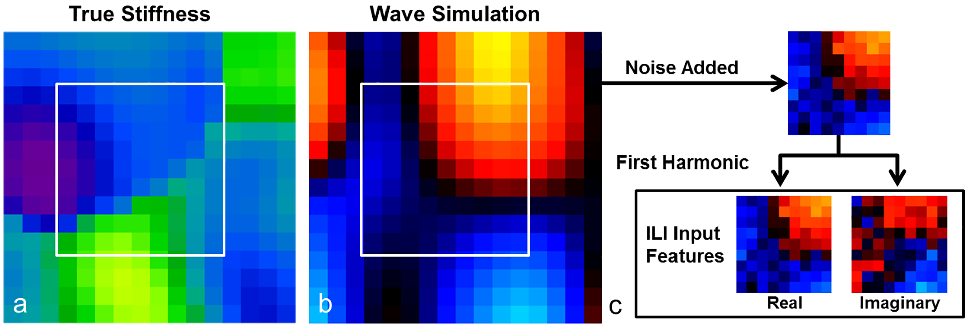
(a) Piecewise smooth input stiffness maps are generated by smoothing 3D Gaussian noise fields with 3D Gaussian kernels of randomly chosen x, y, and z dimensions. (b) Point-source wave sources are placed at the boundary of the simulation and the forward problem is solved to generate a wave image. (c) A 9×9×9 voxel patch, one such patch shown in the white square in (a) and (b), is taken from near the center of the simulation. The temporal first harmonic is taken after each patch has had noise added to generate the input features for the neural network.

After each dataset had been generated, a cubic patch was selected from the center of the simulation. For data sets with inclusions, the sharp transition was included in the patch. Zero-mean Gaussian noise was added to each patch of training data with a standard deviation scaled to assign the patch a median signal to noise ratio in the range 1 to 20 (uniform distribution). The input features to the artificial neural network were the real and imaginary components of the temporal first harmonic of the voxels in each patch. The real and imaginary components receive the same scaling, such that no value in either the real or imaginary component had an absolute value greater than 1.

2.2. Inhomogeneous Learned Inversion (ILI)

The 3D convolutional neural network architecture used includes inception blocks and residual connections and has been described previously (Murphy et al., 2020). The network was fit using the Adam optimizer (Kingma and Ba, 2017) with a mean squared error (MSE) loss function. Weights were updated after processing batches of 1000 training examples. Three decreasing learning rates were used, and training at each learning rate was stopped after three consecutive iterations where the MSE did not improve in the validation set. The output of the network was a single stiffness estimate, with stiffness defined as the product of density and the square of the wave speed, assigned to the voxel at the center of the patch.

2.3. Footprint Selection

In MRE inversion with homogenous algorithms, smaller patches are desirable (for higher resolution), but larger patches may be required to sufficiently reduce noise. In the proposed framework, we expect patch size to have little effect on resolution and for large patches to offer improved performance in noisy data. However, large patches will increase the likelihood of edge artifacts when the processing footprint overlaps with voxels outside the tissue of interest (such as cerebrospinal fluid and skull in brain MRE). For this reason, as well as the computational cost associated with increasing patch size, we limited our maximum side length to 9 voxels. To ensure we chose the optimal footprint within that limitation, 5 million 3-dimensional simulated datasets were generated, and separate ANNs were trained as described above using cubic training patches with side lengths of 5, 7, and 9 voxels. An additional 250,000 simulated datasets were generated to serve as the validation set, and 30,000 simulated datasets were generated for the test set. Each network was evaluated on its test set by determining the correlation coefficient between the inversion estimate and the true stiffness at the center of the patch after the addition of noise. The ANN with a 9×9×9 voxel cubic footprint performed best in the test set and is used for all future analyses.

2.4. Performance in the Test Set

Model evaluation was performed on the 30,000 examples in the test set. The correlation coefficient was computed between the stiffness estimate and the true stiffness at the center of the patch for each example in the test set using three inversion algorithms:

1. Direct Inversion with quartic smoothing of the displacement images prior to inversion (Romano et al., 2000).

2. Homogeneous learned inversion (HLI): our term for a neural network inversion trained on patches of homogeneous data simulated using point-source sinusoids with attenuation as described in (Murphy et al., 2020).

3. ILI: the neural network inversion described above.

As DI is prone to outliers that would impact the correlation coefficient, examples where the DI stiffness estimate exceeded 30 kPa were removed for the DI results only. This analysis was performed both before and after the addition of noise. DI with 3×3×3, 5×5×5, 7×7×7, and 9×9×9 quartic smoothing kernels was evaluated, as well as HLI footprints of 5×5×5, 7×7×7, and 9×9×9. As with ILI, the footprint for each algorithm that provided the best performance in the test set is used for all further analyses. Quartic smoothing with a 9×9×9 kernel for DI (11-voxel total footprint), and a footprint of 9×9×9 for HLI provided the best results in the test set and are used in all figures for all experiments unless otherwise stated. The larger DI footprint was tested because the convolution of a 7×7×7 filter with the Laplacian kernel used in DI does not result in a full 9×9×9 cube, and was selected because the DI result in noisy data continued to improve with a 9×9×9 filter (Table 1).

Table 1. Inversion performance in the ILI test set.

Pearson correlation coefficient between the inversion estimate and true stiffness at the center of the patch. Noisy data had SNRs ranging from 1 to 20.

	DI		HLI		ILI
Spatial Footprint	Noise-free	Noisy	Noise-free	Noisy	Noise-free	Noisy
5×5×5	0.749	0.387	0.801	0.657	0.904	0.785
7×7×7	0.768	0.605	0.811	0.756	0.967	0.904
9×9×9	0.758	0.685	0.821	0.798	0.979	0.94
11×11×11	0.728	0.707

2.5. Coupled Harmonic Oscillator Simulation Experiments

Inversion algorithms were then evaluated in a set of simulation experiments to investigate the effects of noise and stiffness inhomogeneity on the accuracy of stiffness estimation. The CHO simulation was used to generate 2 sets of 1000 41×41×41 voxel simulated datasets with all parameters as described in section 2.1 except for the stiffness profile. The first experiment used simulations of homogeneous patches with stiffness chosen randomly from a uniform distribution of 1 to 15kPa to generate a noise-free dataset. The effect of noise was investigated by adding zero-mean Gaussian noise to adjust the median SNR in each simulation to values of 5 and 20. As there is attenuation within these simulations the SNR varies across an image. The second experiment added inclusions with diameters ranging from 1 to 5 cm with background and inclusion stiffness randomly selected from a uniform distribution of 0.5 to 15kPa. As in the homogeneous simulations, noise was added to generate two additional datasets where the median SNR in the inclusion was 5 or 20. We evaluated the same three inversion algorithms described above on these simulations.

For the homogeneous experiments, the root mean squared error (RMSE) between the median of a centered 35×35×35 patch from each inversion and the known true stiffness value is reported. To investigate voxel-level stability, the interquartile range (IQR) of the voxel-level percent error is reported from the same centered patch. This smaller patch size was used to ensure that the harmonic force generators and voxels directly adjacent would not be located within the patch. For the inclusion experiments, the RMSE between the median of the inclusion from each inversion and the known true stiffness values of the inclusion is reported. The inclusion mask applied to the inversion results did not include any partial volume voxels in the true stiffness map at the edge of the inclusion.

2.6. Phantom Experiment

To assess the performance of ILI on real data, MRE was performed on a polyvinyl chloride (PVC) brain phantom containing six spherical inclusions with diameters of 1.75cm, 2cm, 2.25cm, 2.5cm, 2.75cm, and 3cm. The 50% PVC/50% softener background has a stiffness of 3.42kPa (at 60Hz) and the 65% PVC/35% softener inclusions have a stiffness of 7.09kPa as measured on a RheoSpectris C500+ (Rheolution, Inc., Montreal, QC, Canada) on samples poured from the same batch as the MRE phantom. Mechanical vibration was applied via a pneumatic system with power levels of 3, 5, and 7 percent to produce wave data with varying SNR (Resoundant Inc., Rochester, MN). Scanning was performed on a compact 3T system with a high performance gradient capable of 80 mT/m amplitude and 700T/m/s slew rate (Foo et al., 2018) using a modified GRE pulse sequence with the following parameters: 7.2 mT/m motion encoding gradient (MEG) amplitude, mechanical vibration=60Hz, TE=20.4ms, TR=24.1ms, one 16.7 ms first-moment nulled MEG cycle, motion encoding sensitivity (MENC) = 7.1 μm/rad, BW=±25kHz, FOV=240×240×192mm³, acquisition matrix= 120×120×96, flip angle = 12°, 2D GRAPPA acceleration=2, 8 channel receiver array (Invivo, Gainesville, FL), scan time=12:25.

ILI, HLI, and DI were applied to the first harmonic of the curl of the measured displacement field. ILI and HLI results were analyzed and displayed without any further filtering or smoothing. DI results were median filtered with a 3×3×3 kernel for display only. Contrast to noise ratio (CNR) as defined in (Doyley et al., 2003) is reported for all three inversions. Note that for DI, CNR was calculated using the median values of the inclusion and background to minimize potential bias due to outliers. To statistically test for differences in CNR, two linear mixed effects models were fit with CNR as the response variable. The full model included fixed effects of inversion, driver power, inclusion diameter and a constant, with random slopes (inversion and inclusion diameter) and intercepts for each driver power. The restricted model was identical with the exception that the fixed effect of inversion was removed. The likelihood ratio test was then used to test if inclusion of inversion as a fixed effect significantly improved the prediction of CNR (p<0.05 considered significant).

To evaluate the performance of each inversion at the boundaries of the inclusions, a line profile across the boundary was fit. A map of distance (in voxels) from the inclusion boundary was developed by repeated dilations (distance from the boundary into the background) or erosions (distance from the boundary into the inclusion) of the inclusion masks using a 6-connected jack-shaped structural element. For each distance from the boundary, the median stiffness as well as the 97.5 and 2.5 percentiles were estimated by a 1000 sample bootstrap with case resampling (treating inclusions as cases). Similar to the CNR test, two linear mixed effects models were fit with the error in squared stiffness estimates as the response variable. To reduce the number of model parameters, a restricted cubic spline basis was used to represent position with respect to the boundary (3 knots located 3 voxels into the background, on the boundary, and 3 voxels into the inclusion). The full model included inversion, position, and their interaction as fixed effects, with random slopes (inversion, position, and their interaction) and intercepts for each inclusion. The restricted model was identical with the exception that the fixed effects involving inversion were removed. The likelihood ratio test was again used to test if inclusion of inversion as a fixed effect significantly improved the prediction of the squared error in stiffness estimates (p<0.05 considered significant).

2.7. In Vivo Evaluation

Human data were obtained with institutional review board approval and written informed consent from all patients. Meningiomas offer an opportunity to assess the accuracy of ILI in vivo as they are well defined lesions with clear borders and their stiffness is known qualitatively from the surgical report at resection. Since meningiomas have high variability in stiffness, we consider a subset of tumors stiffer than normal brain to allow cross-subject analysis of the spatial pattern of stiffness changes. Of the 64 meningioma cases with available surgical reports in our MRE database, 23 were stiff enough that suction could not be used for removal of any part of the tumor (encompassing scales 3, 4, and 5 described in (Hughes et al., 2015)). Of these 23, one case was excluded because of a T1-weighted (T1w) image of insufficient quality to accurately segment the meningioma and two cases were excluded because of extensive tumor growth into the sinuses. After generating the stiffness maps but before any further processing, three additional cases were excluded because the median tumor stiffness for DI was softer than normal brain. All three of these cases were highly vascular tumors, where the surgical score, which is dependent on the surgical instrumentation used to resect the tumor, is more likely to be discordant with MRE measured stiffness (Hughes et al., 2015). Seventeen cases were included in the final analysis.

MRE data were acquired as described in (Hughes et al., 2015) with 3mm isotropic resolution and 8 phase offsets sampled over one period of 60Hz motion on clinical 3T scanners (GE Medical Systems, Milwaukee, WI) or the compact 3T scanner described above (Foo et al., 2018). MRE data were resampled to 2mm isotropic resolution prior to computation of the curl and subsequent inversion to allow the use of the same ILI and HLI networks used in sections 2.4–2.6. Tumor segmentation was performed manually on a T1w image acquired in the same session as the MRE scan (acquisition previously described in (Murphy et al., 2013b)) using FSLView (Jenkinson et al., 2012). Gray matter, white matter, and cerebrospinal fluid probability maps were computed in SPM5 (Ashburner and Friston, 2005). Then the T1w image, along with the tissue probability maps and tumor mask, were registered to the MRE magnitude image, and the T1w image and all derived masks were resampled to 2mm isotropic resolution. ILI, HLI, and DI were applied to the first harmonic of the curl of the resampled MRE displacement images.

To assess overall spatial agreement between manual tracings and a stiffness-based segmentation, stiffness maps for each inversion in each subject were thresholded at the 95^th percentile of the normal brain stiffness, and the Dice coefficient was calculated between the thresholded stiffness map within the tumor mask and the tumor mask itself. To compute the stiffness threshold, the gray and white matter probability maps were summed and all voxels with a combined probability greater than or equal to 95% that were outside the tumor mask were defined as normal brain. To reduce bias introduced by edge effects, two erosions using a 6-connected jack-shaped structural element were performed on the resulting segmentation. The 95^th percentile within this volume was then used to threshold the stiffness map. Paired, two-tailed T-tests were used to compare Dice coefficients between ILI and DI and ILI and HLI (p<0.05 considered significant).

To assess inversion performance at the tumor boundaries, similar analysis to that in section 2.6 was used. A map of distance (in voxels) from the tumor boundary was developed by repeated dilations (distance from the boundary into the brain) or erosions (distance from the boundary into the tumor) of the tumor mask using a 6-connected jack-shaped structural element. For each subject, the median stiffness at each location for each inversion was used to generate a summary line profile across the tumor boundary. The maximum and minimum values of this line profile were used to scale each line profile from 0 to 1 so that data from all subjects (with varying stiffness both in tumor and surrounding brain) could be combined to evaluate the shape of the median stiffness estimate across the tumor boundary. Using the combined data, for each distance from the boundary the median stiffness as well as the 2.5 and 97.5 percentiles were estimated by a 1000 sample bootstrap with case resampling (treating subjects as cases).

All stiffness maps have been interpolated 2-fold for display purposes only.

3. Results:

3.1. Performance in Test set

Results in the test set using the best performing spatial footprint in the noisy test set for each inversion are summarized in Figure 2. In the noise-free case, all three inversion estimates correlate with the true stiffness, with ILI showing the strongest correlation (R=0.979, R=0.821, and R=0.728 for ILI, HLI, and DI, respectively). This result shows that ILI improves estimation accuracy of spatially varying stiffness. ILI (R=0.940) continues to provide higher correlation than HLI (R=0.798) and DI (R=0.707) with noise added. Results using all tested spatial footprints are shown in Table 1.

Figure 2. ILI is more accurate than HLI and DI in its test set.

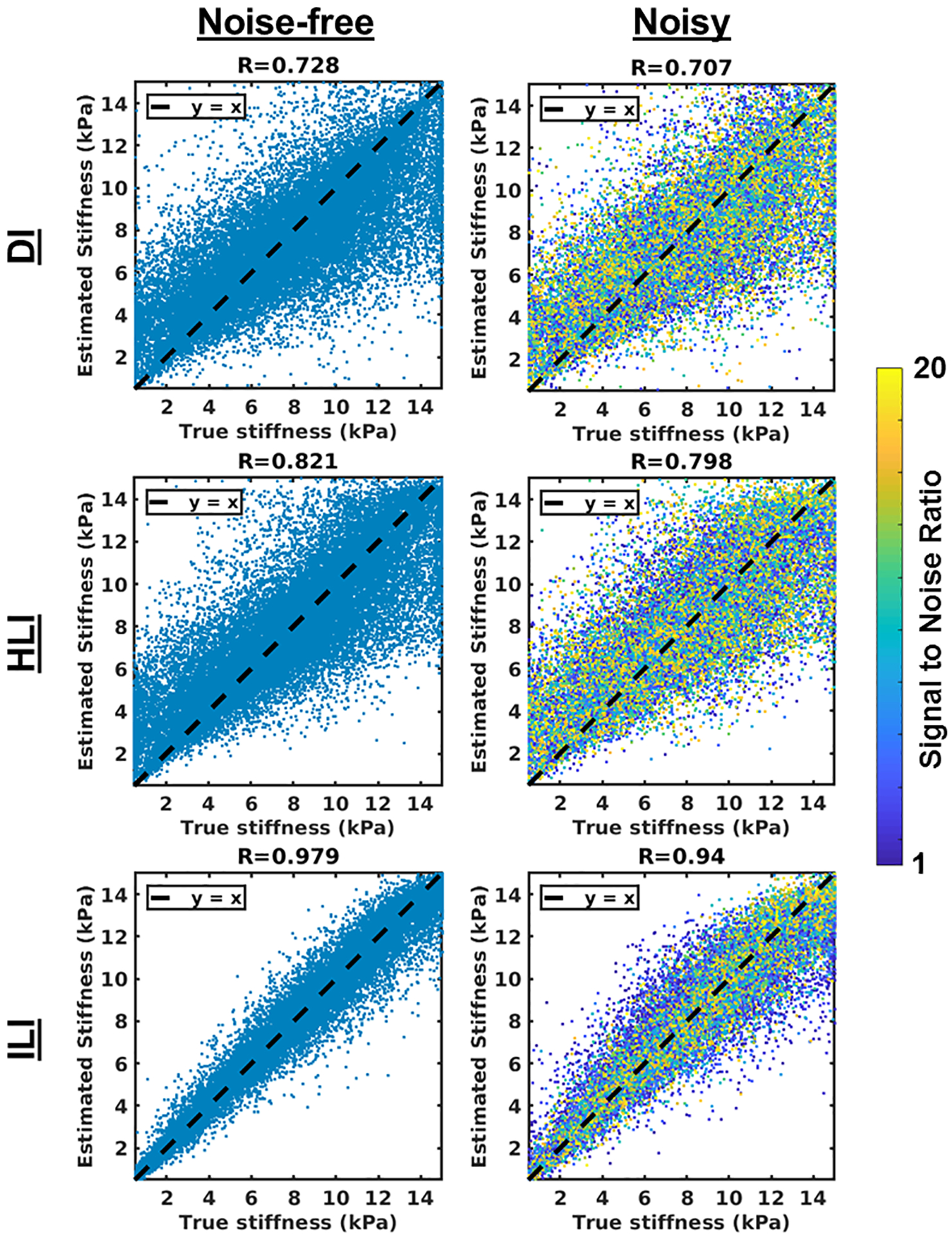
DI, top row, HLI, middle row, and ILI, bottom row, results in a test set of 30,000 patches. Results for noise-free patches (first column) and noise added patches (second column) are shown. The spatial footprint that maximized the correlation coefficient in the noisy case is shown for each inversion (11×11×11 for DI, 9×9×9 for HLI, and 9×9×9 for ILI).

3.2. CHO simulations

Results from the CHO experiments using all tested spatial footprints for all three inversions are summarized in Table 2. Briefly, ILI with a 9×9×9 spatial footprint provided more accurate estimates of inclusion stiffness in noisy data than DI or HLI of any tested spatial footprint. With the smallest spatial footprint tested (5×5×5 voxels), HLI provided the most accurate stiffness estimates in the high noise homogeneous dataset. In low noise and noise-free datasets, DI provided the most accurate stiffness estimates in homogeneous data. For 5×5×5 and 7×7×7 voxel footprints, the learned inversions provide lower variance stiffness estimates in noisy homogeneous simulations than DI. Figure 3 allows visualization of the partial volume effect induced by the homogeneity assumption in HLI and DI with large footprints. As inclusion size decreases, HLI and DI stiffness estimates move closer to the no contrast line. This effect is mitigated by ILI.

Table 2. Inversion estimate accuracy in CHO simulations.

Root Mean Square Error (RMSE, kPa) between median stiffness and true stiffness of the entire patch (homogeneous simulations) and the inclusion (inclusion simulations). The mean across all simulations of the interquartile range (IQR) of the voxel-level percent error in each simulation is reported as IQR. Inclusion diameter ranged from 1 to 5 cm. SNRs are median values in the 41×41×41 patch.

RMSE In Inclusion Experiment
	DI			HLI			ILI
Spatial Footprint	Noisefree	SNR20	SNR5	Noisefree	SNR20	SNR5	Noisefree	SNR20	SNR5
5×5×5	7.19E-10	3.7328	5.4256	1.3362	1.7725	3.0137	1.2373	1.5792	2.7431
7×7×7	0.9834	1.7884	4.0786	1.8134	1.854	2.3575	1.2368	1.3431	1.7192
9×9×9	1.9016	2.0078	2.9958	2.2744	2.2963	2.4481	1.0537	1.139	1.6173
11×11×11	2.5865	2.6144	2.8483
RMSE in Homogeneous Experiment
	DI			HLI			ILI
Spatial Footprint	Noisefree	SNR20	SNR5	Noisefree	SNR20	SNR5	Noisefree	SNR20	SNR5
5×5×5	3.99E-10	0.5044	3.1563	0.5345	0.7375	1.5011	0.7623	0.9234	1.8283
7×7×7	3.99E-10	0.05	0.614	0.2737	0.3518	0.8082	0.4059	0.492	0.8934
9×9×9	3.99E-10	0.0099	0.1234	0.2257	0.2562	0.4568	0.3748	0.4231	0.6769
11×11×11	4.10E-10	0.048	0.2092
IQR in Homogeneous Experiment
	DI			HLI			ILI
Spatial Footprint	Noisefree	SNR20	SNR5	Noisefree	SNR20	SNR5	Noisefree	SNR20	SNR5
5×5×5	2.80E-12	0.3245	0.7177	0.0914	0.1687	0.4061	0.1087	0.1955	0.4921
7×7×7	2.80E-12	0.0963	0.345	0.0646	0.1043	0.2659	0.0833	0.1309	0.3094
9×9×9	2.81E-12	0.0381	0.1497	0.0535	0.079	0.1902	0.0861	0.1328	0.2902
11×11×11	3.57E-12	0.0331	0.1219

Figure 3. Summary results from Coupled Harmonic Oscillators (CHO) experiment.

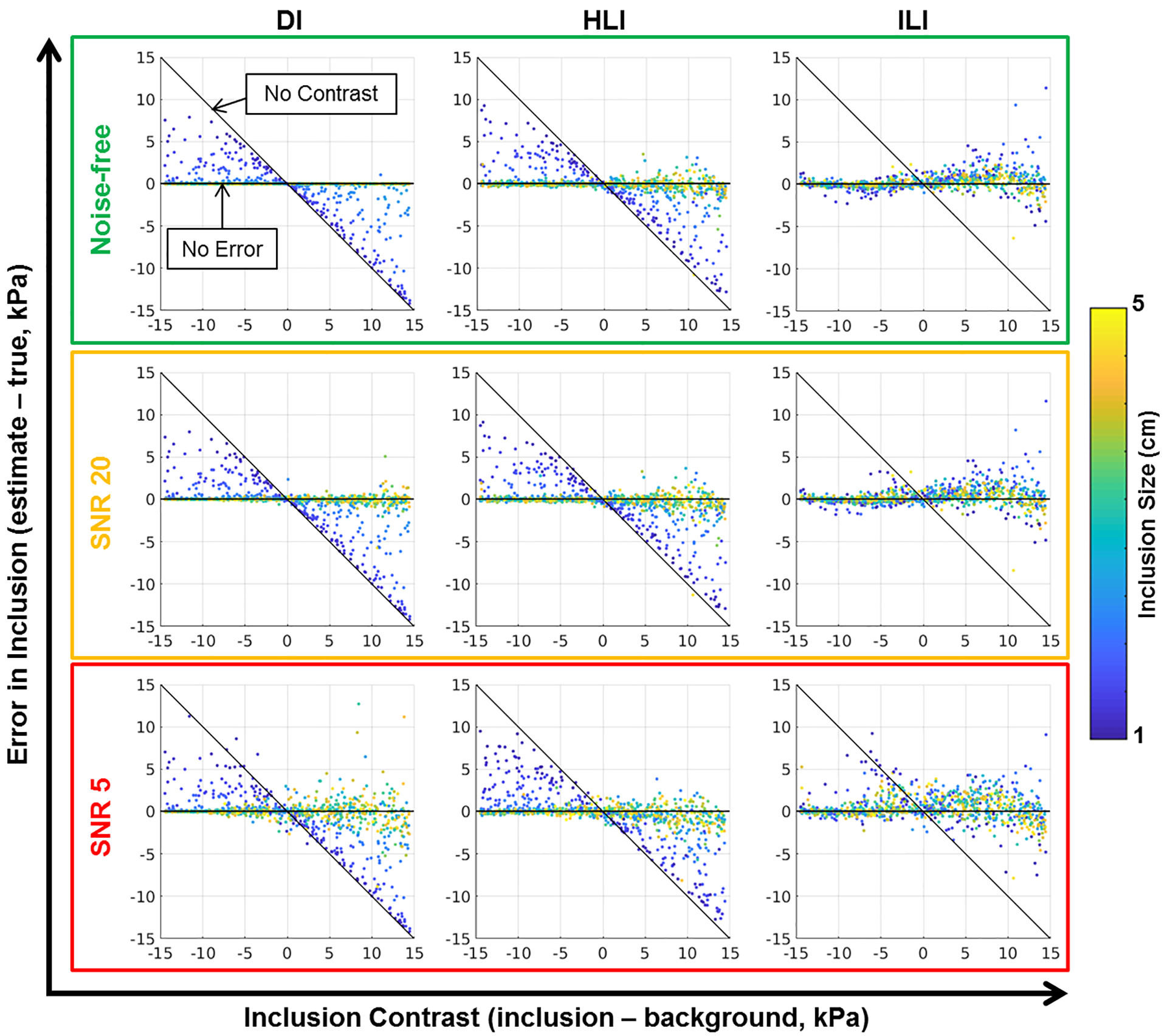
Each plot shows the error in inclusion estimate (estimated stiffness in the inclusion - true stiffness in inclusion) vs the inclusion contrast (true inclusion stiffness - true background stiffness) in 1000 CHO simulations. For a perfect inversion all points would be along the zero-error line. If an inversion completely fails to detect the inclusion points will be along the diagonal labeled “No Contrast”. The color of the data points corresponds to inclusion size.

3.3. Phantom Experiment

Phantom inversions of the 7 percent driver power scan are shown in Figure 4. ILI (9×9×9 spatial footprint) more clearly delineates the 1.75cm, 2cm, and 2.25cm diameter inclusions than HLI (9×9×9 spatial footprint), and inclusions <2.5 cm in diameter are difficult to detect with DI (11×11×11 spatial footprint). ILI also shows a higher CNR than HLI and DI for all inclusions at all driver power levels (Figure 5). The likelihood ratio test showed that the linear mixed effects model including inversion as a fixed effect significantly improved prediction of CNR (p=0.001). Because the phantom data has high SNR, the large spatial footprints that provided optimal performance in the noisy test set are unnecessary. A footprint of 5×5×5 voxels optimized the CNR for both HLI and DI in the phantom. Inversion results with these footprints more clearly depict the inclusions than the large footprint results (Supplemental Figure1), but still provide lower CNR in all inclusions at all driver power levels than ILI with a 9×9×9 footprint (Supplemental Figure 2, p<0.01, likelihood ratio test). ILI also shows a sharper transition at the inclusion boundaries and more accurate stiffness estimates than HLI and DI with large footprints (Figure 6) or the optimal footprints for the phantom data (Supplemental Figure 3). Including inversion as a fixed effect significantly improved the prediction of errors in stiffness estimates in both cases (p<0.001 for both).

Figure 4. ILI more clearly depicts stiff inclusions in a brain-simulating phantom.

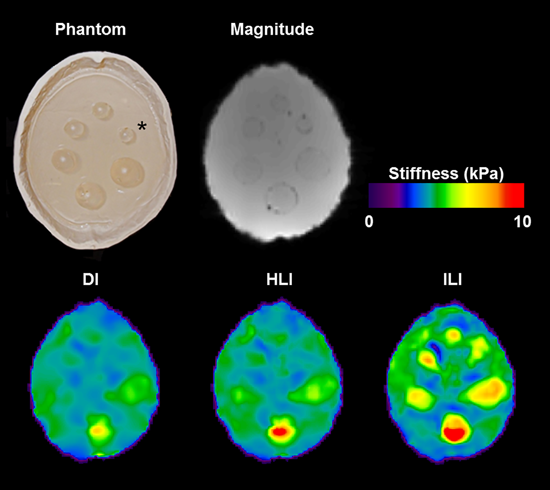
Top left: Photograph of the PVC phantom. Inclusion diameters, proceeding counter clockwise from the inclusion labeled with the asterisk, are 1.75, 2, 2.25, 2.5, 2.75, and 3cm. Top Middle: MRE magnitude image. Bottom left: Direct inversion after 3×3×3 median filtering. Bottom middle: HLI. Bottom right: ILI. The measured stiffness of the background and inclusions was 3.42 and 7.09 kPa, respectively.

Figure 5. ILI provides higher contrast to noise ratio (CNR) in the phantom.

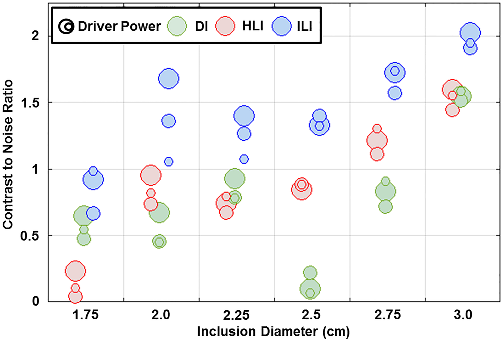
Calculated CNRs for the inversions shown in Figure 4. The size of the circles represents the driver power (3, 5 or 7 percent).

Figure 6. ILI provides sharper transitions at inclusion boundaries.

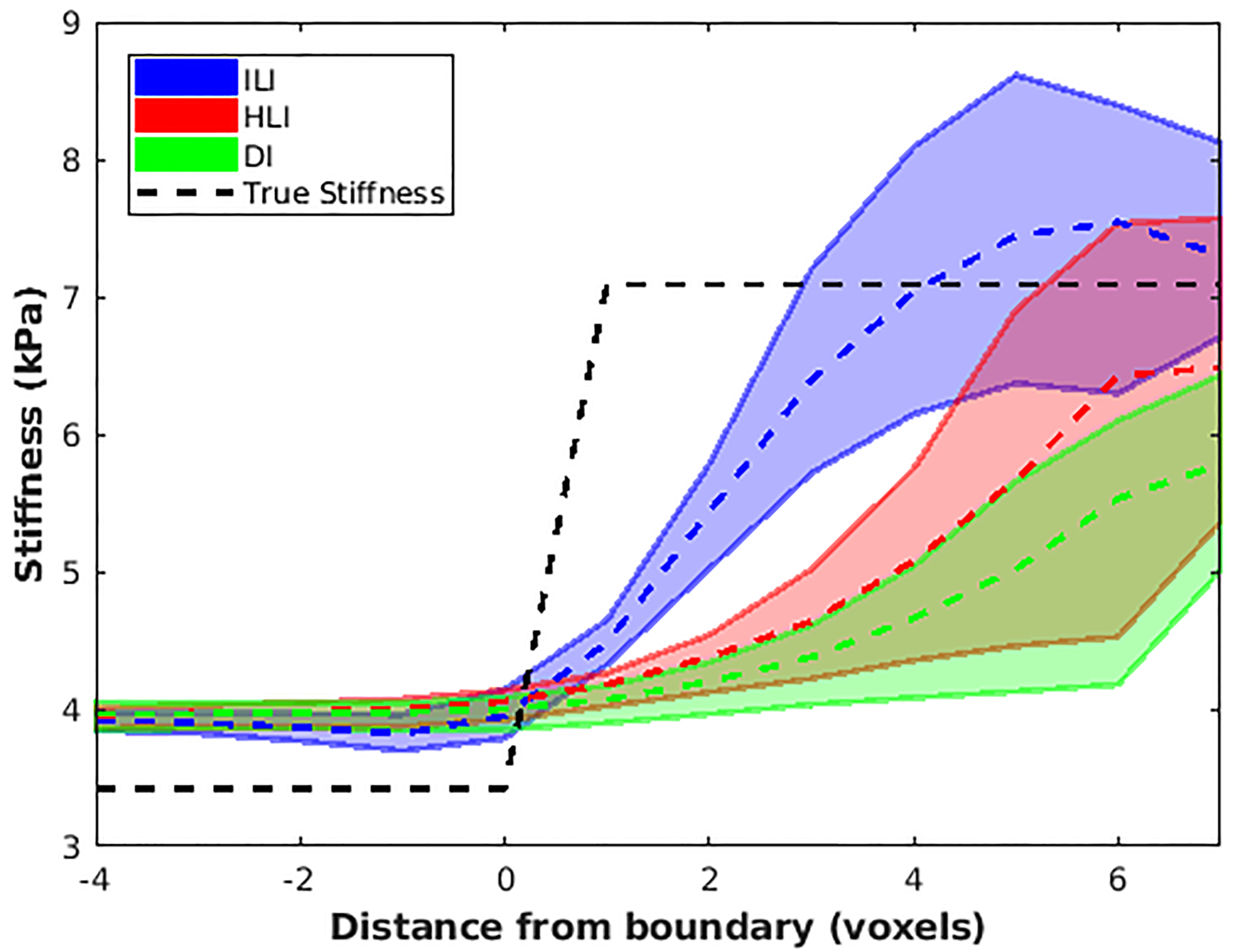
Negative values on the x-axis represent distance from the boundary into the background while positive values show distance into the inclusion. Dashed lines connect median values at each position while solid lines show the 2.5^th and 97.5^th percentiles for each inversion.

3.4. In Vivo Results

Two representative cases are shown in Figure 7. The Dice coefficient for ILI was significantly higher than for DI (p<0.001) with no significant difference between ILI and HLI (p=0.15) (Figure 8). ILI also offered sharper transition from background brain into the tumors than HLI and DI (Figure 9).

Figure 7. T1-weighted image and inversion results in two meningioma cases.

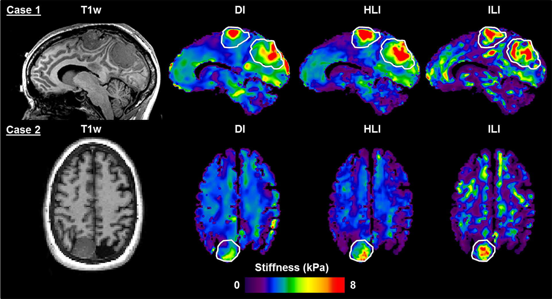
For Case 1, the superior tumor was described as stiff throughout and the posterior tumor was described as having heterogeneous stiffness on resection (only the superior tumor was included in group analysis). In Case 2, the tumor was described as very stiff throughout at resection. Regions of interest outline the tumor extent as manually traced on the T1-weighted image.

Figure 8. Dice coefficient results in 17 meningioma cases.

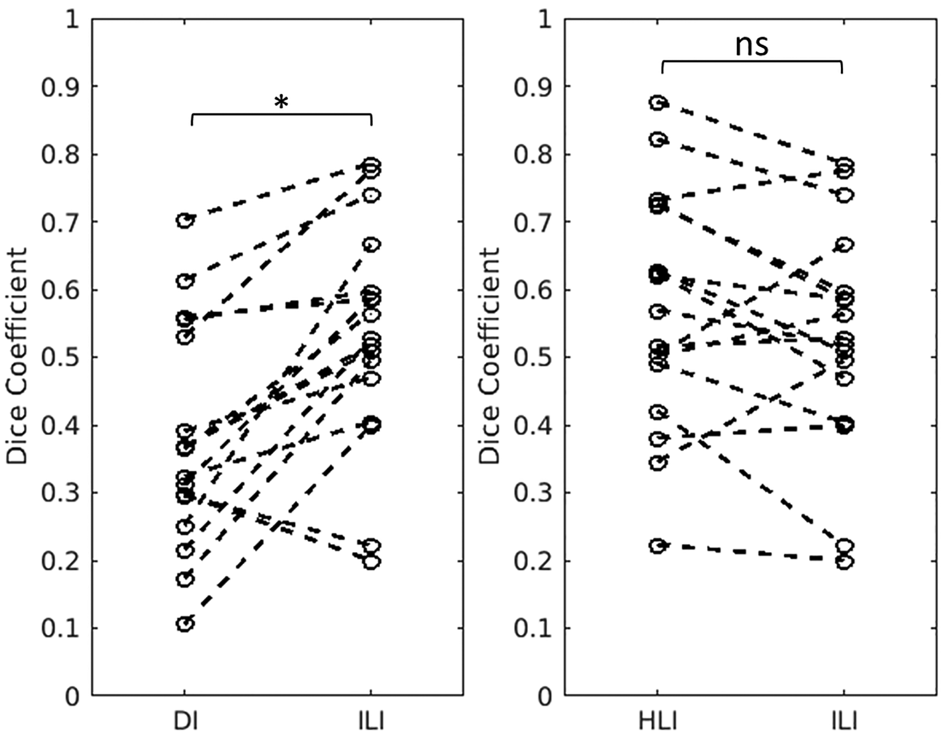
ILI produces a significantly higher Dice coefficient than DI with 9×9×9 quartic smoothing. There is no significant difference between HLI and ILI Dice coefficients (p=0.15). Dashed lines connect the individual cases across the inversions. *p<0.001, ns = nonsignificant, two-tailed paired t-tests.

Figure 9. ILI provides sharper transitions at boundaries of stiff tumors in vivo.

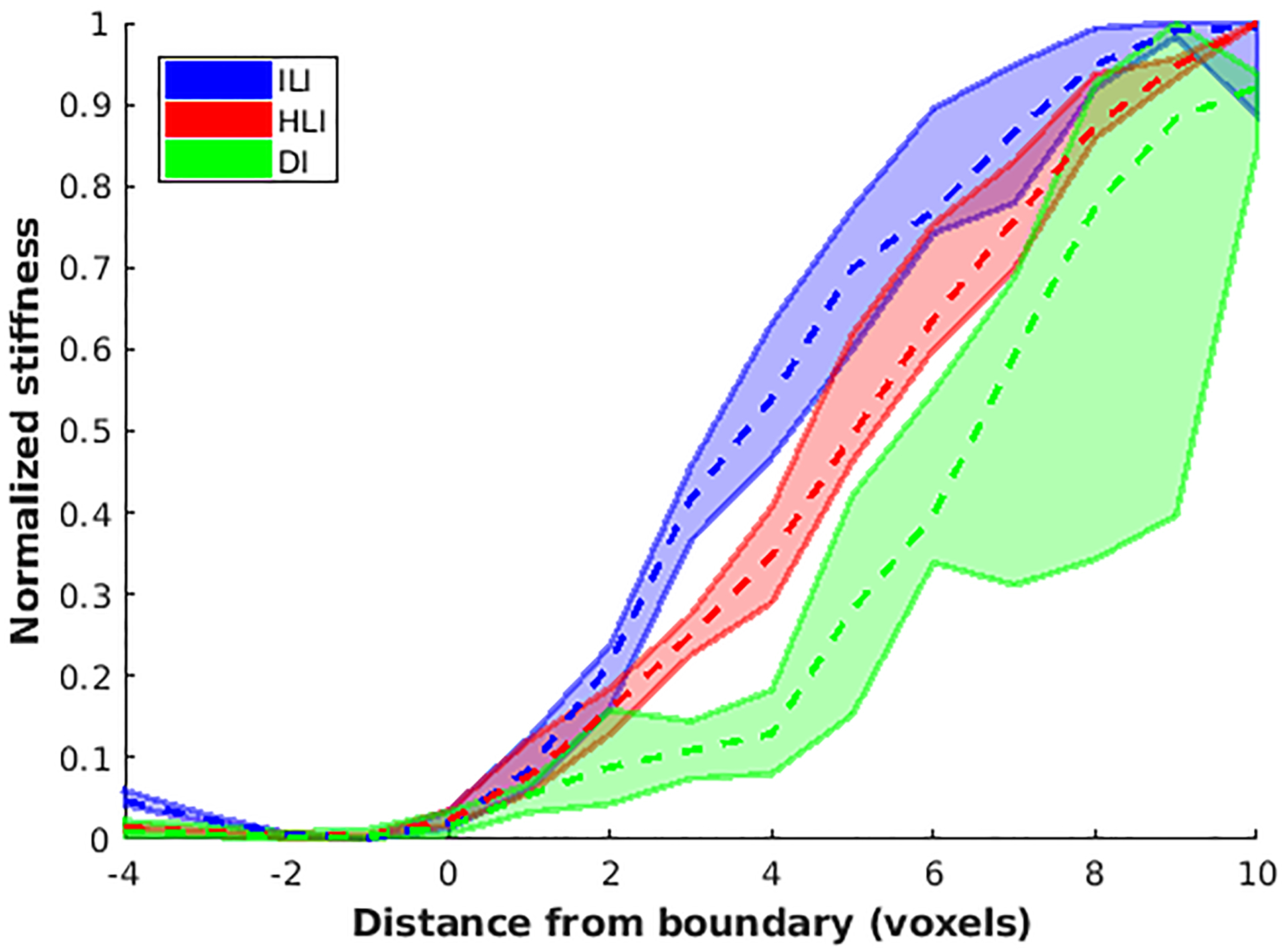
Negative values on the x-axis represent distance from the boundary into normal brain while positive values show distance into the tumor. The zero position is the first voxel labeled as tumor. Dashed lines connect median values at each position while solid lines show the 2.5th and 97.5th percentiles for each inversion.

4. Discussion:

This study builds upon recently reported work showing the feasibility of using artificial neural networks for inversion in MRE (Murphy et al., 2018) by increasing the complexity of the training data using a coupled harmonic oscillator simulation (Sack et al., 2002) of shear wave propagation in a medium with inhomogeneous stiffness, thereby more closely simulating true tissue mechanical properties. This advance in the training data improves the accuracy of stiffness estimation in the presence of material inhomogeneity.

Experiments in small patches of simulated wave data showed that ILI was more accurate than DI and HLI at estimating the stiffness of voxels in areas of spatially varying stiffness (Figure 2). This result is expected as DI is known to break down at boundaries (McGrath et al., 2016; Murphy et al., 2013b). ILI accuracy decreased with decreasing SNR, but there does not appear to be any consistent bias in estimates of noisy data except at the top of the training range, where ILI estimates are biased soft in the noisiest examples (Figure 2). Both HLI and DI show no clear trend with SNR (right column, Figure 2), and produce estimates biased toward the center of the training range, suggesting that at the spatial footprints shown these methods are more affected by their assumption of material homogeneity than SNR.

Additional, larger-footprint simulation experiments showed that the median stiffness of an inclusion estimated by ILI was more accurate than estimates by DI and HLI at multiple noise levels. The perfect performance (to numerical precision) of DI in the homogeneous, noise-free simulation (Table 2) serves as an important check that the simulation produces accurate displacement fields that obey the fundamental assumptions of conventional inversion algorithms under ideal conditions. In noise-free simulations with inclusions, DI accurately estimated the stiffness of large inclusions, with errors only in the smaller inclusions (Figure 3). This is expected, as with decreasing inclusion size, the proportion of voxels affected by the boundary will increase. Due to the partial volume effect, this will result in underestimated stiffness of a stiff inclusion in a soft background and overestimated stiffness of a soft inclusion in a stiff background. This effect can be seen in both the DI and HLI panels of Figure 3. These partial volume effects are substantially reduced by ILI, though ILI actually appears to overestimate inclusion contrast in some of the smallest inclusions when SNR is high. With the large spatial footprints used in Figure 3, all three inversion algorithms appear robust to noise, with relatively little change in performance as noise is added. However, when using smaller spatial footprints (Table 2), it is clear that DI is more sensitive to noise than the ANN inversions, which is in agreement with previous findings (Murphy et al., 2018).

Results in the phantom suggest that ILI improves the detectability of focal inclusions, producing higher CNR than DI and HLI in six inclusions of 1.75 to 3cm in diameter (Figure 5 and Supplemental Figure 1). Further, ILI provided sharper boundaries at the edges of inclusions (Figure 6 and Supplemental Figure 3). As would be expected due to the assumption of local homogeneity, DI and HLI blur inclusion boundaries more with larger spatial footprints (Figure 5 versus Supplemental Figure 1).

In the meningioma cases shown (Figure 7), ILI more sharply demarcated tumor boundaries. ILI also shows focal areas of increased stiffness in presumably normal brain when compared to the HLI and DI stiffness maps. While this study is not designed to assess the accuracy of these regions, we note that the general areas where ILI shows a stiffness increase also show stiffness increases with the other two inversions, just less clearly defined and with lower stiffness estimates. Further studies are needed to assess the performance of ILI in normal brain. The large stiffness training range used in this study was chosen expressly for analysis of focal inclusions and tumors, and more accurate estimates in normal brain would likely be achieved using a smaller training range.

In the cross-subject in vivo experiment, ILI produced a higher Dice coefficient, labeling more of each tumor as stiff, than DI, but not HLI (Figure 8). This equivalency of HLI and DI may be due to the methodology used to set a threshold for what qualifies as stiffer than normal brain. We chose to use the 95^th percentile of normal brain values, and as can be seen in Figure 7, HLI produces softer and more homogeneous estimates in normal brain than DI and ILI. As such the threshold was lower for HLI than the other two algorithms. Additionally, to perform these analyses we assume that the tumor is homogeneously stiffer than normal brain. While this may have been the surgeon’s qualitative impression at resection, it is likely that there is some heterogeneity in stiffness within the tumor. This threshold effect likely contributes to the relatively low Dice coefficients seen with all three inversions, and would have the biggest impact on ILI. HLI and DI would be expected to blur out regions of heterogeneity within the tumor, while ILI may detect them. As expected, ILI provided sharper transitions in stiffness between the normal brain and tumor than DI and HLI (Figure 9).

This study suggests that ILI potentially possesses advantages over previously described inversion algorithms. LFE techniques estimate instantaneous spatial frequency by applying a set of filters to the displacement data and developing an estimate based on the energy in each filter band (Clayton et al., 2013; Knutsson et al., 1994). It also assumes local homogeneity and has limited spatial resolution (Manduca et al., 2001). Most DI techniques, which solve the equations of motion in a viscoelastic medium (Oliphant et al., 2001; Papazoglou et al., 2008; Romano et al., 1998), assume homogeneity (Manduca et al., 2001). As they rely on second derivatives, their major drawback is voxel-level numerical instability, especially in the presence of noise, which requires additional filtering of the displacement data that negatively impacts spatial resolution. One recent approach has removed the local homogeneity assumption, but at the cost of requiring MRE data at multiple frequencies, which would increase scan time (Barnhill et al., 2018). Another approach uses a finite element based inversion technique that does not assume homogeneity but needs further evaluation in vivo (Honarvar et al., 2013). Nonlinear inversion is an iterative technique that uses finite element models to jointly estimate displacements and tissue mechanical parameters within subzones of the displacement image (McGarry et al., 2012; Van Houten et al., 2001). It does not assume local homogeneity. An adaptation to NLI adds soft prior regularization, which incorporates spatial information into the inversion by penalizing heterogeneity within specified subregions (McGarry et al., 2013). The spatial information comes from a segmentation that is provided to the algorithm. This method can produce sharp stiffness gradients at boundaries and decrease measurement uncertainty in small ROIs (Johnson et al., 2016; McGarry et al., 2013), but is sensitive to the underlying segmentation and favors homogeneity within some region of interest. Due to its iterative approach that requires solving many small finite element simulations, NLI reconstruction time is on the order of hours. The ILI network presented in this study took approximately 3 days to train (1 day to generate training data, and two days to train the ANN), but could reconstruct the included phantom and brain MRE studies in under 10 minutes. GPU acceleration would markedly reduce the time to invert images, and may accelerate generation of training data.

Neural network inversions (NNIs, including both HLI and ILI) could easily be implemented into a clinical workflow. Each NNI is limited to processing data at the resolution, frequency, and stiffness range at which it was trained. While it takes days to generate an NNI, it can then be used to invert any MRE data at its trained resolution and frequency when its stiffness range is appropriate. Training an NNI for a particular resolution, frequency, and stiffness range is simply accomplished by adapting the parameters in the CHO simulations used to generate training data. Further, as was done in this study for the in-vivo data, MRE data acquired at a different resolution could be resampled to the resolution of the NNI before inversion. In practice, acquisition parameters of MRE protocols for specific applications remain mostly constant over time, and after an initial set of NNIs has been trained for regularly acquired frequencies and resolutions, the need to train new NNIs should be infrequent.

The primary limitation of this study is in the CHO simulation used to generate training data. The CHO simulation has important limitations, and it is possible that training an ANN on simulated wave data from a model obeying the full Navier equations of motion in linear elastic materials would offer improved results. Particularly pertinent to this study, the CHO simulation does not contain longitudinal waves, and as such cannot accurately simulate mode conversion at interfaces. We selected the CHO model because it can be solved more rapidly, providing a sufficiently sized training set in a reasonable period of time. Despite its simplicity, our results indicate that the CHO model is accurate enough to offer an improvement over existing inversion algorithms, and the incorporation of a model obeying the Navier equations for linear elastic materials that provides the full vector displacement field is a planned future direction.

We also note that ANNs are inherently good at interpolation and bad at extrapolation. This is potentially beneficial in MRE, as it produces a stable inversion, but it does limit accurate parameter estimation to the range used to train the ANN. This makes NNI-based stiffness estimates sensitive to parameter selection. The distribution of parameters in the training set must be sufficiently wide to capture the clinical information of interest, though a parameter range that is too wide will sacrifice accuracy within the range of interest. In this study, we chose to have a maximum stiffness cutoff of 15 kPa, as the clinical utility of an estimate higher than 15 kPa is unclear in the applications presented here.

In conclusion, the results of this study confirm that neural network-based inversion algorithms for MRE can improve stiffness estimates in materials with spatially varying stiffness. These results provide motivation for further development of neural network-based inversion algorithms.

References

- Asbach P, Klatt D, Hamhaber U, Braun J, Somasundaram R, Hamm B, Sack I, 2008. Assessment of liver viscoelasticity using multifrequency MR elastography. Magn Reson Med 60, 373–379. 10.1002/mrm.21636 [DOI] [PubMed] [Google Scholar]
- Ashburner J, Friston KJ, 2005. Unified segmentation. Neuroimage 26, 839–851. 10.1016/j.neuroimage.2005.02.018 [DOI] [PubMed] [Google Scholar]
- Barnhill E, Davies PJ, Ariyurek C, Fehlner A, Braun J, Sack I, 2018. Heterogeneous Multifrequency Direct Inversion (HMDI) for magnetic resonance elastography with application to a clinical brain exam. Medical Image Analysis 46, 180–188. 10.1016/j.media.2018.03.003 [DOI] [PubMed] [Google Scholar]
- Braun J, Buntkowsky G, Bernarding J, Tolxdorff T, Sack I, 2001. Simulation and analysis of magnetic resonance elastography wave images using coupled harmonic oscillators and Gaussian local frequency estimation. Magnetic Resonance Imaging 19, 703–713. 10.1016/S0730-725X(01)00387-3 [DOI] [PubMed] [Google Scholar]
- Chollet Francois, 2015. Keras. https://keras.io. [Google Scholar]
- Clayton EH, Okamoto RJ, Bayly PV, 2013. Mechanical properties of viscoelastic media by local frequency estimation of divergence-free wave fields. J Biomech Eng 135, 021025 10.1115/1.4023433 [DOI] [PMC free article] [PubMed] [Google Scholar]
- Doyley MM, Weaver JB, Van Houten EEW, Kennedy FE, Paulsen KD, 2003. Thresholds for detecting and characterizing focal lesions using steady-state MR elastography. Med Phys 30, 495–504. 10.1118/1.1556607 [DOI] [PubMed] [Google Scholar]
- ElSheikh M, Arani A, Perry A, Boeve BF, Meyer FB, Savica R, Ehman RL, Huston J, 2017. MR Elastography Demonstrates Unique Regional Brain Stiffness Patterns in Dementias. AJR Am J Roentgenol 209, 403–408. 10.2214/AJR.16.17455 [DOI] [PMC free article] [PubMed] [Google Scholar]
- Foo TKF, Laskaris E, Vermilyea M, Xu M, Thompson P, Conte G, Van Epps C, Immer C, Lee S-K, Tan ET, Graziani D, Mathieu J-B, Hardy CJ, Schenck JF, Fiveland E, Stautner W, Ricci J, Piel J, Park K, Hua Y, Bai Y, Kagan A, Stanley D, Weavers PT, Gray E, Shu Y, Frick MA, Campeau NG, Trzasko J, Huston J, Bernstein MA, 2018. Lightweight, compact, and high-performance 3T MR system for imaging the brain and extremities. Magn Reson Med 80, 2232–2245. 10.1002/mrm.27175 [DOI] [PMC free article] [PubMed] [Google Scholar]
- Gerischer LM, Fehlner A, Köbe T, Prehn K, Antonenko D, Grittner U, Braun J, Sack I, Flöel A, 2018. Combining viscoelasticity, diffusivity and volume of the hippocampus for the diagnosis of Alzheimer’s disease based on magnetic resonance imaging. NeuroImage: Clinical 18, 485–493. 10.1016/j.nicl.2017.12.023 [DOI] [PMC free article] [PubMed] [Google Scholar]
- Honarvar M, Sahebjavaher R, Sinkus R, Rohling R, Salcudean SE, 2013. Curl-Based Finite Element Reconstruction of the Shear Modulus Without Assuming Local Homogeneity: Time Harmonic Case. IEEE Transactions on Medical Imaging 32, 2189–2199. 10.1109/TMI.2013.2276060 [DOI] [PubMed] [Google Scholar]
- Hughes JD, Fattahi N, Van Gompel J, Arani A, Meyer F, Lanzino G, Link MJ, Ehman R, Huston J, 2015. Higher-Resolution Magnetic Resonance Elastography in Meningiomas to Determine Intratumoral Consistency. Neurosurgery 77, 653–659. 10.1227/NEU.0000000000000892 [DOI] [PMC free article] [PubMed] [Google Scholar]
- Huwart L, Sempoux C, Salameh N, Jamart J, Annet L, Sinkus R, Peeters F, ter Beek LC, Horsmans Y, Van Beers BE, 2007. Liver Fibrosis: Noninvasive Assessment with MR Elastography versus Aspartate Aminotransferase–to-Platelet Ratio Index. Radiology 245, 458–466. 10.1148/radiol.2452061673 [DOI] [PubMed] [Google Scholar]
- Jenkinson M, Beckmann CF, Behrens TEJ, Woolrich MW, Smith SM, 2012. FSL. NeuroImage, 20 YEARS OF fMRI 62, 782–790. 10.1016/j.neuroimage.2011.09.015 [DOI] [PubMed] [Google Scholar]
- Johnson CL, McGarry MDJ, Gharibans AA, Weaver JB, Paulsen KD, Wang H, Olivero WC, Sutton BP, Georgiadis JG, 2013. Local mechanical properties of white matter structures in the human brain. Neuroimage 79, 145–152. 10.1016/j.neuroimage.2013.04.089 [DOI] [PMC free article] [PubMed] [Google Scholar]
- Johnson CL, Schwarb H, D J McGarry M, Anderson AT, Huesmann GR, Sutton BP, Cohen NJ, 2016. Viscoelasticity of subcortical gray matter structures. Hum Brain Mapp 37, 4221–4233. 10.1002/hbm.23314 [DOI] [PMC free article] [PubMed] [Google Scholar]
- Kingma DP, Ba J, 2017. Adam: A Method for Stochastic Optimization. arXiv:1412.6980 [cs]. [Google Scholar]
- Knutsson H, Westin CF, Granlund G, 1994. Local multiscale frequency and bandwidth estimation, in: Proceedings of 1st International Conference on Image Processing. Presented at the Proceedings of 1st International Conference on Image Processing, pp. 36–40 vol.1 10.1109/ICIP.1994.413270 [DOI] [Google Scholar]
- Lipp A, Skowronek C, Fehlner A, Streitberger K-J, Braun J, Sack I, 2018. Progressive supranuclear palsy and idiopathic Parkinson’s disease are associated with local reduction of in vivo brain viscoelasticity. Eur Radiol 28, 3347–3354. 10.1007/s00330-017-5269-y [DOI] [PubMed] [Google Scholar]
- Manduca A, Oliphant TE, Dresner MA, Mahowald JL, Kruse SA, Amromin E, Felmlee JP, Greenleaf JF, Ehman RL, 2001. Magnetic resonance elastography: Non-invasive mapping of tissue elasticity. Medical Image Analysis 5, 237–254. 10.1016/S1361-8415(00)00039-6 [DOI] [PubMed] [Google Scholar]
- Abadi Martín, Agarwal Ashish, Barham Paul, Brevdo Eugene, Chen Zhifeng, Citro Craig, Corrado Greg S., Davis Andy, Dean Jeffrey, Devin Matthieu, Ghemawat Sanjay, Goodfellow Ian, Harp Andrew, Irving Geoffrey, Isard Michael, Jia Y, Jozefowicz Rafal, Kaiser Lukasz, Kudlur Manjunath, Levenberg Josh, Mané Dan, Monga Rajat, Moore Sherry, Murray Derek, Olah Chris, Schuster Mike, Shlens Jonathon, Steiner Benoit, Sutskever Ilya, Talwar Kunal, Tucker Paul, Vanhoucke Vincent, Vasudevan Vijay, Viégas Fernanda, Vinyals Oriol, Warden Pete, Wattenberg Martin, Wicke Martin, Yu Yuan, Zheng Xiaoqiang, 2015. TensorFlow: Large-Scale Machine Learning on Heterogeneous Systems. [Google Scholar]
- McGarry M, Johnson CL, Sutton BP, Van Houten EE, Georgiadis JG, Weaver JB, Paulsen KD, 2013. Including spatial information in nonlinear inversion MR elastography using soft prior regularization. IEEE Trans Med Imaging 32, 1901–1909. 10.1109/TMI.2013.2268978 [DOI] [PMC free article] [PubMed] [Google Scholar]
- McGarry MDJ, Van Houten EEW, Johnson CL, Georgiadis JG, Sutton BP, Weaver JB, Paulsen KD, 2012. Multiresolution MR elastography using nonlinear inversion. Med Phys 39, 6388–6396. 10.1118/1.4754649 [DOI] [PMC free article] [PubMed] [Google Scholar]
- McGrath DM, Ravikumar N, Wilkinson ID, Frangi AF, Taylor ZA, 2016. Magnetic resonance elastography of the brain: An in silico study to determine the influence of cranial anatomy. Magn Reson Med 76, 645–662. 10.1002/mrm.25881 [DOI] [PubMed] [Google Scholar]
- Murphy MC, Cogswell PM, Trzasko JD, Manduca A, Senjem ML, Meyer FB, Ehman RL, Huston J, 2020. Identification of normal pressure hydrocephalus by disease-specific patterns of brain stiffness and damping ratio. Investigative Radiology In Press. [DOI] [PMC free article] [PubMed] [Google Scholar]
- Murphy MC, Huston J, Glaser KJ, Manduca A, Meyer FB, Lanzino G, Morris JM, Felmlee JP, Ehman RL, 2013a. Preoperative assessment of meningioma stiffness using magnetic resonance elastography. J. Neurosurg 118, 643–648. 10.3171/2012.9.JNS12519 [DOI] [PMC free article] [PubMed] [Google Scholar]
- Murphy MC, Huston J, Jack CR, Glaser KJ, Senjem ML, Chen J, Manduca A, Felmlee JP, Ehman RL, 2013b. Measuring the Characteristic Topography of Brain Stiffness with Magnetic Resonance Elastography. PLoS One 8 10.1371/journal.pone.0081668 [DOI] [PMC free article] [PubMed] [Google Scholar]
- Murphy MC, Jones DT, Jack CR, Glaser KJ, Senjem ML, Manduca A, Felmlee JP, Carter RE, Ehman RL, Huston J, 2016. Regional brain stiffness changes across the Alzheimer’s disease spectrum. Neuroimage Clin 10, 283–290. 10.1016/j.nicl.2015.12.007 [DOI] [PMC free article] [PubMed] [Google Scholar]
- Murphy MC, Manduca A, Trzasko JD, Glaser KJ, Huston J, Ehman RL, 2018. Artificial neural networks for stiffness estimation in magnetic resonance elastography. Magn Reson Med 80, 351–360. 10.1002/mrm.27019 [DOI] [PMC free article] [PubMed] [Google Scholar]
- Muthupillai R, Lomas DJ, Rossman PJ, Greenleaf JF, Manduca A, Ehman RL, 1995. Magnetic resonance elastography by direct visualization of propagating acoustic strain waves. Science 269, 1854–1857. [DOI] [PubMed] [Google Scholar]
- Oliphant TE, Manduca A, Ehman RL, Greenleaf JF, 2001. Complex-valued stiffness reconstruction for magnetic resonance elastography by algebraic inversion of the differential equation. Magn Reson Med 45, 299–310. [DOI] [PubMed] [Google Scholar]
- Papazoglou S, Hamhaber U, Braun J, Sack I, 2008. Algebraic Helmholtz inversion in planar magnetic resonance elastography. Phys Med Biol 53, 3147–3158. 10.1088/0031-9155/53/12/005 [DOI] [PubMed] [Google Scholar]
- Pepin KM, McGee KP, Arani A, Lake DS, Glaser KJ, Manduca A, Parney IF, Ehman RL, Huston J, 2018. Magnetic resonance elastography analysis of glioma stiffness and IDH1 mutation status. AJNR Am J Neuroradiol 39, 31–36. 10.3174/ajnr.A5415 [DOI] [PMC free article] [PubMed] [Google Scholar]
- Romano AJ, Bucaro JA, Ehnan RL, Shirron JJ, 2000. Evaluation of a material parameter extraction algorithm using MRI-based displacement measurements. IEEE Transactions on Ultrasonics, Ferroelectrics, and Frequency Control 47, 1575–1581. 10.1109/58.883546 [DOI] [PubMed] [Google Scholar]
- Romano AJ, Shirron JJ, Bucaro JA, 1998. On the noninvasive determination of material parameters from a knowledge of elastic displacements theory and numerical simulation. IEEE Transactions on Ultrasonics, Ferroelectrics, and Frequency Control 45, 751–759. 10.1109/58.677725 [DOI] [PubMed] [Google Scholar]
- Rustogi R, Horowitz J, Harmath C, Wang Y, Chalian H, Ganger DR, Chen ZE, Bolster BD, Shah S, Miller FH, 2012. Accuracy of MR elastography and anatomic MR imaging features in the diagnosis of severe hepatic fibrosis and cirrhosis. J Magn Reson Imaging 35, 1356–1364. 10.1002/jmri.23585 [DOI] [PMC free article] [PubMed] [Google Scholar]
- Sack I, Bernarding J, Braun J, 2002. Analysis of wave patterns in MR elastography of skeletal muscle using coupled harmonic oscillator simulations. Magn Reson Imaging 20, 95–104. [DOI] [PubMed] [Google Scholar]
- Sánchez CA, Drapaca CS, Sivaloganathan S, Vrscay ER, 2010. Elastography of Biological Tissue: Direct Inversion Methods That Allow for Local Shear Modulus Variations, in: Image Analysis and Recognition, Lecture Notes in Computer Science. Presented at the International Conference Image Analysis and Recognition, Springer, Berlin, Heidelberg, pp. 195–206. 10.1007/978-3-642-13775-4_20 [DOI] [Google Scholar]
- Schwarb H, Johnson CL, Daugherty AM, Hillman CH, Kramer AF, Cohen NJ, Barbey AK, 2017. Aerobic fitness, hippocampal viscoelasticity, and relational memory performance. NeuroImage 153, 179–188. 10.1016/j.neuroimage.2017.03.061 [DOI] [PMC free article] [PubMed] [Google Scholar]
- Schwarb H, Johnson CL, McGarry MDJ, Cohen NJ, 2016. Medial temporal lobe viscoelasticity and relational memory performance. NeuroImage 132, 534–541. 10.1016/j.neuroimage.2016.02.059 [DOI] [PMC free article] [PubMed] [Google Scholar]
- Shi Y, Gao F, Li Y, Tao S, Yu B, Liu Z, Liu Y, Glaser KJ, Ehman RL, Guo Q, 2018. Differentiation of benign and malignant solid pancreatic masses using magnetic resonance elastography with spin-echo echo planar imaging and three-dimensional inversion reconstruction: a prospective study. Eur Radiol 28, 936–945. 10.1007/s00330-017-5062-y [DOI] [PMC free article] [PubMed] [Google Scholar]
- Streitberger K-J, Reiss-Zimmermann M, Freimann FB, Bayerl S, Guo J, Arlt F, Wuerfel J, Braun J, Hoffmann K-T, Sack I, 2014. High-Resolution Mechanical Imaging of Glioblastoma by Multifrequency Magnetic Resonance Elastography. PLOS ONE 9, e110588 10.1371/journal.pone.0110588 [DOI] [PMC free article] [PubMed] [Google Scholar]
- Streitberger K-J, Sack I, Krefting D, Pfüller C, Braun J, Paul F, Wuerfel J, 2012. Brain viscoelasticity alteration in chronic-progressive multiple sclerosis. PLoS ONE 7, e29888 10.1371/journal.pone.0029888 [DOI] [PMC free article] [PubMed] [Google Scholar]
- Van Houten EE, Miga MI, Weaver JB, Kennedy FE, Paulsen KD, 2001. Three-dimensional subzone-based reconstruction algorithm for MR elastography. Magn Reson Med 45, 827–837. [DOI] [PubMed] [Google Scholar]
- Venkatesh SK, Yin M, Glockner JF, Takahashi N, Araoz PA, Talwalkar JA, Ehman RL, 2008. MR elastography of liver tumors: preliminary results. AJR Am J Roentgenol 190, 1534–1540. 10.2214/AJR.07.3123 [DOI] [PMC free article] [PubMed] [Google Scholar]
- Wuerfel J, Paul F, Beierbach B, Hamhaber U, Klatt D, Papazoglou S, Zipp F, Martus P, Braun J, Sack I, 2010. MR-elastography reveals degradation of tissue integrity in multiple sclerosis. Neuroimage 49, 2520–2525. 10.1016/j.neuroimage.2009.06.018 [DOI] [PubMed] [Google Scholar]
- Yin M, Glaser KJ, Talwalkar JA, Chen J, Manduca A, Ehman RL, 2016. Hepatic MR Elastography: Clinical Performance in a Series of 1377 Consecutive Examinations. Radiology 278, 114–124. 10.1148/radiol.2015142141 [DOI] [PMC free article] [PubMed] [Google Scholar]
Associated Data
This section collects any data citations, data availability statements, or supplementary materials included in this article.