A time-varying SIRD model for the COVID-19 contagion in Italy

Abstract

The purpose of this work is to give a contribution to the understanding of the COVID-19 contagion in Italy. To this end, we developed a modified Susceptible-Infected-Recovered-Deceased (SIRD) model for the contagion, and we used official data of the pandemic for identifying the parameters of this model. Our approach features two main non-standard aspects. The first one is that model parameters can be time-varying, allowing us to capture possible changes of the epidemic behavior, due for example to containment measures enforced by authorities or modifications of the epidemic characteristics and to the effect of advanced antiviral treatments. The time-varying parameters are written as linear combinations of basis functions and are then inferred from data using sparse identification techniques. The second non-standard aspect resides in the fact that we consider as model parameters also the initial number of susceptible individuals, as well as the proportionality factor relating the detected number of positives with the actual (and unknown) number of infected individuals. Identifying the model parameters amounts to a non-convex identification problem that we solve by means of a nested approach, consisting in a one-dimensional grid search in the outer loop, with a Lasso optimization problem in the inner step.

1. Introduction

Mathematical models offer a precious tool to public health authorities for the control of epidemics, potentially contributing to significant reductions in the number of infected people and deaths. Indeed, mathematical models can be used for obtaining short and long-term predictions, which in turn may enable decision makers optimize possible control strategies, such as containment measures, lockdowns and vaccination campaigns. Models can also be crucial in a number of other tasks, such as estimation of transmission parameters, understanding of contagion mechanisms, simulation of different epidemic scenarios, and test of hypotheses.

Several kinds of models have been proposed for describing the time evolution of epidemics, among which we distinguish two main groups: collective models and networked models. Collective models are characterized by a relatively small number of parameters and describe the epidemic spread in a population using a limited number of collective variables. They include generalized growth models (Chowell, 2017), logistic models (Kermack & McKendrick, 1927), Richards models (Richards, 1959), Generalized Richards models (Chowell, 2017), sub-epidemics wave models (Chowell, Tariq, & Hyman, 2019), Susceptible-Infected-Recovered (SIR) models (Bailey, 1975, Di Giamberardino, Iacoviello, 2017, Franco, Garibaldi, Moen, Pissarides, 2020, Kermack, McKendrick, 1927), Susceptible-Infected-Recovered-Deceased (SIRD) models (Caccavo, Fernández-Villaverde, Jones, 2020), Susceptible-Exposed-Infectious-Removed (SEIR) models (Casella, Chowell, 2017), and the Susceptible-Infected-Diagnosed-Ailing-Recognized-Threatened-Healed-Extinct (SIDARTHE) model (Giordano et al., 2020). SIR, SIRD, SEIR, SIDARTHE and other similar models belong to the class of the so-called compartmental models (Brauer, 2017, Chowell, 2017). Networked models typically treat a population as a network of interacting individuals and the contagion process is described at the level of each individual, see, e.g., Keeling and Eames (2005), Nadini, Rizzo, and Porfiri (2020), Nowzari, Preciado, and Pappas (2015), Pastor-Satorras, Castellano, Van Mieghem, and Vespignani (2015), Pastore Piontti, Gomes, Samay, Perra, and Vespignani (2014), Pellis et al. (2015), Wertheim et al. (2014), Della Rossa et al. (2020), Zino, Parino, Porfiri, and Rizzo (2020), Della Rossa et al. (2020) and Di Bernardo et al. (2020). These models clearly provide a more detailed description of the epidemic spread than collective models, but their identification is also significantly harder. A first reason is that they are typically characterized by a high number of parameters and variables, while data is usually noisy and limited in quantity, a situation that makes these models prone to overfitting. A second reason, perhaps more relevant, is that the network topology is unknown in most real situations and its identification is an extremely hard task. In this paper, we focus on a collective approach which, thanks to its relative simplicity, can be more suitable for non-expert operators and public health authorities, and it can provide simple but reliable models, even under scarcity of data.

Collective models are typically written in the form of differential equations or discrete-time difference equations describing the evolution in time of average quantities, and are characterized by a set of parameters that are not known a-priori and have to be identified from data. The identification of such parameters raises several issues, as discussed next. A first problem is that standard models like SIR, SIRD and SEIR are typically characterized by constant parameters. However, in a real epidemic scenario, parameter changes may occur, for example due to control measures applied by authorities, population behavioral changes and/or modifications of the epidemic characteristics. Time-invariant parametric models may not be able to capture the effects of such changes, thus providing poor prediction performance. Another problem is that an important variable in many epidemic models is the number of individuals that are infected at a given time. However, in a real epidemic scenario, only the number of infected individuals that have been detected as “positive” (e.g., after a swab test) is available, while the actual number of infected people remains unknown. A common assumption made in the literature is that the observed cases are the actual ones. Clearly, this assumption is unrealistic and may lead to wrong epidemiological interpretations and conclusions. Other issues stem from the fact that identification of epidemic models requires in many cases to deal with non-convex optimization problems. Indeed, a key feature of an epidemic model is to provide reliable results in long-term predictions, in order to allow analysis and comparison of different scenarios and design of suitable control strategies. Hence, identification has to be performed with the objective of minimizing the model multi-step prediction error. This typically requires solving a non-convex optimization problem, even when the model is linear in the parameters, with the ensuing relevant risk of being trapped in poorly-performing local solutions. Furthermore, the initial values of some model variables have often to be identified, in addition to the model parameters, and this also requires solution of a non-convex optimization problem.

In this paper, we propose a parameter-varying modification of the SIRD model, developed in order to capture possible structural changes of the epidemic characteristics. The second contribution consists in a model identification and prediction framework that allowed us to overcome the mentioned problems in the modeling of the infection evolution of the present COVID-19 pandemics. The model identification approach is based on a simple yet practically effective scheme: a model structure is assumed, characterized by a set of parameters to be identified. The time-varying parameters are written as linear combinations of basis functions. A grid is defined for the single parameter on which the model has a nonlinear dependence. For each point of this grid, the other parameters are identified by solving a convex Lasso-type optimization problem. This produces an overall efficient methodology that is able to reach the global optimal solution of the identification problem.

In general, this approach is expected to provide reliable parameter estimates. However, the resulting model may be not extremely precise in long-term predictions, since the optimization is focused on the minimization of the one-step prediction error, but not on the minimization of multi-step prediction errors (this latter problem would be highly non-linear and non-convex in the unknown parameters). To partly overcome this issue, we propose here to compute forward predictions based on a weighted average of the multi-step predictions performed by starting the simulation at all the available initial conditions. The weighted average indeed seems to provide a reduction of noise and error effects, possibly yielding significant improvements in the long-term prediction accuracy, as it can be noticed from the numerical analysis of the current COVID-19 epidemic in Italy presented in Section 5. This paper has been first submitted on July 1, 2020. The epidemiological data considered in this work cover the time span from Feb. 23, 2020 to June 22, 2020.

2. A continuous-time SIRD model

In the following discussion by “infection” we shall mean the COVID-19 infection. We consider a geographical region, assumed as isolated from other regions, and within such region we define the following quantities:

• • $S\left(t\right)$: the number of individuals susceptible of contracting the infection at time $t$;
• • $I\left(t\right)$: the number of individuals that are alive and infected at time $t$;
• • $R\left(t\right)$: the cumulative number of individuals that recovered from the disease up to time $t$;
• • $D\left(t\right)$: the cumulative number of individuals that deceased due to the disease, up to time $t$.

The dynamics of the infection can be described approximately by a variation of the Kermack-McKendrick equations, as given in Bailey (1975). Clearly, since the nature of the epidemic phenomenon changes with time, especially due to containment measures taken by governments, we shall not expect a constant-parameters model to be a good fit for all phases of the pandemics. For this reason, we first introduce a constant parameters model, and then discuss a more general parameter-varying version of this model in Section 4. The model we consider is described by the following equations

$$\dot{S}\left(t\right)=-\beta \frac{S\left(t\right)I\left(t\right)}{S\left(t\right)+I\left(t\right)}$$ (1)

$$\dot{I}\left(t\right)=\beta \frac{S\left(t\right)I\left(t\right)}{S\left(t\right)+I\left(t\right)}-\gamma I\left(t\right)-\nu I\left(t\right)$$ (2)

$$\dot{R}\left(t\right)=\gamma I\left(t\right)$$ (3)

$$\dot{D}\left(t\right)=\nu I\left(t\right),$$ (4)

where $\beta$ is the transmission rate of the disease, $\gamma$ is the recovery rate, and $\nu$ is the death rate. Underlying hypotheses in this model are that the recovered subjects are no longer susceptible of infection, and that the number of deaths due to other reasons (different from the disease under consideration) are neglected. Further, the region under consideration is assumed to be isolated from other regions, and this is a reasonable assumption when containment measures such as travel bans are enforced.

The model is initialized at some conventional $t=0$ with values $S\left(0\right)>0,$ $I\left(0\right)=I_0>0,$ and $R\left(0\right)=R_0\ge 0,$ $D\left(0\right)=D_0\ge 0$. We let $C\left(t\right)\doteq R\left(t\right)+D\left(t\right)$ denote the removed individuals (i.e., those individuals that are removed from the susceptible pool due to death or immunization), then the model is rewritten in the standard form

$$\dot{S}\left(t\right)=-\beta \frac{S\left(t\right)I\left(t\right)}{S\left(t\right)+I\left(t\right)}$$ (5)

$$\dot{I}\left(t\right)=\beta \frac{S\left(t\right)I\left(t\right)}{S\left(t\right)+I\left(t\right)}-\eta I\left(t\right)$$ (6)

$$\dot{C}\left(t\right)=\eta I\left(t\right),$$ (7)

where $\eta \doteq \gamma +\nu$. Notice that it holds that

$$\dot{S}\left(t\right)+\dot{I}\left(t\right)+\dot{C}\left(t\right)=0,\forall t,$$

whence $S\left(t\right)+I\left(t\right)+C\left(t\right)=N,$ $\forall t,$ where $N=S\left(0\right)+I\left(0\right)+C\left(0\right)$ represents the fraction of the total population which is affected by the contagion. It is important to observe that $N$ is typically unknown, since it is unknown, for instance, the initial number $S\left(0\right)$ of susceptible individuals. For these reasons, we shall consider $N$ as one of the model parameters that need be identified from data. More precisely, we let $N$ be proportional to the actual population Pop of the region of interest, and denoting by $\omega \in [0,1]$ the (unknown) fraction, we have that

$$S\left(t\right)+I\left(t\right)+C\left(t\right)=\omega \text{Pop},\forall t\ge 0$$

whence

$$S\left(t\right)=\omega \text{Pop}-I\left(t\right)-C\left(t\right)=\omega \text{Pop}-I\left(t\right)-\left(R\right(t)+D(t\left)\right).$$ (8)

2.1. Closed-form solution

The system of ordinary differential Eqs. (5)–(7) has a closed form solution for $t\ge 0,$ see Bohner et al. (2018):

$$\begin{array}{ccc}\hfill S\left(t\right)& =& S_0{(1+\kappa )}^{\varrho }{(1+\kappa \exp \left((\beta -\eta )t\right))}^{-\varrho }\hfill \\ \hfill I\left(t\right)& =& I_0{(1+\kappa )}^{\varrho }{(1+\kappa \exp \left((\beta -\eta )t\right))}^{-\varrho }\exp \left((\beta -\eta )t\right)\hfill \\ \hfill C\left(t\right)& =& N-S_0{(S_0+I_0)}^{\varrho }{(S_0+I_0\exp \left((\beta -\eta )t\right))}^{-\varrho },\hfill \end{array}$$

where $\kappa \doteq I_0/S_0$ and $\varrho \doteq \beta /(\beta -\eta )$.

2.2. Steady state

The steady-state values reached by (1) depend on the initial conditions and on the sign and value of $\varrho$. Indeed, letting $\overline{S},$ $\overline{I},$ and $\overline{C}$ be the steady-state values of $S,$ $I,$ and $R,$ respectively, we have $\dot{S}=\dot{I}=\dot{C}=0$ for $\overline{S}\overline{I}=0,$ $\overline{I}=0$. Due to conservation $S\left(t\right)+I\left(t\right)+C\left(t\right)=S_0+I_0+C_0=N,$ $\forall t,$ we have that

$$\overline{S}+\overline{C}=N,$$

where $\overline{C}=C_0+\eta {\int }_0^{\infty }I\left(t\right)$. The stationary values of $S$ and $C$ depend on the sign of $\varrho$ as follows:

$$\begin{array}{ccc}\hfill \varrho >0& \Rightarrow & \overline{S}=0,\overline{C}=N\hfill \\ \hfill \varrho <0& \Rightarrow & \overline{S}=S_0{(1+\kappa )}^{\varrho },\overline{C}=N-S_0{(1+\kappa )}^{\varrho }.\hfill \end{array}$$

Since $\overline{D}=D_0+\nu {\int }_0^{\infty }I\left(t\right),$ we have that $\overline{D}=D_0+\frac{\nu }{\gamma +\nu }(\overline{C}-C_0),$ whence we obtain the asymptotic number of deaths

$$\overline{D}=\{\begin{array}{cc}{D}_0+\frac{\nu }{\gamma +\nu }(S_0+I_0)\hfill & \text{if}\varrho >0\hfill \\ D_0+\frac{\nu }{\gamma +\nu }(S_0+I_0-S_0{(1+\kappa )}^{\varrho })\hfill & \text{if}\varrho <0.\hfill \end{array}$$

Note that ${\varrho }^{-1}=1-\eta /\beta ,$ hence $\varrho >0$ $\leftrightarrow$ $\eta /\beta <1$. In this situation, the infection rate $\beta$ is larger than the rate of removal $\eta \doteq \gamma +\nu ,$ and the infection extinguishes due to complete depletion of the susceptible individuals.

It will be shown in Section 5.1.1 that the early-stage, pre-lockdown, model indeed provides parameter estimates such that $\beta >\eta ,$ while the post-lockdown model yields $\beta <\eta ,$ thus showing that containment measures avoided the potential situation in which all susceptible individuals become infected. Also, the full model we develop in Section 4, with time-varying parameters, shows a similar behavior, with $\beta \left(t\right)>\eta \left(t\right)$ in the early part of the time evolution of the contagion, and $\beta \left(t\right)<\eta \left(t\right)$ in the later stages.

2.3. Detected vs actual infections

In Eqs. (5)–(7) the number $I\left(t\right)$ of infected individuals is intended to be the actual (real) one. However, the contagion tests (e.g., swabs) are performed only on a subset of the population, see, e.g., Mizumoto, Kagaya, Zarebski, and Chowell (2020), hence at any given time it is only possible to detect a number $\tilde{I}\left(t\right)$ of infected individuals which is smaller than the actual one. We here assume that $\tilde{I}\left(t\right)$ is a fixed (but unknown) fraction of the actual number $I\left(t\right),$ that is,

$$I\left(t\right)=\alpha \tilde{I}\left(t\right),\text{for}\text{some}\alpha \ge 1.$$

If we make the reasonable simplifying assumption that the rate of recovery (as well as the rate of death) remains the same among detected and undetected infected individuals, then it follows that the number of recovered individuals is also related to the detected recovered as $R\left(t\right)=\alpha \tilde{R}\left(t\right)$ and, similarly, that the deaths of detected patients are a fraction of the actual deaths caused by the infection, that is $D\left(t\right)=\alpha \tilde{D}\left(t\right)$. We further define $S\left(t\right)\doteq \alpha \tilde{S}\left(t\right)$. Plugging these into (5)–(7), we obtain that the following differential equations hold

$$\begin{array}{ccc}\hfill \dot{\tilde{S}}& =& -\beta \frac{\tilde{S}\left(t\right)\tilde{I}\left(t\right)}{\tilde{S}\left(t\right)+\tilde{I}\left(t\right)}\hfill \\ \hfill \dot{\tilde{I}}& =& \beta \frac{\tilde{S}\left(t\right)\tilde{I}\left(t\right)}{\tilde{S}\left(t\right)+\tilde{I}\left(t\right)}-\eta \tilde{I}\left(t\right)\hfill \\ \hfill \dot{\tilde{C}}& =& \eta \tilde{I}\left(t\right),\hfill \end{array}$$

where the initial conditions are $\tilde{I}\left(0\right)$ and

$$\tilde{S}\left(0\right)=q\text{Pop}-\tilde{I}\left(0\right)-\tilde{R}\left(0\right)-\tilde{D}\left(0\right),q\doteq \frac{\omega }{\alpha }.$$ (9)

In terms of $\tilde{R}\left(t\right)$ and $\tilde{D}\left(t\right),$ we have the equations

$$\dot{\tilde{S}}=-\beta \frac{\tilde{S}\left(t\right)\tilde{I}\left(t\right)}{\tilde{S}\left(t\right)+\tilde{I}\left(t\right)}$$ (10)

$$\dot{\tilde{I}}=\beta \frac{\tilde{S}\left(t\right)\tilde{I}\left(t\right)}{\tilde{S}\left(t\right)+\tilde{I}\left(t\right)}-\gamma \tilde{I}\left(t\right)-\nu \tilde{I}\left(t\right)$$ (11)

$$\dot{\tilde{R}}=\gamma \tilde{I}\left(t\right)$$ (12)

$$\dot{\tilde{D}}=\nu \tilde{I}\left(t\right).$$ (13)

We notice that the model (10)–(13) in the observed (measured) quantities is identical to the model in the actual quantities (1)–(4), with the only difference given by the scaled initial conditions in (9), where $q\in [0,1]$ is an unknown parameter that shall be identified from data. This model, in its discretized form, is the basis for identification of the unknown parameters, which are $\beta ,\gamma ,\nu ,q$.

3. Model identification

3.1. Discrete-time model in regression form

In the rest of this paper, we shall work with a discrete-time version of model (10)–(13). Taking a discretization period of duration one day, and letting $t=0,1,\dots$ denote the discrete time instants, we substitute derivatives with the incremental difference and obtain the following discrete-time version of the model:

$$\tilde{S}(t+1)=\tilde{S}\left(t\right)-\beta \frac{\tilde{S}\left(t\right)\tilde{I}\left(t\right)}{\tilde{S}\left(t\right)+\tilde{I}\left(t\right)},$$ (14)

$$\tilde{I}(t+1)=\tilde{I}\left(t\right)+\beta \frac{\tilde{S}\left(t\right)\tilde{I}\left(t\right)}{\tilde{S}\left(t\right)+\tilde{I}\left(t\right)}-\gamma \tilde{I}\left(t\right)-\nu \tilde{I}\left(t\right),$$ (15)

$$\tilde{R}(t+1)=\tilde{R}\left(t\right)+\gamma \tilde{I}\left(t\right),$$ (16)

$$\tilde{D}(t+1)=\tilde{D}\left(t\right)+\nu \tilde{I}\left(t\right).$$ (17)

A mean-field interpretation for these equations can be given as follows: under a flat prior, the probability that one random person from the population is susceptible is

$$P_{\mathrm{susceptible}}\left(t\right)=\frac{S\left(t\right)}{S\left(t\right)+I\left(t\right)+R\left(t\right)}\le \frac{S\left(t\right)}{S\left(t\right)+I\left(t\right)}.$$

Let $\mathbb{E}\left\{c\right\}$ denote the average number of contacts that one person may have with other persons during a day, and let $\iota$ denote the probability of contagion. Then, each infected individual, in one day, infects on average at most $\iota \mathbb{E}\left\{c\right\}\frac{S\left(t\right)}{S\left(t\right)+I\left(t\right)}$ individuals. The number of newly infected individuals in one day is therefore upper bounded, on average, by $\beta \frac{I\left(t\right)S\left(t\right)}{S\left(t\right)+I\left(t\right)},$ where $\beta \doteq \iota \mathbb{E}\left\{c\right\}$ is the transmission rate of the contagion. The last two equations in the model express the fact that, during each period and on average, a fraction $\gamma$ of the infected recovers, while a fraction $\nu$ of them dies.

Next, note that the dynamics (14)–(17) can be rewritten as

$$\left[\begin{array}{c}\tilde{S}(t+1)-\tilde{S}\left(t\right)\\ \tilde{I}(t+1)-\tilde{I}\left(t\right)\\ \tilde{R}(t+1)-\tilde{R}\left(t\right)\\ \tilde{D}(t+1)-\tilde{D}\left(t\right)\end{array}\right]=\left[\begin{array}{ccc}-\frac{\tilde{S}\left(t\right)\tilde{I}\left(t\right)}{\tilde{S}\left(t\right)+\tilde{I}\left(t\right)}& 0& 0\\ \frac{\tilde{S}\left(t\right)\tilde{I}\left(t\right)}{\tilde{S}\left(t\right)+\tilde{I}\left(t\right)}& -\tilde{I}\left(t\right)& -\tilde{I}\left(t\right)\\ 0& \tilde{I}\left(t\right)& 0\\ 0& 0& \tilde{I}\left(t\right)\end{array}\right]\left[\begin{array}{c}\beta \\ \gamma \\ \nu \end{array}\right].$$

Hence, defining the difference vector

$$\Delta \left(t\right)\doteq \left[\begin{array}{c}\tilde{S}(t+1)-\tilde{S}\left(t\right)\\ \tilde{I}(t+1)-\tilde{I}\left(t\right)\\ \tilde{R}(t+1)-\tilde{R}\left(t\right)\\ \tilde{D}(t+1)-\tilde{D}\left(t\right)\end{array}\right]$$

we may express the model equations in regression form as

$$\begin{array}{ccc}\hfill \Delta \left(t\right)& =& \left[\begin{array}{ccc}-\frac{\tilde{S}\left(t\right)\tilde{I}\left(t\right)}{\tilde{S}\left(t\right)+\tilde{I}\left(t\right)}& 0& 0\\ \frac{\tilde{S}\left(t\right)\tilde{I}\left(t\right)}{\tilde{S}\left(t\right)+\tilde{I}\left(t\right)}& -\tilde{I}\left(t\right)& -\tilde{I}\left(t\right)\\ 0& \tilde{I}\left(t\right)& 0\\ 0& 0& \tilde{I}\left(t\right)\end{array}\right]\left[\begin{array}{c}\beta \\ \gamma \\ \nu \end{array}\right]\hfill \\ & =& \Phi (t;q)\theta ,\hfill \end{array}$$ (18)

where $\theta \doteq (\beta ,\gamma ,\nu )$. Our objective is to identify the model on the basis of observed data. For a given time horizon $T>0,$ the observed data at $t=0,1,\dots ,T,$ are $\tilde{I}\left(t\right),$ $\tilde{R}\left(t\right),$ $\tilde{D}\left(t\right)$. From these data, we construct $\tilde{S}\left(t\right)$ as

$$\tilde{S}\left(t\right)=q\text{Pop}-\tilde{I}\left(t\right)-\tilde{R}\left(t\right)-\tilde{D}\left(t\right),t=0,1,\dots ,T.$$

The parameters to be estimated are $q\in [0,1],$ and the positive rates $\beta ,$ $\gamma ,$ $\nu$. Notice that the transition matrix $\Phi (t;q)$ depends on $q$ nonlinearly, through the dependence of $\tilde{S}\left(t\right)$ on $q$.

We define a quadratic cost with forgetting factor $w\in (0,1]$

$$f(q;\theta )\doteq \frac{1}{T}\sum _{t=0}^{T-1}{w}^{T-t}{\parallel \Delta \left(t\right)-\Phi (t;q)\theta \parallel }_2^2.$$

The estimation problem amounts to solving ${\min }_{q;\theta }f(q;\theta )$ under constraints that $\theta \ge 0,$ $q\in [0,1],$ and that $\tilde{S}\left(t\right)\ge 0$ for all $t=0,1,\dots ,T$. This constraint is guaranteed to hold if

$$q\ge q_{\min }\doteq \underset{t=0,\dots ,T}{\max }\frac{\tilde{I}\left(t\right)+\tilde{R}\left(t\right)+\tilde{D}\left(t\right)}{\text{Pop}}.$$

We observe that, for fixed $q,$ the minimization of $f$ with respect to $\theta =(\beta ,\gamma ,\nu )$ can be done efficiently by solving a linearly constrained least-squares problem. We call this the inner step of the identification algorithm. The dependency of $f$ on $q$ is instead non-convex, hence we approach this issue via an outer gridding, as detailed in the following algorithm.

• 1.Grid $n$ values $q_i$ of $q$ in $[q_{\min },1]$. For each of these $q_i$:
• 2.Solve the constrained least-squares problem $f_i^{*}={\min }_{\theta \ge 0}f(q_i;\theta )$ and let ${\theta }_i^{*}$ be an optimal solution.
• 3.At the end of the loop, retain the $q_i$ value that yielded the minimal value of $f_i^{*},$ and return this $q_i$ along with the corresponding ${\theta }_i^{*}$.

4. SIRD model with time-varying parameters

In this section we discuss how to modify our regression model so to include estimation of time-varying parameters while retaining the efficient structure of the identification algorithm. To this end, we consider the following parameterized families of time functions for the parameters:

$$q\left(t\right)={\pi }_0\left(t\right)+q\pi \left(t\right)$$ (19)

$$\beta \left(t\right)=\sum _{i=1}^{n_1}{\beta }_i{b}_i\left(t\right)$$ (20)

$$\gamma \left(t\right)=\sum _{i=1}^{n_2}{\gamma }_i{g}_i\left(t\right)$$ (21)

$$\nu \left(t\right)=\sum _{i=1}^{n_3}{\nu }_i{m}_i\left(t\right),$$ (22)

where $b_1\left(t\right),\cdots ,b_{n_1}\left(t\right),$ $g_1\left(t\right),\cdots ,g_{n_2}\left(t\right),$ $m_1\left(t\right),\cdots ,m_{n_3}\left(t\right),$ with $n_1,$ $n_2,$ and $n_3$ being the numbers of basis functions employed to represent $\beta ,$ $\gamma ,$ and $\nu ,$ respectively, are given time profiles, $q\in [0,1]$ is a scalar parameter, and $\mathit{\beta }\doteq ({\beta }_1,\dots ,{\beta }_{n_1}),$ $\mathit{\gamma }\doteq ({\gamma }_1,\dots ,{\gamma }_{n_2})$ and $\mathit{\nu }\doteq ({\nu }_1,\dots ,{\nu }_{n_3})$ are parameter vectors. To give an example, one may assume that $\beta \left(t\right)$ follows a logistic profile:

$$\beta \left(t\right)={\beta }_1{b}_1\left(t\right)+{\beta }_2{b}_2\left(t\right)={\beta }_1\frac{\exp (-(t-t_{\ell })/{\tau }_{\beta })}{1+\exp (-(t-t_{\ell })/{\tau }_{\beta })}+{\beta }_2\frac{1}{1+\exp (-(t-t_{\ell })/{\tau }_{\beta })},$$ (23)

where ${\beta }_1$ has the practical meaning of infection rate in early stages on the infection (i.e., for $t\ll t_{\ell }$), ${\beta }_2$ has the meaning of asymptotic infection rate, $t_{\ell }$ is the time at which lockdown measures become effective, and ${\tau }_{\beta }$ tunes the rapidity of transition from the pre-lockdown rate to the post-lockdown rate. Similarly, the coefficient $q\left(t\right)$ can be assumed to be of the form $q\left(t\right)={\pi }_0\left(t\right)+q\pi \left(t\right),$ with

$${\pi }_0\left(t\right)=\frac{1}{1+\exp (-(t-t_p)/{\tau }_p)},\pi \left(t\right)=\frac{\exp (-(t-t_p)/{\tau }_p)}{1+\exp (-(t-t_p)/{\tau }_p)}$$

where $t_p$ is the time at which contagion tests over the population start increasing, and ${\tau }_p$ is their rate of increase.

When some of the parameters, such as, e.g., ${\tau }_{\beta }$ in (23), cannot be guessed using prior knowledge, we may include several possible values, say ${\tau }_{\beta }^{\left(1\right)},\dots ,{\tau }_{\beta }^{\left(r\right)}$ in an extended basis of the form

$$\beta \left(t\right)=\sum _{i=1}^r({\beta }_1^{\left(i\right)}\frac{\exp (-(t-t_{\ell })/{\tau }_{\beta }^{\left(i\right)})}{1+\exp (-(t-t_{\ell })/{\tau }_{\beta }^{\left(i\right)})}+{\beta }_2^{\left(i\right)}\frac{1}{1+\exp (-(t-t_{\ell })/{\tau }_{\beta }^{\left(i\right)})}),$$

and let a sparse identification method select the useful components of the basis, as discussed in Section 4.1.1.

4.1. Regression model with time-varying parameters

Let us define

$$\begin{array}{ccc}\hfill \tilde{F}\left(t\right)& \doteq & \frac{\tilde{S}\left(t\right)\tilde{I}\left(t\right)}{\tilde{S}\left(t\right)+\tilde{I}\left(t\right)},\hfill \\ \hfill B\left(t\right)& \doteq & \left[\begin{array}{ccc}{b}_1\left(t\right)& \cdots & b_{n_1}\left(t\right)\end{array}\right],\hfill \\ \hfill G\left(t\right)& \doteq & \left[\begin{array}{ccc}{g}_1\left(t\right)& \cdots & g_{n_2}\left(t\right)\end{array}\right],\hfill \\ \hfill M\left(t\right)& \doteq & \left[\begin{array}{ccc}{m}_1\left(t\right)& \cdots & m_{n_3}\left(t\right)\end{array}\right],\hfill \end{array}$$

We rewrite the regression model (18) as

$$\begin{array}{ccc}\hfill \Delta \left(t\right)& =& \left[\begin{array}{ccc}-\tilde{F}\left(t\right)\beta \left(t\right)& 0& 0\\ \tilde{F}\left(t\right)\beta \left(t\right)& -\tilde{I}\left(t\right)\gamma \left(t\right)& -\tilde{I}\left(t\right)\nu \left(t\right)\\ 0& \tilde{I}\left(t\right)\gamma \left(t\right)& 0\\ 0& 0& \tilde{I}\left(t\right)\nu \left(t\right)\end{array}\right]\hfill \\ & =& \left[\begin{array}{ccc}-\tilde{F}\left(t\right)B\left(t\right)& 0& 0\\ \tilde{F}\left(t\right)B\left(t\right)& -\tilde{I}\left(t\right)G\left(t\right)& -\tilde{I}\left(t\right)M\left(t\right)\\ 0& \tilde{I}\left(t\right)G\left(t\right)& 0\\ 0& 0& \tilde{I}\left(t\right)M\left(t\right)\end{array}\right]\left[\begin{array}{c}\mathit{\beta }\\ \mathit{\gamma }\\ \mathit{\nu }\end{array}\right]\hfill \\ & =& \Phi (t;q)\mathit{\theta },\hfill \end{array}$$

where $\mathit{\theta }=(\mathit{\beta },\mathit{\gamma },\mathit{\nu })$ is the augmented vector of model parameters. It is immediate to verify that the algorithm described in the previous section still works in the present context, that is, we solve the identification problem by an outer gridding on the scalar parameter $q,$ and an inner loop in which we solve a constrained least-squares problem on the parameter vectors.

4.1.1. Over-parameterization and sparse model identification

The described approach lends itself to the following sparse identification approach: if we are uncertain about the values of some parameters of the time functions (such as, e.g., the time constants ${\tau }_{\beta }$ and ${\tau }_p$ in the previous example), we can consider an expansion of the form (19)–(22) with many basis functions $b_i\left(t\right),g_i\left(t\right),m_i\left(t\right),$ e.g., one for each of the many assumed values of the time constants, and, correspondingly, a large number of coefficients ${\beta }_i,$ ${\gamma }_i$ and ${\nu }_i$ to be estimated. The idea is then to let the identification algorithm single out which of the many basis functions is useful for the identification purposes, by seeking a solution with a sparse coefficient vector. A similar approach has been employed for instance in Calafiore, Ghaoui, and Novara (2015) in the context of posynomial identification problems. The described goal can be achieved by considering a modified cost function of the Lasso type:

$$f_1(q;\theta )\doteq \frac{1}{T}\sum _{t=0}^{T-1}{w}^{T-t}{\parallel \Delta \left(t\right)-\Phi (t;q)\mathit{\theta }\parallel }_2^2+\lambda {\parallel \mathit{\theta }\parallel }_1,$$

where $\lambda \ge 0$ is a tradeoff parameter that weights the accuracy of the solution and its sparsity level.

4.1.2. Guessing the shape of the basis functions

In order to help guessing the shape of the basis functions $B\left(t\right),$ $G\left(t\right),$ and $M\left(t\right)$ that may be used to define the time profile of the model parameters in (20)–(22), it is possible to use a simple inversion of the nonlinear model. Namely, let us consider Eq. (18) and assume that the (scalar) parameters $\beta ,\gamma ,\nu$ may vary with time. For a given value of $q,$ at each $t$ we may invert Eq. (18) and obtain

$$\left[\begin{array}{c}\widehat{\beta }\left(t\right)\\ \widehat{\gamma }\left(t\right)\\ \widehat{\nu }\left(t\right)\end{array}\right]={\Phi }^{†}(t;q)\Delta \left(t\right)$$ (24)

for $t=0,1,\cdots ,T,$ where ${\Phi }^{†}(t;q)$ is the Moore-Penrose pseudoinverse of $\Phi (t;q)$. The values $\widehat{\beta }\left(t\right),$ $\widehat{\gamma }\left(t\right),$ and $\widehat{\nu }\left(t\right),$ $t=0,\cdots ,T,$ constitute a time-varying proxy for the parameters $\beta ,$ $\gamma ,$ and $\nu$ of the model. Plotting $\widehat{\beta }\left(t\right),$ $\widehat{\gamma }\left(t\right)$ versus $t$ can provide the user with an idea of the basis functions to be used in $B\left(t\right),$ $G\left(t\right),$ and $M\left(t\right)$. In case no useful information can be obtained from these plots, a standard generic basis (for instance, polynomial) may be chosen for the parameters.

4.2. Constructing predictions

We propose a multi-simulation method for constructing forward predictions, once the model has been identified from data. Consider model (14)–(17) and assume that its parameters in (20)–(22) have been identified using data over the horizon $1,\dots ,T,$ where 1 denotes the first day of the estimation period and $T$ the last one. Let $x(t,t_0)$ denote the value at $t\ge t_0$ of the system’s state $(\tilde{S}\left(t\right),\tilde{I}\left(t\right),\tilde{R}\left(t\right),\tilde{D}\left(t\right))$ when the model starts at given initial conditions at $t_0$. Observe that for $t_0=0,1,\dots ,T$ the value of the initial condition $x\left(t_0\right)=(\tilde{S}\left(t_0\right),\tilde{I}\left(t_0\right),\tilde{R}\left(t_0\right),\tilde{D}\left(t_0\right))$ is known from observed data and from the estimated value of $q$. Then, at any $t>T$ we compute the state prediction $\widehat{x}\left(t\right)$ according to the exponentially-weighted average

$$\widehat{x}\left(t\right)\doteq \frac{1}{2^T}x(t,t_0)+\sum _{\tau =1}^T\frac{1}{2^{T+1-\tau }}x(t,t_0+\tau ),t_0=0,t>T.$$ (25)

It can be observed that the formula given in (25) is the result of application of the following iterations:

Therefore, Eq. (25) is the result of a sequence of steps, each of which iteratively averages the current prediction $\widehat{x}\left(t\right)$ with a new one built on the basis of new initial conditions. This averaged approach to prediction is intended to alleviate the effect of noise on the observed initial conditions.

5. The COVID-19 contagion in Italy

In this section we apply the described identification and prediction techniques to the modeling of various stages of the COVID-19 contagion in Italy. Our analysis considers both aggregated data over all Italy and region-specific data from the four most affected regions in Italy, that is Lombardia, Piemonte, Emilia-Romagna, and Veneto. We use the official data from Italian Protezione Civile, available at https://github.com/pcm-dpc/COVID-19.

5.1. Analysis of aggregated data for Italy

In order to better understand the evolution of the COVID-19 contagion in Italy, we need to take into account the following key events and dates:

• •February 23, 2020: can be considered as the formal start date of the COVID-19 contagion in Italy, with the institution of a localised lockdown for certain municipalities in the Lombardia and Veneto regions.
• •March 8–9, 2020: first Decree of the Prime Minister (dpcm), extending the first localised measures to all national territory, with ban of people gathering and stop to sport events.
• • March 11, 2020: total lockdown on all national territory. The Prime Minister orders the shutdown of all commercial activities, with the exception of basic goods and necessities.
• •March 20, 2020: access is banned to parks and public gardens; open-air recreational activity is banned.
• •March 22, 2020: all non-essential or non-strategic industrial production activities are closed, till the end of the month.
• •April 1: lockdown is extended to April 13th.
• •April 10: lockdown is extended to May 3rd.
• •April 26: Decree of the Prime Minister ordering the initial release of some restriction measures, starting from May 3rd.
• • May 3, 2020: beginning of phase 2.
• •May 16, 2020: Decree of the Prime Minister phase 2, in effect from May 18th.
• • June 11, 2020: Decree of the Prime Minister authorising general opening, in effect from June 15th. Social distancing and other measures (e.g., wearing masks in closed places) remain in place. This is referred to as phase 3.

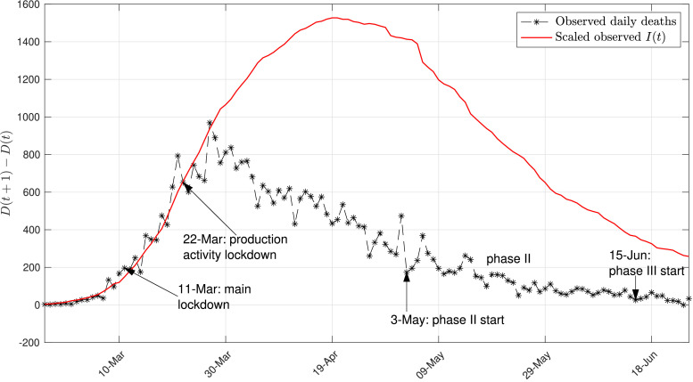
Fig. 1 shows a plot of the daily deaths (national data for Italy) with black dashed line, and the scaled number of active infected individuals with solid red line. The scaling is performed in order to show the approximate proportionality between the daily deaths and the number of active infected, in the early stage of the contagion. This figure also highlight the key dates at which containment measures have been enforced or released.

Fig. 1.

Overall evolution of the COVID-19 contagion in Italy. Daily deaths and scaled number of active infected individuals (national data for Italy). The $I\left(t\right)$ scaling factor is 0.014.

5.1.1. Constant parameter models

In this section, we use the technique illustrated in Section 3.1 for identifying models for the COVID-19 contagion in Italy, assuming constant parameters in the model. Two different models are determined, by fitting the parameters using data from two different time intervals.

Early stage model: Data from February 24th to March 27th of the COVID-19 spread in Italy have been used to fit a model of its early stage using the procedure detailed in Section 3.1. The date of March 27th corresponds to 15 days after the full national lockdown; it is the date at which the containment measures begin to become visible in the data.

Fig. 2 depicts the value attained by the objective function ${\min }_{\theta \ge 0}f(q,\theta )$ for different values of the parameter $q$ in the range $[q_{\min },1]$.

Fig. 2.

Objective cost as a function of $q$ in the early stage model.

The optimal parameter values obtained using the procedure given in Section 3.1 with $q_{\min }=0.0014$ and forgetting factor $w=0.9$ are

$$q=0.011,\beta =0.123,\gamma =0.018,\nu =0.014.$$

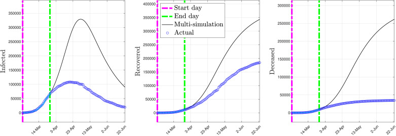
Fig. 3 depicts the multi-simulation prediction — carried out as detailed in Section 4.2 — obtained by using the identified early stage model with the parameters given above. Model identification was carried out using the data corresponding to the time interval from “Start day” to “End day”.

Fig. 3.

Multi-simulation prediction with the early stage model (constant parameters).

As shown by Fig. 3, the early stage model overestimates in the prediction the number of infected, recovered, and deceased individuals. This is essentially due to the fact that such a model does not account for the control measures that have been taken to reduce the spread of COVID-19, such as lockdown, social distancing, etc., since it has been trained only using the early-stage data.

Late stage model: The data from March 27th to May 18th of the COVID-19 spread in Italy have been used to fit a model of its late stage, including the lockdown period, using the procedure detailed in Section 3.1. The optimal parameter values obtained by using the procedure given in Section 3.1 with $q_{\min }=0.0037$ and forgetting factor $w=0.7$ are

$$q=0.014,\beta =0.012,\gamma =0.038,\nu =0.002.$$

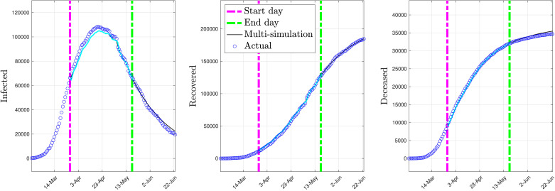
Fig. 4 depicts the multi-simulation prediction — carried out as detailed in Section 4.2 — obtained by using the identified late stage model with the parameters given above.

Fig. 4.

Multi-simulation prediction with the late stage model (constant parameters).

As shown by Fig. 4, the late stage model is capable of predicting the evolution of the post lockdown spread of COVID-19 for a prediction period of 36 days forward with remarkable accuracy.

On the other hand, using a single model with constant parameters for the whole period from February 24th to May 18th presents degraded prediction performance. In fact, the procedure detailed in Section 3.1 has been used to fit a model on these data. The optimal parameter values obtained using the procedure given in Section 3.1 with forgetting factor $w=0.9$ are

$$q=0.0137,\beta =0.0142,\gamma =0.0302,\nu =0.0025.$$

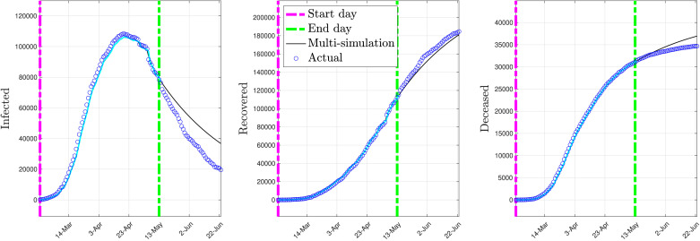
Fig. 5 depicts the multi-simulation prediction — carried out as detailed in Section 4.2 — obtained using the identified model.

Fig. 5.

Multi-simulation prediction with the full data model (constant parameters).

As shown by Fig. 5, the model with constant parameters, fitted over the whole period, shows somewhat degraded prediction performance in the number of infected individuals.

5.1.2. Time-varying parameters models

Motivated by the prediction performance of the model with constant parameters over the whole period from February 24th to May 18th, the main goal of this section is to show that, rather than using two models with constant parameters, it is possible to design a single model with time-varying parameters that is capable of representing the overall evolution of the contagion. A possible design approach is to use the logistic basis functions described at the beginning of Section 4, which essentially lead to piece-wise constant values of the model parameters with smooth transitions. However, the fitting performance with such shape functions resulted to be poorer than the one obtained by using alternative exponential and polynomial basis functions described below. Therefore, the functional form of the basis functions $B\left(t\right),$ $G\left(t\right),$ and $M\left(t\right)$ has been selected as a mixture of negative exponentials and polynomial functions, namely

$$\begin{array}{ccc}\hfill B\left(t\right)& =\hfill & \left[\begin{array}{cccccc}1& {\displaystyle \exp (-\frac{t}{10})}& {\displaystyle \exp (-\frac{t}{11.0526})}& {\displaystyle \exp (-\frac{t}{12.1053})}& {\displaystyle \cdots }& {\displaystyle \exp (-\frac{t}{30})}\end{array}\right],\hfill \\ \hfill {\displaystyle G\left(t\right)}& =\hfill & {\displaystyle \left[\begin{array}{ccc}1& t& {\displaystyle t^2}\end{array}\right],}\hfill \\ \hfill {\displaystyle M\left(t\right)}& =\hfill & {\displaystyle \left[\begin{array}{cccccc}1& {\displaystyle \exp (-\frac{t}{10})}& {\displaystyle \exp (-\frac{t}{11.0526})}& {\displaystyle \exp (-\frac{t}{12.1053})}& \cdots & {\displaystyle \exp (-\frac{t}{30})}\end{array}\right].}\hfill \end{array}$$

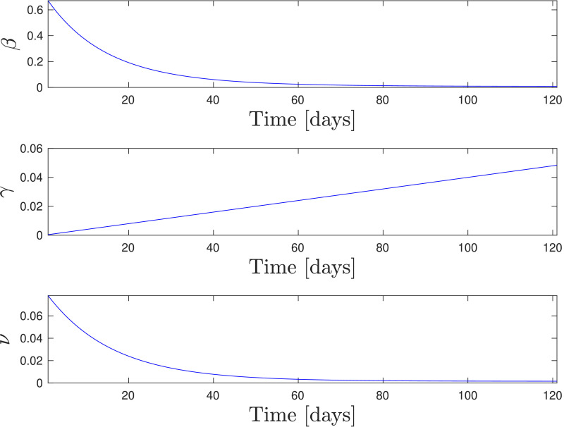
Then, the procedure outlined in Section 4.1.1 has been used to determine the 45 entries of the vector $\mathit{\theta }$ and the parameter $q$ so to fit the model to data. The tradeoff parameter $\lambda$ in the Lasso has been fixed to $\lambda =10,$ leading to ${\parallel \mathit{\theta }\parallel }_0=26,$ and the parameter shapes in Fig. 6 have been obtained. Inspecting the values attained by the parameter $\varrho \left(t\right)=\beta \left(t\right)/\left(\beta \right(t)-\gamma (t)-\nu (t\left)\right),$ we obtained that $\varrho \left(t\right)>0$ for $t\le 58$ and $\varrho \left(t\right)<0$ for $t\ge 59,$ with $t=59$ corresponding to April 22nd. The model then captures the transition from the expansive phase to the controlled phase on the contagion, and predicts a nonzero steady-state value for $\tilde{S}$.

Fig. 6.

Identified shape of the parameters for national data. Time is expressed in days since Feb. 24, 2020.

Further, observe that the time behavior of the fitted parameters shown in Fig. 6 is consistent with their expected dynamics. In fact, the infection rate $\beta$ is expected to decrease thanks to the employment of personal protection equipment, social distancing, improved personal hygiene, and to the detection and isolation of positive individuals. On the other hand, the recovery rate $\gamma$ and the death rate $\nu$ are expected to increase and decrease, respectively, thanks to the use of more effective treatments for the disease.

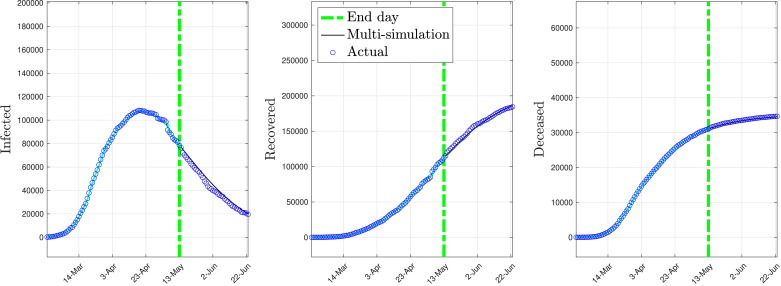
Fig. 7 depicts the multi-simulation prediction — carried out as detailed in Section 4.2 — obtained by using the identified time-varying model with the parameters given above.

Fig. 7.

Multi-simulation prediction with the time-varying model (national data).

As shown by Fig. 7, a single time-varying model suffices to fit the COVID-19 contagion data in Italy both in its early stage and in its late stage. Furthermore, the time-varying model is capable of predicting the evolution of the post lockdown spread of COVID-19 for a prediction period of 41 days forward with remarkable accuracy.

5.2. Analysis of regional data

In this section, the analysis carried out in the previous section considering Italy as a single region is replicated with a focus on each of the four most affected regions in Italy, that is Lombardia, Piemonte, Emilia-Romagna, and Veneto. The same basis functions considered in the previous section have been used to fit a model for each region, using the regional data of COVID-19 spread from February 24th to May 13th.

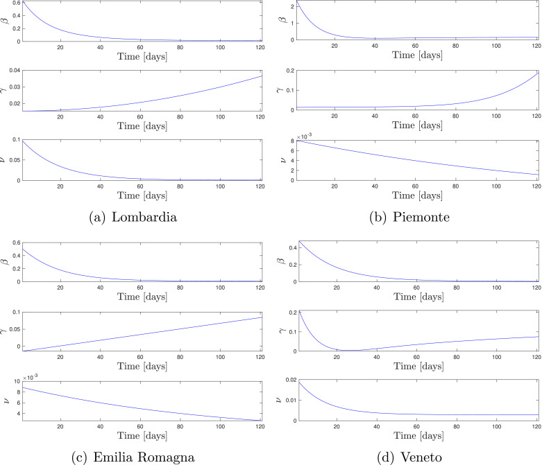
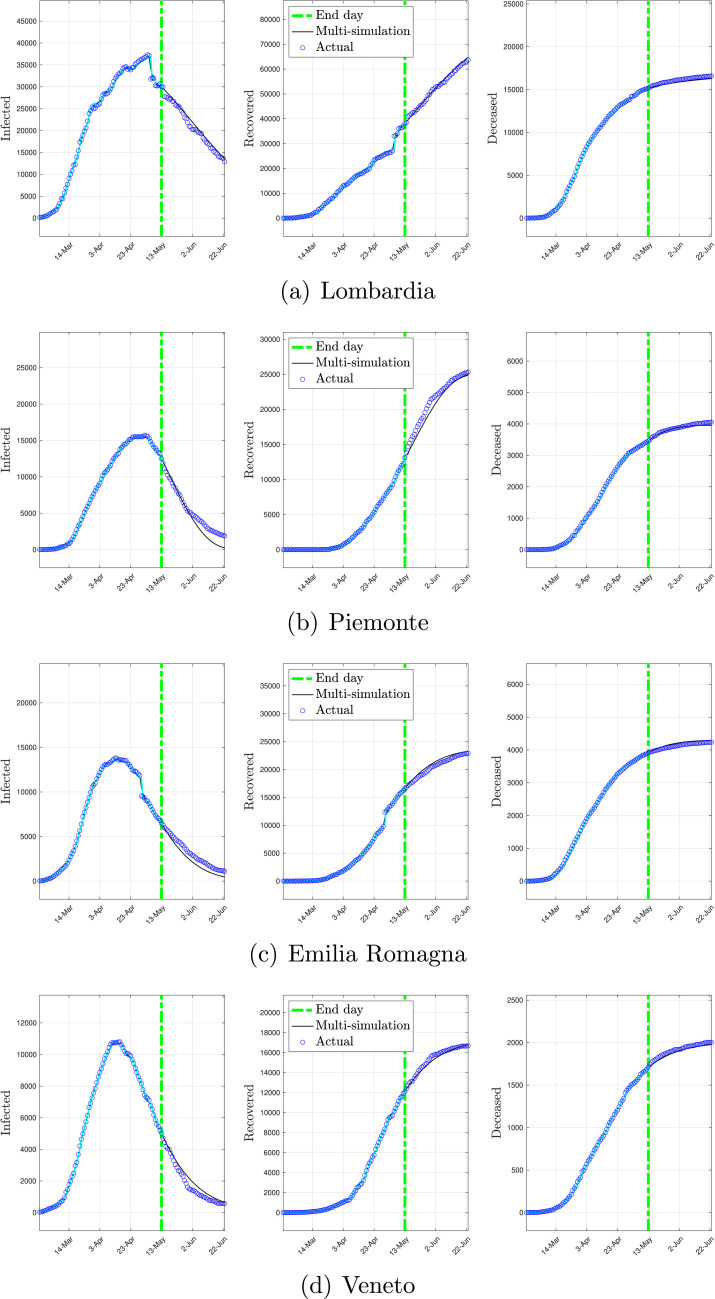
Fig. 8 depicts the parameter shapes identified using regional data and Fig. 9 shows the multi-simulation prediction — carried out as detailed in Section 4.2 — obtained by using the identified time-varying models.

Fig. 8.

Identified shape of the parameters for regional data. Time is expressed in days since Feb. 24, 2020.

Fig. 9.

Multi-simulation prediction with the time-varying model for regional data.

As shown by Fig. 8, the time behavior of the parameters for the regional models is qualitatively similar to the ones obtained from the national model. The only main difference between these behaviors is the non-monotone evolution of the recovery rate $\gamma \left(t\right)$ in the Veneto region, which presents a minimum at March 21st. This might be linked with the stress over intensive care units at the end of March. However, such interpretations shall be taken with care, since specific behaviors might as well be just artifacts of the numerical identification procedure. By observing the time behaviors of the parameters, we can also identify the instants at which the contagion passes from the expansive phase ($\varrho \left(t\right)>0$) to the controlled phase ($\varrho \left(t\right)<0$), which resulted to be May 1st in Lombardia, April 27th in Piemonte, April 16th in Emilia-Romagna, and April 16th in Veneto.

Fig. 9 finally shows that the proposed time-varying model has quite good prediction capabilities in all regions.

6. Discussion

In this paper, a parameter-varying modification of the SIRD model has been proposed for describing and predicting the behavior of the COVID-19 contagion in Italy. Identifying the parameters of this model is a non-trivial non-convex problem, for the solution of which we proposed an approach based on two nested steps: a grid search in the outer loop, and a Lasso optimization problem in the inner step. This approach has been applied to modeling of the COVID-19 contagion in Italy, considering both aggregated national data and regional data from the most affected regions in Italy. In all the considered cases (national and regional), the identified parameter-varying models resulted effective in fitting the COVID-19 contagion data, both in the early and late stages, and in providing accurate predictions of the evolution of the post lockdown epidemic behavior over a forward period of 41 days. Besides these results, the proposed identification approach allows us to have a more detailed understanding of the contagion mechanism with respect to standard time-invariant methods. Indeed, a first important conclusion that can be drawn from Figs. 6 and 8, is that the control measures imposed by the authorities seem to have been effective in reducing the key transmission rate parameter $\beta$. Another interesting observation is that the decrease of this parameter mainly occurs in the first 40 days of the epidemics, and the corresponding trend-inversion of the contagion is observed in the data with a delay of about 15 days, see Figs. 7and 9. Furthermore, a comparison of the different situations in the four considered regions can be made by looking at Figs. 8 and 9. It can be seen that the epidemics decrease is at a more advanced stage in Veneto, Emilia Romagna and Piemonte, whereas Lombardia is still characterized by a relatively high number of infected.

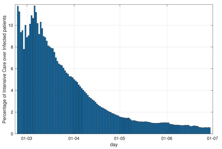
Figs. 6 and 8 show also that the recovery rate tends to increase with time, and the death rate to decrease: this phenomenon, which seems not directly related to the lockdown, can be attributed to different causes, among which a better understanding of the disease and consequent improvement in the effectiveness of the response from the national health system, and possibly a change in the nature, virulence and lethality of the virus. This phenomenon can also be observed directly from the raw data, considering the ratio between the number of individuals that needed Intensive Care in a given day, and the total number of active infected individuals in the same day, see Fig. 10 . This ratio decreased from an initial figure of above 10% in the early stages of the infection to a figure below 1% in the later stages of the infection, showing that the clinical effects of the contagion have reduced greatly with time.

Fig. 10.

Ratio between Intensive Care and Infected individuals (national data).

In conclusion, the proposed COVID-19 modeling approach can be helpful for obtaining epidemic models that are able to describe different phases of the contagion. These models can give reliable short and long term predictions, and also provide useful insight about the contagion mechanisms. Given their time-varying structure, these models could also be effective for simulating different epidemic scenarios, testing various hypotheses, and also for designing suitable control measures by considering the time-varying parameters in the role of control inputs.

Declaration of Competing Interest

The authors declare that they have no known competing financial interests or personal relationships that could have appeared to influence the work reported in this paper.

References

- Bailey N.T.J. 2nd ed. Hafner Press; New York, NY, USA: 1975. The mathematical theory of infectious diseases and its applications. [Google Scholar]
- Brauer F. Mathematical epidemiology: Past, present, and future. Infectious Disease Modelling. 2017;2(2):113–127. doi: 10.1016/j.idm.2017.02.001. [DOI] [PMC free article] [PubMed] [Google Scholar]
- Caccavo, D. (2020). Chinese and italian COVID-19 outbreaks can be correctly described by a modified SIRD model. medRxiv.
- Casella, F. (2020). Can the COVID-19 epidemic be managed on the basis of daily data?arXiv preprint arXiv:2003.06967.
- Chowell G. Fitting dynamic models to epidemic outbreaks with quantified uncertainty: A primer for parameter uncertainty, identifiability, and forecasts. Infectious Disease Modelling. 2017;2(3):379–398. doi: 10.1016/j.idm.2017.08.001. [DOI] [PMC free article] [PubMed] [Google Scholar]
- Chowell G., Tariq A., Hyman J.M. A novel sub-epidemic modeling framework for short-term forecasting epidemic waves. BMC Medicine. 2019;17(1):164. doi: 10.1186/s12916-019-1406-6. [DOI] [PMC free article] [PubMed] [Google Scholar]
- Della Rossa F., Salzano D., Di Meglio A., De Lellis F., Coraggio M., Calabrese C., Guarino A., Cardona-Rivera R., De Lellis P., Liuzza D., Lo Iudice F., Russo G., di Bernardo M. A network model of Italy shows that intermittent regional strategies can alleviate the COVID-19 epidemic. Nature Communications. 2020;11 doi: 10.1038/s41467-020-18827-5. [DOI] [PMC free article] [PubMed] [Google Scholar]
- Di Bernardo M., Russo G., Liuzza D., Della Rossa F., De Lellis P., Lo Iudice F. IEEE-CSS Online Workshop on Modeling and Prediction of Covid-19. 2020. Network model of the covid-19 epidemic in Italy to design and investigate possible containment and mitigation strategies. [Google Scholar]; http://www.ieeecss.it/events/covid.html
- Di Giamberardino P., Iacoviello D. Optimal control of SIR epidemic model with state dependent switching cost index. Biomedical Signal Processing and Control. 2017;31:377–380. [Google Scholar]
- Fernández-Villaverde J., Jones C.I. Technical Report. National Bureau of Economic Research; 2020. Estimating and simulating a SIRD model of COVID-19 for many countries, states, and Cities. [DOI] [PMC free article] [PubMed] [Google Scholar]
- Franco, E. (2020). A feedback SIR (fSIR) model highlights advantages and limitations of infection-based social distancing. arXiv preprint arXiv:2004.13216.
- Garibaldi P., Moen E.R., Pissarides C.A. COVID economics vetted and real-time papers. CEPR; 2020. Modelling contacts and transitions in the SIR epidemics model. [Google Scholar]
- Calafiore G.C., Ghaoui L.E., Novara C. Sparse identification of posynomial models. Automatica. 2015;59:27–34. [Google Scholar]
- Giordano G., Blanchini F., Bruno R., Colaneri P., Di Filippo A., Di Matteo A., Colaneri M. Modelling the COVID-19 epidemic and implementation of population-wide interventions in italy. Nature Medicine. 2020:1–6. doi: 10.1038/s41591-020-0883-7. [DOI] [PMC free article] [PubMed] [Google Scholar]
- Keeling M.J., Eames K.T. Networks and epidemic models. Journal of the Royal Society Interface. 2005;2(4):295–307. doi: 10.1098/rsif.2005.0051. [DOI] [PMC free article] [PubMed] [Google Scholar]
- Kermack W., McKendrick A. A contribution to the mathematical theory of epidemics. Proceedings of the Royal Society of London. 1927;A 115:700–721. doi: 10.1098/rspa.1927.0118. [DOI] [Google Scholar]
- Bohner M., Streipert S., Torres D.F.M. Technical Report. 2018. Exact solution to a dynamic SIR model. [Google Scholar]
- Mizumoto K., Kagaya K., Zarebski A., Chowell G. Estimating the asymptomatic proportion of coronavirus disease 2019 (COVID-19) cases on board the Diamond Princess cruise ship, Yokohama, Japan, 2020. Eurosurveillance. 2020;25(10):2000180. doi: 10.2807/1560-7917.ES.2020.25.10.2000180. [DOI] [PMC free article] [PubMed] [Google Scholar]
- Nadini M., Rizzo A., Porfiri M. Epidemic spreading in temporal and adaptive networks with static backbone. IEEE Transactions on Network Science and Engineering. 2020;7(1):549–561. [Google Scholar]
- Nowzari C., Preciado V.M., Pappas G.J. Optimal resource allocation for control of networked epidemic models. IEEE Transactions on Control of Network Systems. 2015;4(2):159–169. [Google Scholar]
- Pastor-Satorras R., Castellano C., Van Mieghem P., Vespignani A. Epidemic processes in complex networks. Reviews of Modern Physics. 2015;87(3):925. [Google Scholar]
- Pastore Piontti A.Y., Gomes M.F.D.C., Samay N., Perra N., Vespignani A. The infection tree of global epidemics. Network Science. 2014;2(1):132–137. doi: 10.1017/nws.2014.5. [DOI] [Google Scholar]
- Pellis L., Ball F., Bansal S., Eames K., House T., Isham V., Trapman P. Eight challenges for network epidemic models. Epidemics. 2015;10:58–62. doi: 10.1016/j.epidem.2014.07.003. [DOI] [PubMed] [Google Scholar]
- Richards F.J. A flexible growth function for empirical use. Journal of Experimental Botany. 1959;10(2):290–301. doi: 10.1093/jxb/10.2.290. [DOI] [Google Scholar]
- Wertheim J.O., Leigh Brown A.J., Hepler N.L., Mehta S.R., Richman D.D., Smith D.M., Kosakovsky Pond S.L. The global transmission network of HIV-1. Journal of Infectious Diseases. 2014;209(2):304–313. doi: 10.1093/infdis/jit524. [DOI] [PMC free article] [PubMed] [Google Scholar]
- Zino L., Parino F., Porfiri M., Rizzo A. IEEE-CSS Online Workshop on Modeling and Prediction of Covid-19. 2020. A metapopulation activity-driven network model for covid-19 in Italy. [Google Scholar]; http://www.ieeecss.it/events/covid.html