CoxPhLb: An R Package for Analyzing Length Biased Data under Cox Model

Abstract

Data subject to length-biased sampling are frequently encountered in various applications including prevalent cohort studies and are considered as a special case of left-truncated data under the stationarity assumption. Many semiparametric regression methods have been proposed for length-biased data to model the association between covariates and the survival outcome of interest. In this paper, we present a brief review of the statistical methodologies established for the analysis of length-biased data under the Cox model, which is the most commonly adopted semiparametric model, and introduce an R package CoxPhLb that implements these methods. Specifically, the package includes features such as fitting the Cox model to explore covariate effects on survival times and checking the proportional hazards model assumptions and the stationarity assumption. We illustrate usage of the package with a simulated data example and a real dataset, the Channing House data, which are publicly available.

1. Introduction

In prevalent cohort studies, subjects who have experienced an initiating event (e.g., disease diagnosis) but have not yet experienced a failure event (e.g., death) are sampled from the target population and followed until a failure or censoring event occurs. Data collected from such sampling designs are subject to left truncation since subjects who experienced a failure event prior to study enrollment are selectively excluded and are not observed in the data. When the occurrence of the initiating event follows a stationary Poisson process, the data are called “length-biased data”, which is a special case of left-truncated data. These data are encountered in a variety of fields such as cancer screening trials (Zelen and Feinleib, 1969), studies of unemployment (Lancaster, 1979; de Una-Alvarez et al., 2003), epidemiologic cohort studies (Gail and Benichou, 2000; Scheike and Keiding, 2006), and genome-wide linkage studies (Terwilliger et al., 1997). The failure times observed in such data tend to be longer than those in the target population since subjects with longer failure times are more likely to be included in the length-biased data. Figure 1 depicts the occurrence of length-biased sampling. The underlying length-biased sampling assumption (i.e., the stationarity assumption) can be analytically examined (Addona and Wolfson, 2006).

Figure 1:

Illustration of length-biased sampling. Black horizontal lines represent observations that are included in the observed data cohort; gray horizontal lines represent observations excluded; black squares (■) represent uncensored failure events; and empty squares (□) represent censored failure events.

Provided that the observed data are not random samples of the target population, statistical methods for conventional survival data cannot be directly applied to length-biased data. Extensive studies have been conducted on statistical methodologies that account for length bias. In particular, a number of semiparametric regression methods have been proposed in the literature to model the association between covariates and the survival outcome of interest. Among the semiparametric regression models, the Cox proportional hazards model (Cox, 1972) has been the most commonly adopted. Under the Cox model, Wang (1996) proposed a pseudo-partial likelihood approach to assess the covariate effects. However, her estimation method is limited to length-biased data with no right censoring. Tsai (2009) generalized the method to handle potential right censoring. Qin and Shen (2010) constructed estimating equations based on risk sets that are adjusted for length-biased sampling through inverse weights. A thorough review of the existing nonparametric and semiparametric regression methods can be found in Shen et al. (2017).

Although there is a substantial amount of literature on statistical methods for length-biased data, publicly available computational tools for analyzing such data are limited. In this paper, we introduce a new package, CoxPhLb (Lee et al., 2019a), in R that provides tools to analyze length-biased data under the Cox model. The package includes functions that fit the Cox model using the estimation method proposed by Qin and Shen (2010), check the proportional hazards model assumptions based on methods developed by Lee et al. (2019b) and check the underlying stationarity assumption. CoxPhLb is available from the Comprehensive R Archive Network (CRAN) at http://CRAN.R-project.org/package=CoxPhLb. To the best of our knowledge, this is the first and only publicly available R package for analyzing length-biased data under the Cox model.

The remainder of this paper is organized as follows. The following section provides a brief review of the semiparametric estimation method under the Cox model to assess the covariate effects on the survival outcome. Then, we outline how the Cox proportional hazards model assumptions can be checked both graphically and analytically, and describe two approaches to test the stationarity of the underlying incidence process. We illustrate the R package CoxPhLb using a simulated data example and a real dataset, the Channing House data. Finally, we conclude this paper with summarizing remarks.

2. Fitting the Cox model

2.1. Notation and model

Let $\tilde{T}$, $\tilde{A}$, and Z be the duration from an initiating event to failure, the duration from the initiating event to enrollment in the study, and the p × 1 baseline covariate vector, respectively. Assume that the failure time $\tilde{T}$ follows the Cox model,

$$\lambda (t\mid z)={\lambda }_0(t)\text{exp}\left({\beta }_0^{\mathsf{T}}z\right),$$ (1)

where β₀ is a p × 1 vector of unknown regression coefficients and λ₀(t) is an unspecified baseline hazard function. Under length-biased sampling, we only observe failure times that satisfy $\tilde{A}<\tilde{T}$. We denote the length-biased failure time by T = A + V, where A is the observed truncation variable (i.e., backward recurrence time) and V is the duration from study enrollment to failure (i.e., residual survival time or forward recurrence time). Since V is subject to right censoring, the observed failure time is Y = min(T, A + C) and the censoring indicator is δ = I(T ≤ A + C), where C is the duration from study enrollment to censoring (i.e., residual censoring). The data structure is illustrated in Figure 2. We assume that C is independent of A and V given Z, and the distribution of C is independent of Z.

Figure 2:

A diagram of the right-censored length-biased data.

The length-biased data consist of {(Y_i, A_i, δ_i, Z_i), i = 1, … , n}, for n independent subjects. We note that the observed data are not representative of the target population, and the observed biased data do not follow Model (1). Thus, conventional Cox regression methods cannot be used when evaluating the covariate effects on the duration from the initiating event to failure for the target population. Furthermore, even under the independent censoring assumption on C with A and V, the sampling mechanism induces dependent censoring because Cov(T, A + C ∣ Z) = Var(A ∣ Z) + Cov(A, V ∣ Z) > 0.

2.2. Estimation of the covariate effects

Among many estimation methods established for length-biased data under the Cox model, we provide the estimation function based on the inversely weighted estimating equation of Qin and Shen (2010). While this estimating equation approach may not be the most efficient method, the estimation procedure is easy to implement and provides a mean zero stochastic process that forms the basis of model checking. We adopt this estimation method for model fitting and checking in the R package CoxPhLb.

For subject i, we denote N_i(t) = I{Y_i ≤ t, δ_i = 1} and R_i(t) = I{Y_i ≥ t, δ_i = 1} following the counting process notation. Let a⁰ = 1, a¹ = a, and a² = aa⊺ for any vector a. Define

$$S^{(k)}(\beta ,t)=n^{-1}\sum _{i=1}^n{w}_C(t)R_i(t)\{w_C(Y_i){\}}^{-1}{\mathit{Z}}_i^k\text{exp}({\beta }^{\mathsf{T}}{\mathit{Z}}_i),$$

where the weight function $w_C(y)={\int }_0^y{S}_C(u)\mathrm{d}u$, in which S_C(y) = Pr(C > y) is the survival function of the residual censoring variable C for k = 0, 1, and 2. By replacing w_C(y) with its consistent estimator, ${\widehat{w}}_C(y)={\int }_0^y{\widehat{S}}_C(u)\mathrm{d}u$, where ${\widehat{S}}_C(\cdot )$ is the Kaplan–Meier estimator of the residual censoring survival function, we have

$${\widehat{S}}^{(k)}(\beta ,t)=n^{-1}\sum _{i=1}^n{\widehat{w}}_C(t)R_i(t)\{{\widehat{w}}_C(Y_i){\}}^{-1}{\mathit{Z}}_i^k\text{exp}({\beta }^{\mathsf{T}}{\mathit{Z}}_i)$$

for k = 0, 1, and 2. The regression parameter β₀ can be estimated by solving the following unbiased estimating equation:

$$\widehat{U}(\beta )=\sum _{i=1}^n{\int }_0^{\tau }\left\{{\mathit{Z}}_i-\widehat{E}(\beta ,u)\right\}\mathrm{d}{N}_i(u)=0,$$ (2)

where τ satisfies Pr(Y ≥ τ) > 0 and $\widehat{E}(\beta ,t)={\widehat{S}}^{(1)}(\beta ,t)∕{\widehat{S}}^{(0)}(\beta ,t)$. The solution to Equation (2), which is denoted by $\widehat{\beta }$, is unique and a consistent estimator to β₀. Using the Taylor series expansion, it can be shown that the distribution of $\widehat{\beta }$ converges weakly to a normal distribution with variance Γ⁻¹ΣΓ⁻¹, where $\Gamma =-{\text{lim}}_{n\to \infty }{n}^{-1}\partial \widehat{U}(\beta )∕\partial \beta$ and Σ is the covariance matrix of ${\text{lim}}_{n\to \infty }{n}^{-1∕2}\widehat{U}({\beta }_0)$.

This estimation procedure can be implemented using the coxphlb function in the CoxPhLb package as follows:

coxphlb(formula, data, method = c("Bootstrap","EE"), boot.iter = 500,
    seed.n = round(runif(1,1,1e09)), digits = 3L)

where formula has the same syntax as the formula used in coxph from the survival package (Therneau, 2020). The response needs to be a survival object such as Surv(a, y, delta) where a, y, and delta are the truncation times, the observed failure times, and the censoring indicators, respectively. The argument data is a data frame that includes variables named in the formula. We can choose either the bootstrap variance estimates ("Bootstrap"), or the model-based variance estimates ("EE") to be returned in the fitted model object through the argument method. When bootstrap resampling is chosen for variance estimation, the bootstrap sample size is controlled by boot.iter with the default set as 500, and a seed number can be fixed by seed.n. A summary table is returned with values rounded by the integer set through digits.

Alternatively, one can implement the estimation procedure by using the coxph function with the subset of the data that consist of uncensored failure times only and an offset term to add $\log \{{\widehat{w}}_C(Y_i){\}}^{-1}$ to the linear predictor with a fixed coefficient of one as discussed in Qin and Shen (2010). The coxph function will return the same point estimates as the coxphlb function. To compute the corresponding standard errors using coxph, we need to use the bootstrap approach. Later, in the simulated data example, we further evaluate the computational efficiency of the coxphlb function with the model-based variance estimation (i.e., method = EE) opposed to the bootstrap resampling method (i.e., method = Bootstrap).

3. Checking the Cox model assumptions

Two primary components of checking the Cox proportional hazards model assumptions are examining (i) the functional form of a covariate and (ii) the proportional hazards assumption. To detect violations of these model assumptions, the general form of the cumulative sums of multiparametric stochastic processes is considered.

Under Model (1), we can construct a mean zero stochastic process,

$$M_i(t)=N_i(t)-{\int }_0^t{w}_C(u)R_i(u)\{w_C(Y_i){\}}^{-1}\text{exp}({\beta }_0^{\mathsf{T}}{\mathit{Z}}_i)\mathrm{d}{\Lambda }_0(u),$$

for i = 1, … , n, where ${\Lambda }_0(t)={\int }_0^t{\lambda }_0(s)\mathrm{d}s$ is the cumulative baseline hazard function. The stochastic process can be estimated by

$${\widehat{M}}_i(t)=N_i(t)-{\int }_0^t{\widehat{w}}_C(u)R_i(u)\{{\widehat{w}}_C(Y_i){\}}^{-1}\text{exp}({\widehat{\beta }}^{\mathsf{T}}{\mathit{Z}}_i)\mathrm{d}{\widehat{\Lambda }}_0(\widehat{\beta },u),$$

where

$${\widehat{\Lambda }}_0(\widehat{\beta },t)={\int }_0^t\frac{{\sum }_{i=1}^n\mathrm{d}{N}_i(u)}{n{\widehat{S}}^{(0)}(\widehat{\beta },u)}.$$

The stochastic process can be considered as the difference between the observed and the expected number of events, which mimics the ordinary martingale residuals. When the estimated processes ${\widehat{M}}_i(t)$, i = 1, … , n deviate from zero systematically, it may be a sign of model misspecification.

Let

$$\mathit{G}(t,z)=\sum _{i=1}^{n}f({\mathit{Z}}_i)I({\mathit{Z}}_i\le \mathit{z}){\widehat{M}}_i(t),$$ (3)

where f(·) is a prespecified smooth and bounded function, and I(Z_i ≤ z) = I(Z_i1 ≤ z₁, … , Z_ip ≤ z_p) with Z_i = (Z_i1, … , Z_ip)^⊺ and z = (z₁, … , z_p)^⊺. When the model assumptions are satisfied, the process (3) will fluctuate randomly around zero. We can adjust the general form (3) to examine the specific model assumptions. To assess the functional form of the jth covariate, we choose f(·) = 1, t = τ, and z_k = ∞ for all k ≠ j. The proportional hazards assumption for the jth covariate can be evaluated by setting f(Z_ij) = Z_ij and z = ∞. To develop analytical test procedures, test statistics can be constructed using the supremum test, sup_t,z∣G(t,z)∣. Let $T_1^j={\text{sup}}_z\mid {\mathit{G}}_1^j(z)\mid$ be the test statistics for checking the functional form of the jth covariate, where ${\mathit{G}}_1^j(z)={\sum }_{i=1}^{n}I(Z_{ij}\le z){\widehat{M}}_i(\tau )$; and $T_2^j={\text{sup}}_t\mid {\mathit{G}}_2^j(t)\mid$, where ${\mathit{G}}_2^j(t)={\sum }_{i=1}^n{Z}_{ij}{\widehat{M}}_i(t)$ for checking the proportional hazards assumption for the jth covariate. We can also consider the global test statistic $T_2={\text{sup}}_t{\sum }_{j=1}^p\mid {\mathit{G}}_2^j(t)\mid$ when the overall proportionality of hazards for all covariates is of interest.

The null distribution of the general form (3) under Model (1) has been studied in Lee et al. (2019b) to derive the critical values for test statistics $T_1^j$, $T_2^j$, and T₂. We can approximate the null distribution by adopting the resampling technique used in Lin et al. (1993). Let

$$\begin{gathered} {\widehat{\mathit{G}}}_i^{\ast }(t,\mathit{z})={\int }_0^t\left\{f({\mathit{Z}}_i)I({\mathit{Z}}_i\le \mathit{z})-{\widehat{E}}_Z(\widehat{\beta },u,\mathit{z})\right\}\mathrm{d}{\widehat{M}}_i(u)+{\int }_0^t\widehat{H}(\widehat{\beta },u)\frac{\mathrm{d}{\widehat{M}}_{C_i}(u)}{\widehat{\pi }(u)} \\ +{\widehat{\Gamma }}_Z(\widehat{\beta },t,\mathit{z})\{\widehat{\Gamma }(\widehat{\beta }){\}}^{-1}{\int }_0^{\tau }\left\{{\mathit{Z}}_i-\widehat{E}(\widehat{\beta },u)\right\}\mathrm{d}{\widehat{M}}_i(u), \end{gathered}$$

Where

$${\widehat{S}}_Z^{(l)}(\beta ,t,\mathit{z})=n^{-1}\sum _{i=1}^{n}f({\mathit{Z}}_i)I({\mathit{Z}}_i\le \mathit{z}){\widehat{w}}_C(t)R_i(t)\{{\widehat{w}}_C(Y_i){\}}^{-1}{\mathit{Z}}_i^l\text{exp}({\beta }^{\mathsf{T}}{\mathit{Z}}_i)$$

for l = 0; 1, ${\widehat{E}}_Z(\beta ,u,\mathit{z})={\widehat{S}}_Z^{(0)}(\beta ,t,\mathit{z})∕{\widehat{S}}^{(0)}(\beta ,t)$,

$$\begin{gathered} \widehat{H}(\beta ,t)=\sum _{i=1}^n\sum _{k=1}^n\frac{f({\mathit{Z}}_k)I({\mathit{Z}}_k\le z){\widehat{w}}_C(Y_i)R_k(Y_i)\text{exp}({\beta }^{\mathsf{T}}{\mathit{Z}}_k)\{{\widehat{w}}_C(Y_k){\}}^{-2}{\widehat{h}}_k(t)}{n^2{\widehat{S}}^{(0)}(\beta ,Y_i)} \\ ,{\widehat{M}}_{C_i}(t)=I(V_i\le t,{\delta }_i=0)-{\int }_0^{t}I(V_i\ge u)\mathrm{d}{\widehat{\Lambda }}_C(u), \\ {\widehat{h}}_k(t)=I(Y_k\ge t){\int }_t^{Y_k}{\widehat{S}}_C(u)\mathrm{d}u, \\ \widehat{\pi }(t)={\widehat{S}}_C(t){\widehat{S}}_V(t), \end{gathered}$$

in which ${\widehat{\Lambda }}_C(\cdot )$ is the Nelson-Aalen estimator for the residual censoring time and ${\widehat{S}}_V(\cdot )$ is the Kaplan–Meier estimator of the residual survival time, and

$$\begin{gathered} {\widehat{\Gamma }}_Z(\beta ,t,\mathit{z})=n^{-1}\sum _{i=1}^n{\int }_0^t\left[\frac{{\widehat{S}}_{\mathit{Z}}^{(1)}(\beta ,u,\mathit{z})}{{\widehat{S}}^{(0)}(\beta ,u)}-\frac{{\widehat{S}}_{\mathit{Z}}^{(0)}(\beta ,u,\mathit{z}){\widehat{S}}^{(1)}(\beta ,u)}{\{{\widehat{S}}^{(0)}(\beta ,u){\}}^2}\right]\mathrm{d}{N}_i(u), \\ \widehat{\Gamma }(\beta )=-n^{-1}\sum _{i=1}^n{\int }_0^{\tau }\left[\frac{{\widehat{S}}^{(2)}(\beta ,u)}{{\widehat{S}}^{(0)}(\beta ,u)}-{\left\{\frac{{\widehat{S}}^{(1)}(\beta ,u)}{{\widehat{S}}^{(0)}(\beta ,u)}\right\}}^2\right]\mathrm{d}{N}_i(u). \end{gathered}$$

Define ${\tilde{\mathit{G}}}_m(t,\mathit{z})={\sum }_{i=1}^n{\widehat{\mathit{G}}}_i^{\ast }(t,\mathit{z})V_{mi}$, where V_mi, i = 1, … , n, are independent random variables sampled from a standard normal distribution for m = 1, … , M. The simulated realizations of ${\tilde{\mathit{G}}}_m(t,\mathit{z})$ for a large M approximate the null distribution. For graphical assessment, we can plot a few randomly chosen realizations of ${\tilde{\mathit{G}}}_m(t,\mathit{z})$ and compare the observed process based on the data with them. A departure of the observed process from the simulated realizations implies violations of model assumptions. For an analytical test, the critical values for the test statistics can be derived by simulating ${\text{sup}}_{t,z}\mid {\tilde{\mathit{G}}}_m(t,z)\mid$ for m = 1, … , M. We can compute the p values by the proportion of critical values greater than the test statistic.

We can carry out model checking in R using the function coxphlb.ftest to examine the functional form of a continuous covariate as follows:

coxphlb.ftest(fit, data, spec.p = 1, n.sim = 1000, z0 = NULL, seed.n = round(runif(1,1,1e09)),
   digits = 3L)

where the argument fit is an object of the "coxphlb" class, which can be obtained by using the coxphlb function, and data is the data frame used in the fitted model. We specify the jth component of the covariates to be examined via spec.p, where the default is set as j = 1. To approximate the null distribution, we sample a large number of realizations. The argument n.sim controls the number of samples with the default set as 1000. When specific grid points over the support of the jth covariate are to be examined, we can plug them in as a vector in z0, which if NULL, 100 equally distributed grid points will be selected over the range of the jth covariate by default. The random seed number can be fixed through seed.n. The p value returned by the function is rounded by the integer set via digits. To test the proportional hazards assumption, we use coxphlb.phtest as follows:

coxphlb.phtest(fit, data, spec.p = NULL, n.sim = 1000, seed.n = round(runif(1,1,1e09)),
   digits = 3L)

where all arguments play the same role as in the coxphlb.ftest function, except for spec.p. The proportional hazards assumption can be tested for the jth covariate if we set spec.p equal to j. The function will conduct the global test by default if spec.p is left unspecified.

We can conduct graphical assessment by using the following functions:

coxphlb.ftest.plot(x, n.plot = 20, seed.n = round(runif(1,1,1e09)))
coxphlb.phtest.plot(x, n.plot = 20, seed.n = round(runif(1,1,1e09)))

where x are objects of the "coxphlb.ftest" class and the "coxphlb.phtest” class, respectively. These functions return a plot of the observed process along with a randomly sampled n.plot number of realizations. We can fix the random seed number through seed.n.

4. Checking the stationarity assumption

When the underlying incidence process follows a stationary Poisson process, the distribution of the truncation variable is uniform and the data are considered length-biased. In the literature, two approaches have been proposed to check the stationarity assumption: a graphical assessment and an analytical test procedure. Asgharian et al. (2006) demonstrated that the stationarity assumption can be checked graphically by comparing the Kaplan–Meier estimators based on the current and residual survival times. A large discrepancy indicates that the stationarity assumption is invalid. Addona and Wolfson (2006) proposed an analytic test to check the assumption. They showed that testing the stationarity assumption is equivalent to testing whether the distributions of the backward and forward recurrence times are the same. Let F(t) = Pr(A ≤ t) and G(t) = Pr(V* ≤ t, δ = 1), where V* = min(V, C). Following Wei (1980), the test statistic can be constructed as follows:

$$W=n^{-2}\sum _{i=1}^n\sum _{j=1}^n\{\Phi (A_i,V_j^{\ast },{\delta }_j)-p\},$$

where $\Phi (A_i,V_j^{\ast },{\delta }_j)=I(A_i>V_j^{\ast },{\delta }_j=1)-I(A_i<V_j^{\ast })$ and $p=\mathrm{E}\{G(A_i)\}-\mathrm{E}\{F(V_j^{\ast })\}$. The limiting distribution of the test statistic W has been studied in Addona and Wolfson (2006), and the corresponding p value can be computed.

In R, we can explore the stationarity assumption graphically using function station.test.plot as follows:

station.test.plot(a, v, delta)

where a is the vector of backward recurrence times, v is the vector of forward recurrence times, and delta is the vector of censoring indicators. The function produces a plot of two Kaplan–Meier curves. To test the assumption analytically, we can use

station.test(a, v, delta, digits = 3L)

where the data input arguments are the same as those in the station.test.plot function. The test statistic and the corresponding p value based on the two-sided test will be returned with the values rounded by the integer set by digits.

5. Implementation of CoxPhLb

The three major components of CoxPhLb are (i) model fitting using function coxphlb, (ii) model checking using functions coxphlb.ftest and coxphlb.phtest, and (iii) stationarity assumption testing using function station.test. An overview of all functions in the CoxPhLb package is presented in Table 1. In the following sections, we provide R codes that illustrate how to use the functions with the simulated data that are available in the CoxPhLb package and a real dataset, the Channing House data, which is publicly available in the KMsurv package (Klein et al., 2012). The provided R codes can be implemented after installing and loading the CoxPhLb package, which will automatically load the survival package.

Table 1:

Summary of functions in the CoxPhLb package.

Function	Description	S3 methods
coxphlb	Fits a Cox model to right-censored length-biased data	print() summary() coef() vcov()
coxphlb.ftest	Tests the functional form of covariates	print()
coxphlb.phtest	Tests the proportional hazards assumption	print()
station.test	Tests the stationarity assumption	print()
coxphlb.ftest.plot	Returns a graph for testing the functional form of covariates
coxphlb.phtest.plot	Returns a graph for testing the proportional hazards assumption
station.test.plot	Returns a graph for testing the stationarity assumption

5.1. The simulated data example

We use the simulated dataset, ExampleData1, that is available in the CoxPhLb package for illustration. The data have 200 observations and consist of length-biased failure times (y), the truncation variable (a), the censoring indicator (delta), and two covariates, X₁ with binary values (x1) and X₂ with continuous values that range from 0 to 1 (x2). The vector of forward recurrence times (v) is the difference between the failure times and the backward recurrence times (y-a).

We begin by checking the stationarity assumption of the simulated dataset graphically as follows.

> data("ExampleData1", package = "CoxPhLb")
> dat1 <- ExampleData1
> station.test.plot(a = dat1$a, v = dat1$y - dat1$a, delta = dat1$delta)

The resulting plot is presented in Figure 3. We observe that the two Kaplan–Meier curves are very close to each other, especially at the early time points, which provides some evidence of the stationarity of incidence. However, we note some discrepancy in the tails of the curves. Thus, we conduct an analytical test to verify the underlying assumption as follows.

Figure 3:

Testing the stationarity assumption for Example Data 1.

> station.test(a = dat1$a, v = dat1$y - dat1$a, delta = dat1$delta)
  test.statistic p.value
  −0.375 0.707

To save the computed test statistic and the corresponding p value in the form of a list, we may assign the function outputs to an object. The analytical test provides a p value of 0.707, which indicates that the underlying stationarity of the incidence process is reasonable for the simulated dataset. Given that the data are subject to length bias, we evaluate the covariate effects on the failure time under the Cox model using the estimation method for length-biased data. First, we consider the model-based variance estimation.

> fit.eel <- coxphlb(Surv(a, y, delta) ~ x1 + x2, data = dat1, method = "EE")
  Call:
  coxphlb(formula = Surv(a, y, delta) ~ x1 + x2, method = EE)
     coef variance std.err z.score p.value lower.95 upper.95
  x1 1.029 0.031 0.177 5.83 <0.001 0.683 1.375
  x2 0.45 0.132 0.364 1.24 0.216 −0.263 1.163

The outputs include the estimated coefficients, the corresponding variance and the standard error estimates, the computed z scores and p values, and the 95% confidence intervals. In the above example R code, the list of outputs is saved by fit.ee1 as an object of the "coxphlb" class. In the resulting table, we observe that the effect of X₁ is significant whereas that of X₂ is not. As an alternative approach for estimating the variance, we may use the bootstrap resampling method as follows.

> coxphlb(Surv(a, y, delta) ~ x1 + x2, data = dat1, method = "Bootstrap", seed.n = 1234)
  Call:
  coxphlb(formula = Surv(a, y, delta) ~ x1 + x2, method = Bootstrap)
     coef variance std.err z.score p.value lower.95 upper.95
  x1 1.029 0.032 0.178 5.78 <0.001 0.68 1.378
  x2 0.45 0.133 0.365 1.23 0.218 −0.266 1.166

The outputs based on the bootstrap resampling method (i.e., method = Bootstrap) are close to the results from the model-based variance estimation (i.e., method = EE). To measure the average execution times of the two variance estimation methods, we ran the coxphlb function 100 times. The average execution times were 0.972s and 3.581s for method = EE and Bootstrap, respectively, on a desktop computer with Intel Core i5 CPU@3.40GHz and 8 GB 2400 MHz DDR4 of memory, which demonstrates the computational efficiency of coxphlb with the model-based variance estimation.

We note that the estimation results are only valid when the Cox proportional hazards model assumptions are correct. We thus verify the proportional hazards model assumptions. First, the linear functional form of the second covariate which has continuous values, can be checked as follows.

> ftest1 <- coxphlb.ftest(fit = fit.ee1, data = dat1, spec.p = 2, seed.n = 1234)
     p.value
  x2 0.433
> coxphlb.ftest.plot(ftest1, n.plot = 50, seed.n = 1234)

To test the linear functional form, the object fit.ee1 is specified as an input argument. We set spec.p = 2 to conduct the test for X₂ and set seed.n = 1234 for reproducible results. The coxphlb.ftest function returns a p value from the analytical test. For graphical assessment, we specify the object ftest1 which is in the "coxphlb.ftest" class and set n.plot = 50 to plot 50 realization lines. Based on Figure 4 and the p value, the functional form of X₂ satisfies the model assumption. Another important assumption of the Cox model is the proportional hazards assumption. We first test the assumption for each covariate and then conduct the global test for the overall proportionality.

Figure 4:

Checking the functional form of continuous covariate X₂ of Example Data 1.

> phtest11 <- coxphlb.phtest(fit = fit.ee1, data = dat1, spec.p = 1, seed.n = 1234)
     p.value
  x1 0.59
> phtest12 <- coxphlb.phtest(fit = fit.ee1, data = dat1, spec.p = 2, seed.n = 1234)
     p.value
  x2 0.833
> coxphlb.phtest.plot(phtest11, n.plot = 50, seed.n = 1234)
> coxphlb.phtest.plot(phtest12, n.plot = 50, seed.n = 1234)

The outputs consist of the p values derived from the analytical tests of checking the proportional hazards assumption and a plot of the stochastic processes. Figure 5 shows that the proportional hazards assumption is reasonable for both covariates. This is further confirmed by the computed p values, which are greater than 0.05.

Figure 5:

Checking the proportional hazards assumption for covariates X₁ and X₂ of Example Data 1.

> coxphlb.phtest(fit = fit.ee1, data = dat1, spec.p = NULL, seed.n = 1234)
         p.value
GLOBAL 0.762

The global test can be conducted by specifying spec. p = NULL. The result is consistent with the tests performed for each covariate. Note that the graphical assessment is unavailable for the global test.

5.2. The Channing House data

The Channing House data were collected from 462 individuals at a retirement center located in Palo Alto, California, from 1964 to 1975 (Klein and Moeschberger, 2003). We consider the elders aged 65 years or older as the target group of interest. Hence, we analyze the subset of the dataset composed of 450 individuals who entered the center at age 65 or older, in which 95 are males and 355 are females. The data include information of death indicator (death), age at entry (ageentry), age at death or censoring (age), and gender (gender). The observed survival times are left-truncated because only individuals who have lived long enough to enter the retirement center will be included in the data. We load the original dataset and select the subset of the dataset for illustration. Note that we convert age measured in months to years.

> install.packages("KMsurv")
> data("channing", package = "KMsurv")
> dat2 <- as.data.frame(cbind(ageentry = channing$ageentry/12, age = channing$age/12,
+         death = channing$death, gender = channing$gender))
> dat2 <- dat2[dat2$ageentry >=65, ]

First, we check the stationarity assumption as follows.

> station.test.plot(a = (dat2$ageentry - 65), v = (dat2$age - dat2$ageentry),
+    delta = dat2$death)

The resulting plot in Figure 6 provides a strong sign that the stationarity assumption is satisfied. We further verify the assumption by conducting the analytical test.

Figure 6:

Testing the stationarity assumption for Channing House data.

> station.test(a = (dat2$ageentry - 65), v = (dat2$age - dat2$ageentry),
+              delta = dat2$death)
  test.statistic p.value
  0.261 0.794

Based on the results, we can conclude that the stationarity assumption is valid. Hence, we use the functions in CoxPhLb to assess the covariate effects on the survival outcome for the Channing House data. The model can be fitted as follows.

> fit.ee2 <- coxphlb(Surv((ageentry - 65), (age - 65), death) ~ gender, data = dat2,
+      method = "EE")
  Call:
  coxphlb(formula = Surv((ageentry - 65), (age - 65), death) ~ gender, method = EE)
         coef   variance std.err z.score p.value lower.95 upper.95
  gender −0.112 0.029    0.17     −0.66  0.509   −0.445   0.22

Using the model-based variance estimation, we find that gender is not a significant factor for survival. The bootstrap resampling approach provides consistent results as follows.

> coxphlb(Surv((ageentry - 65), (age - 65), death) ~ gender, data = dat2,
+         method = "Bootstrap", seed.n = 1234)
  Call:
  coxphlb(formula = Surv((ageentry - 65), (age - 65), death) ~ gender, method = Bootstrap)
         coef   variance std.err z.score p.value lower.95 upper.95
  gender −0.112 0.028  0.168 −0.67 0.504 −0.441 0.217

The estimation of the covariate effects is only valid when the Cox model assumptions are not violated. By conducting the following proportional hazards assumption test, we verify that the assumption is reasonable based on the computed p value and Figure 7.

Figure 7:

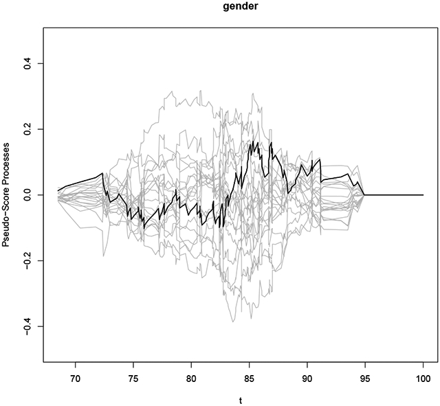
Checking the proportional hazards assumption for gender in the Channing House data.

> phtest2 <- coxphlb.phtest(fit = fit.ee2, data = dat2, spec.p = 1, seed.n = 1234)
         p.value
  gender 0.723
> coxphlb.phtest.plot(phtest2, seed.n = 1234)

6. Summary

Observational data subject to length-biased sampling have been widely recognized by epidemiologists, clinicians, and health service researchers. While statistical methodologies have been well established for analyzing such types of failure time data, the lack of readily available software has been a barrier to the implementation of proper methods. We introduce the R package CoxPhLb that allows practitioners to easily and properly analyze length-biased data under the Cox model, which is commonly used for conventional survival data. When the stationarity assumption is uncertain for the data, one can check the assumption graphically and analytically using tools provided in the package prior to fitting the Cox model. In addition, the fundamental assumptions of the Cox model can be examined.

The CoxPhLb package may be further expanded by including other estimation approaches under the Cox model. For example, Qin et al. (2011) proposed an estimation method based on the full likelihood, which involves more intensive computations. Implementation of this method yields more efficient estimators, which is certainly desirable. In addition, when a violation of the proportional hazards assumption is detected by the coxphlb.phtest or coxphlb.phtest.plot functions, we may consider extending the regression method to handle covariates with non-proportionality such as the coxphw package (Dunkler et al., 2018) which implements the weighted Cox regression method for conventional survival data. We leave these possible extensions for future work.

References

- Addona V and Wolfson DB. A formal test for the stationarity of the incidence rate using data from a prevalent cohort study with follow-up. Lifetime Data Analysis, 12:267–284, 2006. URL 10.1007/s10985-006-9012-2. [DOI] [PubMed] [Google Scholar]
- Asgharian M, Wolfson DB, and Zhang X. Checking stationarity of the incidence rate using prevalent cohort survival data. Statistics in Medicine, 25:1751–1767, 2006. URL 10.1002/sim.2326. [DOI] [PubMed] [Google Scholar]
- Cox DR. Regression models and life-tables (with discussion). Journal of Royal Statistical Society B, 34: 187–220, 1972. URL 10.1111/j.2517-6161.1972.tb00899.x. [DOI] [Google Scholar]
- de Una-Alvarez J, Otero-Giraldez MS, and Alvarez-Llorente G. Estimation under length-bias and rightcensoring: an application to unemployment duration analysis for married women. Journal of Applied Statistics, 30:283–291, 2003. URL 10.1080/0266476022000030066. [DOI] [Google Scholar]
- Dunkler Daniela, Ploner Meinhard, Schemper Michael, and Heinze Georg. Weighted cox regression using the r package coxphw. Journal of Statistical Software, 84:1–26, 2018. URL 10.18637/jss.v084.i02.30450020 [DOI] [Google Scholar]
- Gail MH and Benichou J. Encyclopedia of Epidemiologic Methods. Chichester: Wiley, 2000. [Google Scholar]
- Klein JP and Moeschberger ML. Survival analysis: techniques for censored and truncated data. Springer-Verlag; New York, Inc., 2nd edition, 2003. URL 10.1007/978-1-4757-2728-9. [DOI] [Google Scholar]
- Klein JP, Moeschberger ML, and J. modifications by Yan. KMsurv: Data sets from Klein and Moeschberger (1997), Survival Analysis, 2012. URL https://CRAN.R-project.org/package=KMsurv. R package version 0.1-5. [Google Scholar]
- Lancaster T. Econometric methods for the duration of unemployment. Econometrica, 47:939–956, 1979. URL 10.2307/1914140. [DOI] [Google Scholar]
- Lee CH, Liu DD, Ning J, Zhou H, and Shen Y. CoxPhLb: Analyzing Right-Censored Length-Biased Data, 2019a. URL https://CRAN.R-project.org/package=CoxPhLb. R package version 1.2.0. [Google Scholar]
- Lee CH, Ning J, and Shen Y. Model diagnostics for the proportional hazards model with length-biased data. Lifetime Data Analysis, 25:79–96, 2019b. URL 10.1007/s10985-018-9422-y. [DOI] [PMC free article] [PubMed] [Google Scholar]
- Lin DY, Wei LJ, and Ying ZL. Checking the cox model with cumulative sums of martingale-based residuals. Biometrika, 80:557–572, 1993. URL 10.2307/2337177. [DOI] [Google Scholar]
- Qin J and Shen Y. Statistical methods for analyzing right-censored length-biased data under cox model. Biometrics, 66:382–392, 2010. URL 10.1111/j.1541-0420.2009.01287.x. [DOI] [PMC free article] [PubMed] [Google Scholar]
- Qin J, Ning J, Liu H, and Shen Y. Maximum likelihood estimations and em algorithms with length-biased data. Journal of American Statistical Association, 106:1434–1449, 2011. URL 10.1198/jasa.2011.tm10156. [DOI] [PMC free article] [PubMed] [Google Scholar]
- Scheike TH and Keiding N. Design and analysis of time-to-pregnancy. Statistical Methods in Medical Research, 15:127–140, 2006. URL 10.1191/0962280206sm435oa. [DOI] [PubMed] [Google Scholar]
- Shen Y, Ning J, and Qin J. Nonparametric and semiparametric regression estimation for length-biased survival data. Lifetime Data Analysis, 23:3–24, 2017. URL 10.1007/s10985-016-9367-y. [DOI] [PMC free article] [PubMed] [Google Scholar]
- Terwilliger JD, Shannon WD, Lathrop GM, Nolan JP, Goldin LR, Chase GA, and Weeks DE. True and false positive peaks in genomewide scans: applications of length-biased sampling to linkage mapping. American Journal of Human Genetics, 61:430–438, 1997. URL 10.1086/514855. [DOI] [PMC free article] [PubMed] [Google Scholar]
- Therneau Terry M. A Package for Survival Analysis in R, 2020. .URL https://CRAN.R-project.org/package=survival. R package version 3.1-12. [Google Scholar]
- Tsai WY. Pseudo-partial likelihood for proportional hazards models with biased-sampling data. Biometrika, 96:601–615, 2009. URL 10.1093/biomet/asp026. [DOI] [PMC free article] [PubMed] [Google Scholar]
- Wang MC. Hazards regression analysis for length-biased data. Biometrika, 83:343–354, 1996. URL 10.1093/biomet/83.2.343. [DOI] [Google Scholar]
- Wei LJ. A generalized gehan and gilbert test for paired observations that are subject to arbitrary right censorship. Journal of American Statistical Association, 75:634–637, 1980. URL 10.1080/01621459.1980.10477524. [DOI] [Google Scholar]
- Zelen M and Feinleib M. On the theory of screening for chronic diseases. Biometrika, 56:601–614, 1969. URL 10.1093/biomet/56.3.601. [DOI] [Google Scholar]