Occurrence and Health Risks of Organic Micro-Pollutants and Metals in Groundwater of Chinese Rural Areas

Abstract

Background:

Groundwater is a main drinking-water source for Chinese rural residents. The overall pollution status of organic micropollutants (OMPs) and metals in the groundwater and corresponding health risks are unknown.

Objectives:

Our objective was to comprehensively screen for and assess the health risks of OMPs and metals in groundwater of rural areas in China where groundwater is used for drinking so as to provide a benchmark for monitoring and improving groundwater quality in future developments.

Methods:

One hundred sixty-six groundwater samples were collected in the rural areas of China, and 1,300 OMPs and 25 metals were screened by GC-MS, LC-QTOF/MS, and ICP-MS analysis. To assess the noncarcinogenic and carcinogenic risks of the detected pollutants, missing toxicity threshold values were extrapolated from existing databases or predicted by quantitative structure–activity relationship (QSAR) models. Monte Carlo simulation was performed to account for uncertainties in the exposure parameters and toxicity thresholds.

Results:

Two hundred thirty-three OMPs and 25 metals were detected from the 166 samples. The concentration summation for the detected OMPs ranged from 2.9 to $1.7\times {10}^5\text{ng}/\mathrm{L}$ among the different sampling sites. Cumulative noncarcinogenic risks for the OMPs were estimated to be negligible. However, high metal risks were calculated in 23% of the sites. Forty-two carcinogens (including 38 OMPs) were identified and the cumulative carcinogenic risks in 34% of the sites were calculated to be $>{10}^{–4}$ (i.e., one excess cancer case in a population of 10 thousand people). The carcinogenic risks were estimated to be mainly associated with exposures to the metals, which were calculated to contribute 79% (0–100%) of the cumulative carcinogenic risks.

Discussion:

The overall status of OMPs and metals pollution in the groundwater and the corresponding health risks were determined preliminarily, which may provide a benchmark for future efforts in China to ensure the safety of drinking water for the local residents in rural areas. The joint application of QSARs and Monte Carlo simulation provided a feasible way to comprehensively assess the health risks of the large and ever-increasing number of pollutants detected in the aquatic environment. https://doi.org/10.1289/EHP6483

Introduction

Groundwater is an important source of public drinking-water supply and provides almost half of the drinking water worldwide (Siebert et al. 2010). In China, there is about $8.84\times {10}^{11}{\mathrm{m}}^3$ of fresh groundwater, accounting for approximately one-third of the total water resources (Tian 2010). In China, about 70% of the residents use groundwater as their source of drinking water (Tian 2010). Moreover, given that drinking-water treatment plants are not universal in rural areas, direct intake of raw groundwater has been a common practice in these areas (Shi 2007). Therefore, groundwater quality is extremely important to health of the rural residents in China.

There has been a relatively higher degree of protection for groundwater from pollution due to physical, chemical, and biological attenuation processes in the subsurface, compared with surface aquatic environments (Barnes et al. 2008). However, in the past several decades, some metals and organic micropollutants (OMPs) have been frequently detected in groundwater worldwide, including transition metals (Rodríguez-Lado et al. 2013; Winkel et al. 2011), phthalates [phthalic acid esters (PAEs)]; Gani et al. 2017; Jiang et al. 2013), polycyclic aromatic hydrocarbons (PAHs; Abey et al. 2017; Manoli and Samara 1999; Rose et al. 1993; Turov and Gooznjaeva 2000; Villholth 1999), pesticides (Mekonen et al. 2016; Nogueira et al. 2012; Székács et al. 2015; Vonberg et al. 2014), substituted phenols (Kang et al. 2017; Lacorte et al. 2002; Odukoya et al. 2010; Swartz et al. 2006), and chemicals used in pharmaceutical and personal care products (PPCP chemicals; Dodgen et al. 2017; Fram and Belitz 2011; Peng et al. 2014). Although most of these pollutants are present at low concentrations, many of them have raised considerable toxicological concern (Schwarzenbach et al. 2006).

The United States (Barnes et al. 2008; Kolpin et al. 1998; Squillace et al. 2002) and some European countries (Loos et al. 2010; Manamsa et al. 2016) have conducted national assessments of OMPs in groundwater. Rodríguez-Lado et al. (2013) and Winkel et al. (2011) performed large-scale surveys on the arsenic pollution of groundwater in China and Vietnam, respectively. Previous studies have investigated occurrences (Camacho et al. 2011; Guzzella et al. 2006; Lapworth et al. 2012, 2015; Sacher et al. 2001; Spliid and Køppen 1998; Squillace et al. 2002), sources (Buerge et al. 2011; Zeng et al. 2016), environmental fate (Díaz-Cruz and Barceló 2008; Lapworth et al. 2012), and risks (Duggal et al. 2017; Hu et al. 2015; Pan et al. 2019; Yang et al. 2017; Yao et al. 2017; Q Zhang et al. 2018) for OMPs or metals in groundwater. In China, however, previous investigations on OMPs or metals in groundwater covered only specific areas such as the Yangtze River basin (Pan et al. 2019), the Jianghan plain (Yao et al. 2017), the Eastern China regions (Bi et al. 2012), and the Huaibei plain (Hu et al. 2015). Therefore, an overview on the general pollution status of OMPs and metals in groundwater of rural areas in China, where many people rely on groundwater for direct drinking water, is lacking.

A large number of epidemiological surveys have shown there is a definite relationship between chemical pollution of drinking water and human health (Tao et al. 1999; Yang et al. 1998). The health risk assessment (HRA) model recommended by the U.S. Environmental Protection Agency (EPA) has been widely adopted in assessing health risks caused by pollutants in drinking water (Jeddi et al. 2016; Lehmann et al. 2017; U.S. EPA 1989). Both chronic reference dose ($\text{RfD}$) and cancer slope factor ($\text{CSF}$) are key inputs for the model, which can be obtained from databases such as the U.S. EPA Integrated Risk Information System (https://cfpub.epa.gov/ncea/iris/search/) and the Risk Assessment Information System (https://rais.ornl.gov/). However, many previous studies only conducted HRAs for a limited number of detected pollutants due to the lack of $\text{RfD}$ or $\text{CSF}$ values for some chemicals in relevant databases. Wignall et al. (2018) developed conditional toxicity value (CTV) software based on quantitative structure–activity relationship (QSAR) models for predicting toxicity threshold values such as $\text{RfD}$, which can be employed to fill the data gap encountered in HRAs.

To the best of our knowledge, health risks related with OMPs and metals in groundwater in rural areas of China are unclear and further investigation is needed. Revealing the pollution levels and health risks of OMPs and metals in groundwater of rural areas in China may provide a benchmark for assessing environmental quality evolution in rural areas in China.

In the present study, 166 groundwater samples were collected from drinking-water wells in Chinese rural areas covering 28 provinces, municipalities, and autonomous regions. A comprehensive survey on OMPs and metals in the groundwater samples was performed by screening and target analysis that covers a total of 886 semivolatile organic compounds (SVOCs), 484 polar organic compounds (POCs), and 25 metals. Noncarcinogenic and carcinogenic risks of the detected pollutants were assessed by oral intake risk models as well as Monte Carlo simulations. The CTV software was adopted to predict the $\text{RfD}$ and $\text{CSF}$ values for detected pollutants with missing values. As far as we know, this is the first attempt to comprehensively screen OMPs and metals in groundwater of rural areas in China and to assess the health risks. The results may have important implications for future efforts to prevent and control the pollution as well as for health protection of the local residents in the rural areas of China.

Methods

Sample Collection

One hundred sixty-six groundwater samples were collected from 166 wells located in 166 villages from 28 provinces, municipalities, and autonomous regions across China (Figure 1) in July 2016, February 2017, and July 2017. Herein the term villages refers to the administrative villages that are the most basic level of administrative division systems in rural areas of China. All the groundwater wells were confirmed to be used directly as the local residents’ drinking water. Samples in some regions (Beijing, Shanghai, Zhejiang, Hongkong, Macao, Taiwan) were not collected due to difficulties in finding rural residents using groundwater for drinking or to difficulties encountered in sample transportation.

Figure 1.

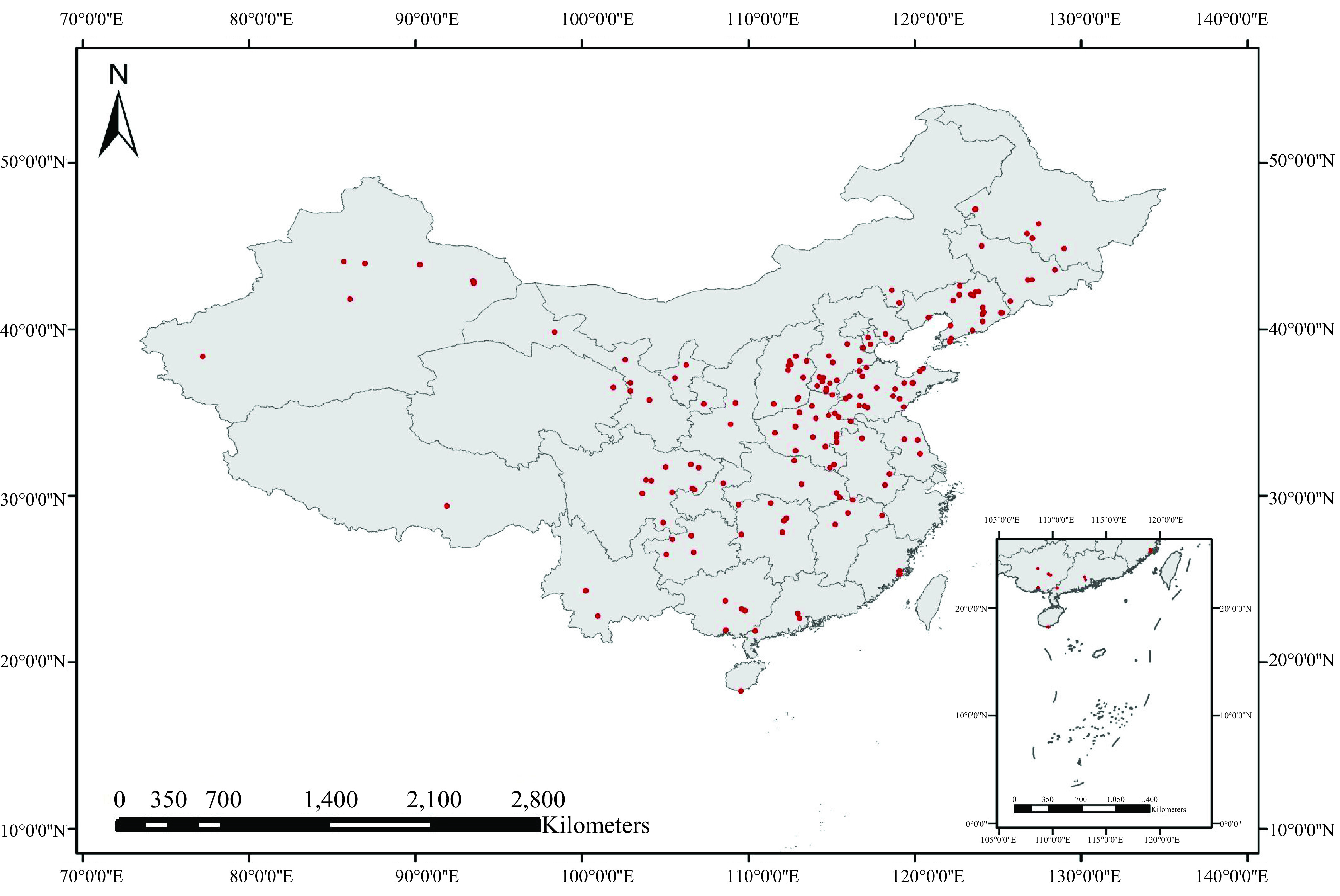
Locations and distribution of 166 groundwater sampling sites in the rural areas of China [Geographic coordinates of the sampling sites are listed in Excel Table S1. The map was created using ArcGIS 10.2 (ESRI)].

The present study did not consider temporal variation of the groundwater quality owing to the high stability of the groundwater relative to surface waters (Elçi and Polat 2011). Geographic coordinates of the sampling villages; sampling date and weather conditions; depth of the wells; and pH, temperature, and electrical conductivity of the groundwater samples are listed in Excel Table S1.

At each sampling well, $4\mathrm{L}$ groundwater was collected by student volunteers using pre-cleaned Teflon®-capped amber glass bottles. The samples for metal analysis were accommodated in $500\text{-mL}$ polypropylene bottles that had been soaked in nitric acid (20 wt%) for 24 h. The groundwater samples were collected by pumps, taps, or buckets. When pumps or taps were used, the wells were pumped for $5–10\text{\hspace{0.17em}min}$ beforehand to eliminate the influence of pipelines. When buckets were used, the buckets were rinsed three times with the groundwater before sampling. All the sampling vessels were prerinsed with the groundwater on site.

The groundwater samples were prevented from contacting plastic products (e.g., plastic buckets and plastic pots), transported to the laboratory within 48 h, and pretreated (pretreatment described in the section “Sample Pretreatment, Instrumental Analysis, and Statistical Analysis”) within 24 h upon arrival at the laboratory. During transportation, the samples were kept at low temperatures (4°C) with ice packs.

Sample Pretreatment, Instrumental Analysis, and Statistical Analysis

Analysis of SVOCs.

An automated identification and quantification system (AIQS) developed by Kadokami et al. (2005) was applied to analyze 886 SVOCs, including 17 alcohols, 54 substituted phenols, 13 PAEs, 50 esters, 6 amides, 78 PAHs, 26 $n$-alkanes, 20 substituted nitrobenzenes, 403 pesticides, 14 ethers, 15 chlorobenzenes, 16 substituted biphenyls, 34 substituted anilines, 63 polychlorinated biphenyls, 17 PPCP chemicals, 26 aliphatic acids, and 35 others. The AIQS has been successfully applied in previous studies (Li et al. 2016; Kong et al. 2015, 2016).

Phosphate buffer (monopotassium phosphate-potassium hydroxide, $1\text{\hspace{0.17em}mol}/\mathrm{L}$, pH 7.0) was added to a $500\text{-mL}$ water sample to adjust the pH to 7 (Li et al. 2016). The sample, spiked with $50\mathrm{\mu }\mathrm{L}$ surrogate standards (Excel Table S2; $10\mathrm{\mu }\mathrm{g}/\mathrm{mL}$ of each chemical), was passed through a glass membrane fiber (GMF) disk (Whatman® GMF 150, $47\mathrm{mm}$), a styrene-divinylbenzene (XD) disk (3M Empore™ styrenedivinylbenzene SDB-XD 2242, $47\mathrm{mm}$), and an active carbon (AC) disk (3M Empore™ activated carbon 2272, $47\mathrm{mm}$) under vacuum at a flow rate of $50\mathrm{mL}/\text{min}$.

After drying, the GMF and XD disks were eluted sequentially with $10\mathrm{mL}$ acetone and $5\mathrm{mL}$ dichloromethane, and the AC disk was eluted with $10\mathrm{mL}$ acetone. The eluates were combined and concentrated under a gentle stream of nitrogen (${\mathrm{N}}_2$) to $1\mathrm{mL}$. The concentrate was mixed with hexane to $10\mathrm{mL}$, dehydrated with anhydrous sodium sulfate, and concentrated to $0.5\mathrm{mL}$. Prior to instrumental analysis, $50\mathrm{\mu }\mathrm{L}$ internal standards [Excel Table S2; $10\mathrm{\mu }\mathrm{g}/\mathrm{mL}$, 8 isotope-labeled chemicals; Hayashi Pure Chemical (Kadokami et al. 2005)] were added. The target SVOCs were measured using an Agilent 6890-5975 gas chromatography–mass spectrometry (GC-MS) system operating in total ion monitoring mode and quantified using the AIQS (Kadokami et al. 2005). The GC-MS conditions are listed in Excel Table S3.

Analysis of POCs.

For POC analysis, the sample pretreatment method reported by the Kadokami group (Chau et al. 2017) was adopted. A liquid chromatography–quadrupole time-of-flight mass spectrometry (LC-QTOF/MS; Sciex X-500R) system was adopted to analyze 484 POCs, including 296 polar pesticides, 166 PPCP chemicals, 8 food additives, 10 industrial chemicals, and 4 others (Kadokami and Ueno 2019).

A groundwater sample ($500\mathrm{mL}$) was filtered through a glass fiber filter (Whatman® GF/C; $47\mathrm{mm}$) after adding $1\mathrm{mL}$ of phosphate buffer, ($1\text{\hspace{0.17em}mol}/\mathrm{L}$, pH 7.0) and $50\mathrm{\mu }\mathrm{L}$ surrogate standards ($4\mathrm{\mu }\mathrm{g}/\mathrm{mL}$ of each chemical; Excel Table S4). Subsequently, the filtrate was passed through an Oasis® HLB Plus cartridge (Waters) and a Sep-Pak® AC2 cartridge (GL Science) at a flow rate of $10\mathrm{mL}/\text{min}$. The cartridges were dried by passing a stream of ${\mathrm{N}}_2$ over them for $40\text{\hspace{0.17em}min}$, and then the analytes were eluted from the Sep-Pak® AC2 side with $5\mathrm{mL}$ methanol and $3\mathrm{mL}$ dichloromethane. Finally, $40\mathrm{\mu }\mathrm{L}$ internal standard [Excel Table S4; $5\mathrm{\mu }\mathrm{g}/\mathrm{mL}$ of each chemical; Kanto Chemical (Kadokami and Ueno 2019)] was added, and the mixture was reconstituted to $400\mathrm{\mu }\mathrm{L}$ with methanol. The solution was filtered with a syringe filter (Milliex® LG; Merck Millipore; $4\mathrm{mm}$) that had been preconditioned with $1\mathrm{mL}$ methanol.

The instrumental conditions of an LC-QTOF/MS–sequential window acquisition of all theoretical fragmention spectra acquisition adopted in the analysis are listed in Excel Table S5. The target POCs were identified using retention times, accurate masses of a precursor and two product ions, their ion ratios, and accurate MS/MS spectra (Kadokami and Ueno 2019). Quantitation of target POCs was performed by an internal standard method using precursor ions (Kadokami and Ueno 2019).

Analysis of metals.

The U.S. EPA Method 200.8 (U.S. EPA 1994) was adopted to determine 24 metals [lithium (Li), beryllium (Be), boron (B), titanium (Ti), vanadium (V), chromium (Cr), manganese (Mn), nickel (Ni), cobalt (Co), copper (Cu), zinc (Zn), gallium (Ga), arsenic (As), selenium (Se), rubidium (Rb), strontium (Sr), molybdenum (Mo), silver (Ag), cadmium (Cd), antimony (Sb), barium (Ba), thallium (Tl), lead (Pb), and thorium (Th)] with an inductively coupled plasma-mass spectrometry (ICP-MS; PerkinElmer NexION 300) system. A $10\text{-mL}$ sample (preserved with 32.5 wt% nitric acid, $\text{pH}<2$) was transferred into a $15\text{-mL}$ polypropylene centrifuge tube. If the nephelometric turbidity unit (NTU) of the sample was $<1,\text{\hspace{0.17em}then\hspace{0.17em}}0.2\mathrm{mL}$ nitric acid (32.5 wt%) was added to the $10\text{-mL}$ sample to adjust the acid concentration. If the $\text{NTU}>1,\text{\hspace{0.17em}then\hspace{0.17em}}0.2\mathrm{mL}$ nitric acid (32.5 wt%) and $0.1\mathrm{mL}$ hydrochloric acid solution (18.25 wt%) were added. The sample was then digested by heating in a water bath (85°C, 1.5 h). The 24 target metals were analyzed using an ICP-MS (PerkinElmer NexION 300), and the instrumental conditions are listed in Excel Table S6.

For mercury (Hg) analysis, a Chinese technical standard method (HJ 694-2014) (Ministry of Environmental Protection of China 2014) for sample pretreatment was followed. In short, $0.05\mathrm{mL}$ hydrochloric acid (36.5%) was added into $10\text{-mL}$ water samples for digestion. An atomic fluorescence spectrophotometer (AFS; HaiGuang AFS-9531) was employed to analyze Hg, and the AFS instrumental conditions are listed in Excel Table S7.

Quality control and assurance.

At least one laboratory blank was analyzed with each batch of 10 groundwater samples to check for potential sample contamination and interferences. Ultrapure water ($18\mathrm{M}\mathrm{\Omega }\times \mathrm{cm}$, OKP-series ultrapure water system; Lakecore Instrument Co.) employed as blank samples was prefiltered using the GMF, XD, and AC disks for the SVOC analysis, or by the HLB plus and Sep-Pak® AC2 cartridges for the POC analysis. The samples and blanks were analyzed simultaneously in the sampling periods. If analyte concentrations in the samples were two times higher than those in the blanks, the concentrations were reported by subtraction of the blank concentrations. Otherwise, the analyte was reported as not detected (n.d.).

For OMPs, the surrogate standards were spiked into 1/10 of the groundwater samples prior to extraction to check recovery and matrix effects. For metals, the recovery tests were conducted by spiking metal standards into $10\mathrm{mL}$ ultrapure water for ICP-MS analysis. Accuracy and precision for analysis of the metals were also assessed via replicate analysis of a standard reference material [National Metrology Institute in Japan certified reference material (NMIJ CRM) 7202-a No. 173 supplied by the National Institute of Advanced Industrial Science and Technology, Japan]. Recoveries of OMPs and metals were not employed to correct the concentrations of the detected species.

Calculation of carbon preference index.

To differentiate biogenic $n$-alkanes from those of petrogenic or anthropogenic origins, the carbon preference index (CPI) was calculated by the concentration ratio of odd-to-even–numbered $n$-alkanes (Mazurek and Simoneit 1984; Simoneit 1989). A $\text{CPI of}<1$ indicates important contributions from anthropogenic factors, a CPI close to 1 indicates that the alkanes mainly originated from petroleum, and a $\text{CPI of}<1$ indicates natural sources (Mazurek and Simoneit 1984).

Correlation between physicochemical properties of OMPs and their occurrence.

Physicochemical properties of the OMPs [e.g., water solubility (Sw) and $n$-octanol/water partition coefficient ($K_{\text{OW}}$)] were collected from the Estimation Program Interface (EPI) Suite (version 4.11; U.S. EPA 2012). Pearson correlation analysis was performed to examine the relationships between the properties and occurrence of the detected OMPs. Correlation was regarded as statistically significant if the significance level ($p$) was $\le 0.05$. All the statistical analyses were conducted using IBM SPSS Statistics (version 22).

Health Risk Assessment

Chronic daily intake.

The flowchart for the HRA is shown in Figure S1. Rural residents can be exposed to groundwater OMPs and metals through two primary pathways, drinking and showering. Risks caused by oral ingestion were generally one order of magnitude higher than by dermal absorption (Li et al. 2016). Hence, only oral ingestion was considered in the present study. Chronic daily intake ($\text{CDI}$; in milligrams per kilogram per day) was calculated as described by the U.S. EPA (1989):

$$\mathrm{C}\mathrm{D}\mathrm{I}=(\mathrm{C}\times \mathrm{I}\mathrm{R}\times \mathrm{E}\mathrm{F}\times \mathrm{E}\mathrm{D})/(\mathrm{B}\mathrm{W}\times \mathrm{A}\mathrm{T}\times {10}^3),$$ (1)

where C (in micrograms per liter) is the concentration of an assessed pollutant, IR (in liters per day) is the ingestion rate of drinking water, EF (in days per year) is the exposure frequency, ED (in years) is the exposure duration, BW (in kilograms) is the body weight, and AT (in days) is the average lifetime.

Noncarcinogenic risk assessment.

Noncarcinogenic risk, represented by the risk quotient for a specific pollutant $i$ (${\text{RQ}}_i$), was calculated by $\mathrm{R}{\mathrm{Q}}_i=\mathrm{C}\mathrm{D}{\mathrm{I}}_i/\mathrm{R}\mathrm{f}{\mathrm{D}}_i$ (U.S. EPA 1989), where $\mathrm{R}\mathrm{f}{\mathrm{D}}_i$ (in milligrams per kilogram per day) is the chronic $\text{RfD}$ for a specific pollutant. The cumulative noncarcinogenic risk for multiple pollutants was calculated as $\mathrm{R}{\mathrm{Q}}_{\mathrm{T}}=\sum _{i=1}^n\mathrm{R}{\mathrm{Q}}_i$, where $n$ stands for the number of assessed pollutants. The ${\text{RfD}}_i$ values were either retrieved from various databases/documents (Excel Table S8) or estimated by the CTV software (http://toxvalue.org; Wignall et al. 2018). For a given pollutant $i$, if the ${\text{RfD}}_i$ value was available from more than one database, the ${\text{RfD}}_i$ value was selected according to the hierarchy listed in Excel Table S8.

Because ${\text{RfD}}_i$ values for many pollutants are lacking, the values were also estimated based on the no observed adverse effect level (NOAEL; in milligrams per kilogram per day) or the lowest observed adverse effect level (LOAEL; in milligrams per kilogram per day):

$$Rf{D}_i=\left(NOAEL\text{\hspace{0.17em}or\hspace{0.17em}}LOAEL\right)/(U{F}_s\times MF),$$ (2)

where $MF$ (no units) is a modifying factor ranging from $>0$ to 10 and the default value is 1, and $U{F}_s$ (no units) is an uncertainty factor (U.S. EPA 1989). The NOAEL and LOAEL values were obtained from the various databases listed in Excel Table S8. $U{F}_s$ can be calculated as $U{F}_s=U{F}_1\times U{F}_2\times U{F}_3\times U{F}_4\times U{F}_5$, where $U{F}_1$ is uncertainty in extrapolating from a LOAEL rather than from a NOAEL, $U{F}_2$ is uncertainty in extrapolating from subchronic to chronic exposure, $U{F}_3$ is interspecies uncertainty, $U{F}_4$ is inter-individual variability, and $U{F}_5$ is uncertainty in extrapolation when the database is incomplete (U.S. EPA 1989). Considerations on the selection of $U{F}_s$ in relation to an available data set (U.S. EPA 2002) are described in Excel Table S9.

QSAR models in the CTV software (http://toxvalue.org; Wignall et al. 2018) were also adopted to predict the $\text{RfD}$ values (${\text{RfD}}_{\text{pre}}$) for pollutants with unavailable NOAEL and LOAEL data. The QSAR model for $\text{RfD}$ prediction had a mean error of units and its applicability domain covers $>80\%$ of environmental chemicals (Wignall et al. 2018). The $\text{RfD}$ values obtained from toxicity databases have a top priority of adoption, followed by those calculated by Equation (2). Only when no NOAEL and LOAEL data were available were the ${\text{RfD}}_{\text{pre}}$ values employed.

Carcinogenic risk assessment.

Carcinogenic risk (${\text{CR}}_i$) caused by a specific carcinogen for individuals developing cancer over a lifetime can be calculated as described by the U.S. EPA (1989):

$$\mathrm{C}{\mathrm{R}}_i=\mathrm{C}\mathrm{D}{\mathrm{I}}_i\times \mathrm{C}\mathrm{S}{\mathrm{F}}_{i,}$$ (3)

where $\mathrm{C}\mathrm{S}{\mathrm{F}}_i$ (in kilograms times day per milligram) is the carcinogenicity slope factor, which can be obtained from toxicity databases or predicted by QSARs. Herein carcinogens were identified from the detected pollutants according to the list of Group 1, 2A, 2B, and 3 carcinogens recommended by the International Agency for Research on Cancer (IARC 2020). The ${\text{CSF}}_i$ values of carcinogens were obtained from various toxicity databases (Excel Table S8) and a QSAR model in the CTV software (http://toxvalue.org; Wignall et al. 2018). The QSAR model for $\text{CSF}$ prediction has a mean prediction error of 0.92 ${\log }_{10}$ units (Wignall et al. 2018). Cumulative risk of carcinogens (${\text{CR}}_T$) was calculated by summing the ${\text{CR}}_i$ of each carcinogen.

Monte Carlo analysis.

To account for uncertainty in health risks caused by variation of the input parameter, a Monte Carlo analysis was performed based on statistical distributions of the input variables with 10,000 iterations. In the Exposure Factors Handbook of Chinese Population (Duan 2013), statistical parameters of ingestion rate (IR) were given with percentile values of 5%, 50%, and 95%, and statistical parameters of body weight (BW) were provided with means and standard deviations of normal distribution. Based on the available statistical parameters, the triangular distribution and normal distribution were chosen for IR and BW, respectively. Statistical distributions of exposure frequency (EF), exposure duration (ED), and average lifetime (AT) were adopted from the recommendations of the U.S. EPA (1996, 1989). Detailed statistical distributions of the input parameters are listed in Excel Table S10. The ${\text{RfD}}_i$ or ${\text{CSF}}_i$ values in the databases were considered as reliable, and their single-point values were adopted as the model inputs. The Monte Carlo simulation was performed with a script developed by Numpy (version 1.16.3) and Pandas (version 0.23.0) modules on Python (version 3.6.5).

Results

Quality Control and Assurance

Although precautions to avoid contamination were implemented, 45 organic compounds and 15 metals were still detected in the blanks (Excel Table S11). In the blanks of July 2016, 25 SVOCs were detected with their average concentrations of the individual analyte ($\overline{C}i$) in the range of $2.0\times {10}^{-3}$ $\text{to\hspace{0.17em}}0.53\mathrm{\mu }\mathrm{g}/\mathrm{L}$, 12 POCs were detected with $\overline{C}i$ ranging from $9{.4\times 10}^{-7}$ to $3.4\times {10}^{-3}\mathrm{\mu }\mathrm{g}/\mathrm{L}$, and 9 metals were detected with $\overline{C}i$ ranging from 0.018 to $0.3\mathrm{\mu }\mathrm{g}/\mathrm{L}$, except for Se ($7.8\mathrm{\mu }\mathrm{g}/\mathrm{L}$) and Zn ($3.7\mathrm{\mu }\mathrm{g}/\mathrm{L}$) (Excel Table S11). In the blank samples of February 2017, 19 SVOCs were detected with $\overline{C}i$ ranging from $2{.0\times 10}^{-3}$ to $0.24\mathrm{\mu }\mathrm{g}/\mathrm{L}$, 8 POCs were detected with $\overline{C}i$ ranging from $4.9\times {10}^{-5}$ to $0.037\mathrm{\mu }\mathrm{g}/\mathrm{L}$, and 10 metals were detected with $\overline{C}i$ ranging from 0.015 to $0.36\mathrm{\mu }\mathrm{g}/\mathrm{L}$, except for Mn ($9.2\mathrm{\mu }\mathrm{g}/\mathrm{L}$), Se ($2.2\mathrm{\mu }\mathrm{g}/\mathrm{L}$) and Zn ($1.3\mathrm{\mu }\mathrm{g}/\mathrm{L}$) (Excel Table S11). In the blank samples of July 2017, 15 SVOCs and 6 POCs were detected with $\overline{C}i$ of $7.8\times {10}^{-4}$–$0.21\mathrm{\mu }\mathrm{g}/\mathrm{L}$ and $6.6\times {10}^{-6}$– $0.16\mathrm{\mu }\mathrm{g}/\mathrm{L}$, respectively, and 5 metals were detected with $\overline{C}i$ ranging from 0.018 to $0.40\mathrm{\mu }\mathrm{g}/\mathrm{L}$, except for Mn ($3.8\mathrm{\mu }\mathrm{g}/\mathrm{L}$) and Se ($1.1\mathrm{\mu }\mathrm{g}/\mathrm{L}$) (Excel Table S11).

The average recoveries ($\overline{R}i$) for 12 surrogate standards ranged from 63.2% to 88.3% for GC-MS analysis, and for 5 surrogate standards, 65.8% to 104.9% for the LC-QTOF/MS analysis (Excel Table S12). $\overline{R}i$ for 24 metals ranged from 68.8% to 116.6%, except for Zn (157.0%) (Excel Table S13). By the analysis of a standard reference material (NMIJ CRM 7202-a No. 173), $\overline{R}i$ for 13 metals were found to range from 85.6% to 115.8% (Excel Table S13), indicating that the accuracy and precision for the analysis of metals were satisfactory.

Levels of Organic Micropollutants and Metals

Two hundred thirty-three OMPs, including 107 SVOCs and 126 POCs, were detected in at least one of the 166 samples (Excel Table S14), with the total concentration of all the detected OMPs in individual samples ($\mathrm{\Sigma }\text{OMPs}$) ranging from $2.9\text{\hspace{0.17em}ng}/\mathrm{L}$ to $1.7\times {10}^5\text{ng}/\mathrm{L}$ (Excel Table S15). As shown in Figure 2, 14 OMPs were detected in $\ge 30\%$ of the sampling sites (Excel Table S14), including cotinine with median to maximum concentrations of $0.56–48\text{\hspace{0.17em}ng}/\mathrm{L}$ among the different samples, sulfamethoxazole ($0.66–56\text{\hspace{0.17em}ng}/\mathrm{L}$), atrazine-desethyl (n.d.$–270\text{\hspace{0.17em}ng}/\mathrm{L}$), tetracosane (n.d.–$\mathrm{1,100}\text{\hspace{0.17em}ng}/\mathrm{L}$), carbendazim (n.d.–$77\text{\hspace{0.17em}ng}/\mathrm{L}$), nitrobenzene (n.d.–$130\text{\hspace{0.17em}ng}/\mathrm{L}$), azoxystrobin (n.d.–$4.2\text{\hspace{0.17em}ng}/\mathrm{L}$), fenuron (n.d.–$58\text{\hspace{0.17em}ng}/\mathrm{L}$), sucralose (n.d.–$\mathrm{4,200}\text{\hspace{0.17em}ng}/\mathrm{L}$), amantadine (n.d.–$\mathrm{1,900}\text{\hspace{0.17em}ng}/\mathrm{L}$), nonadecane (n.d.–$250\text{\hspace{0.17em}ng}/\mathrm{L}$), benzophenone-3 (n.d.–$360\text{\hspace{0.17em}ng}/\mathrm{L}$), diethyl phthalate (n.d.–$100\text{\hspace{0.17em}ng}/\mathrm{L}$), and 1,4-dichlorobenzene (n.d.–$44\text{\hspace{0.17em}ng}/\mathrm{L}$).

Figure 2.

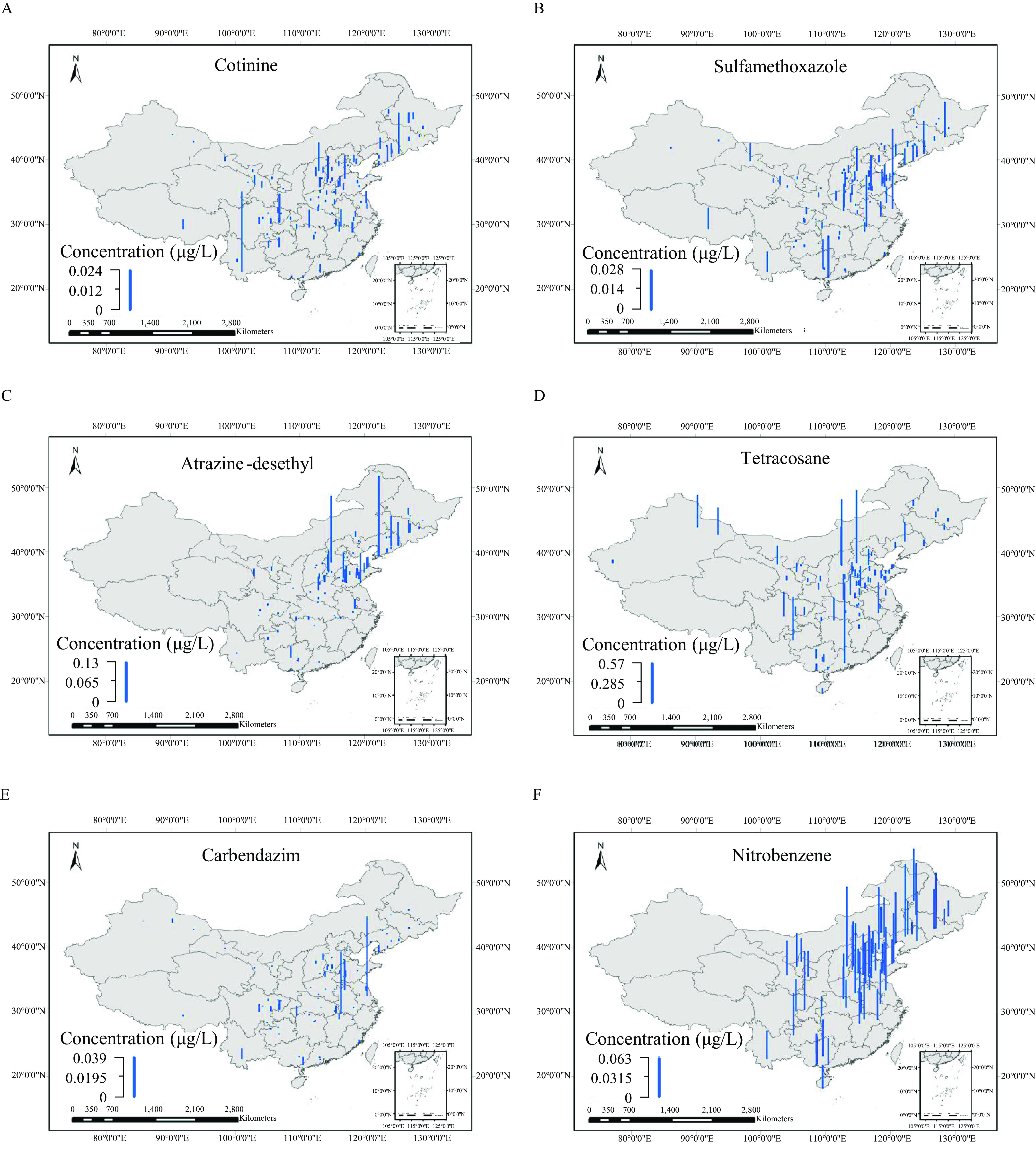
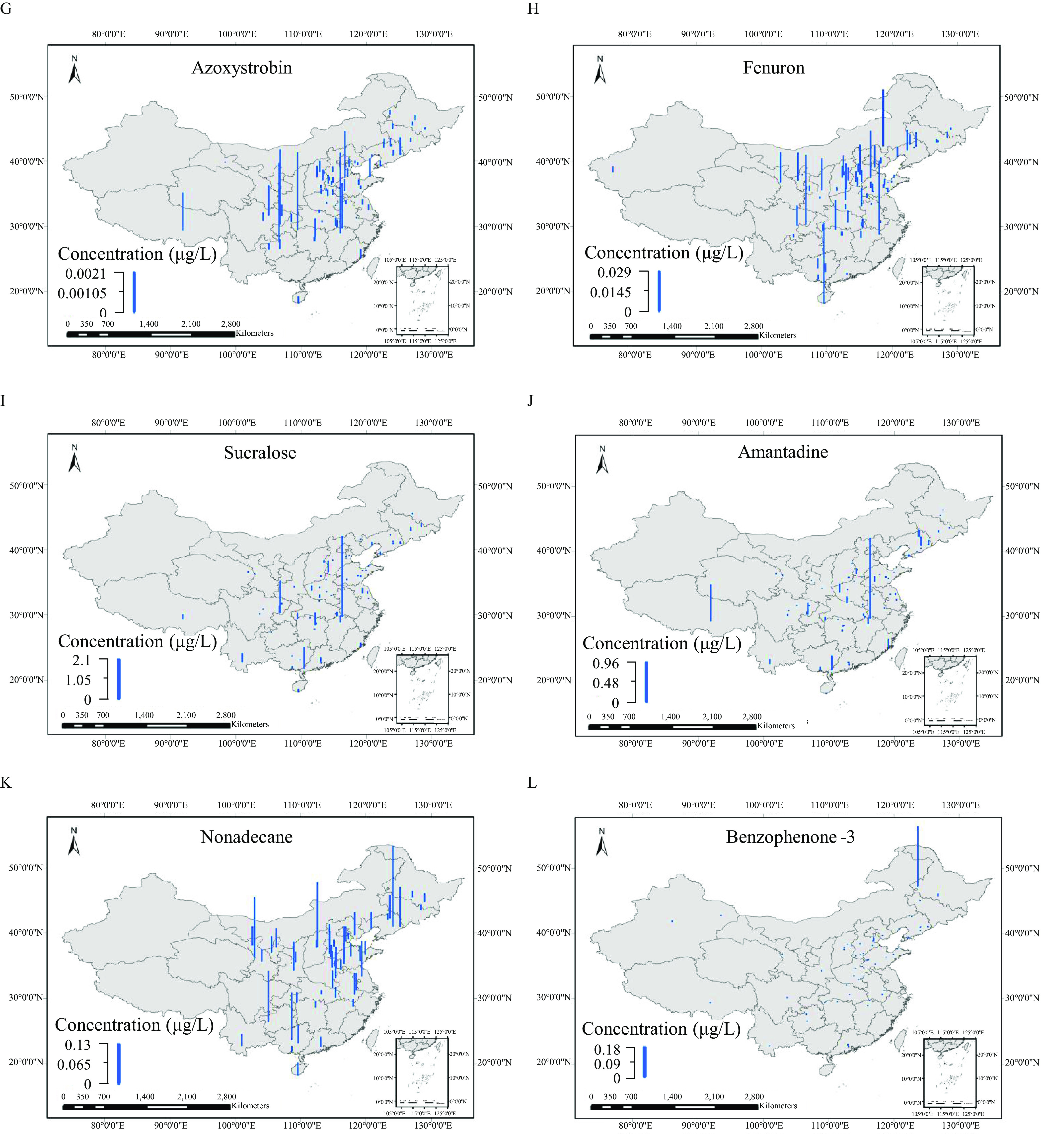
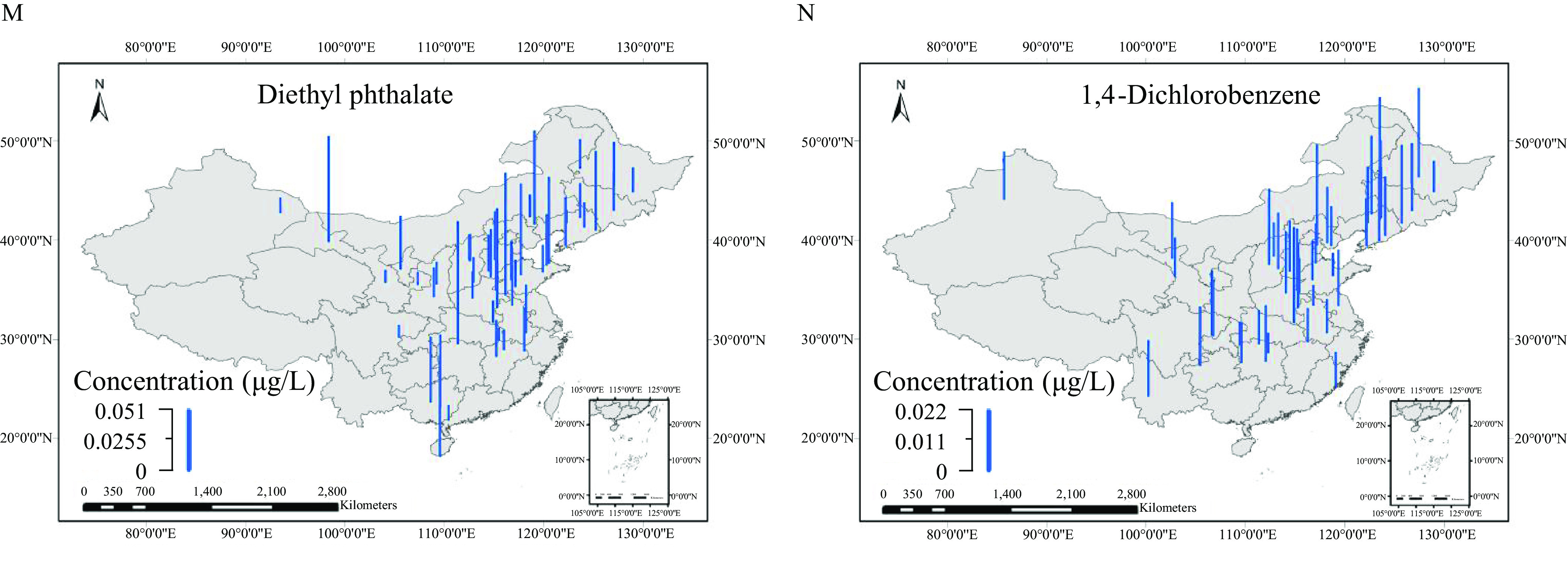
Spatial distribution for concentrations of (A) cotinine, (B) sulfamethoxazole, (C) atrazine-desethyl, (D) tetracosane, (E) carbendazim, (F) nitrobenzene, (G) azoxystrobin, (H) fenuron, (I) sucralose, (J) amantadine, (K) nonadecane, (L) benzophenone-3, (M) diethyl phthalate, and (N) 1,4-dichlorobenzene from the 166 samples. The blue bar heights represent the concentrations of each compound. [The corresponding data are listed in Excel Table S14. The map was created using ArcGIS 10.2 (ESRI)].

One hundred eighty-six of 233 detected OMPs exhibited the maximum concentrations of $<1\mathrm{\mu }\mathrm{g}/\mathrm{L}$. Despite this, in some areas of Liaoning, Shanxi, Hebei, Tianjin, and Guangxi, the samples contained high concentrations of the targets with $\mathrm{\Sigma }\text{OMPs}>50\mathrm{\mu }\mathrm{g}/\mathrm{L}$ (Excel Table S14). It was also found that detection frequencies of the OMPs detected in $>10\%$ of the 166 sites positively correlated with ${\log }_{10}{S}_{\mathrm{W}}$ for the OMPs [for OMPs with ${\log }_{10}{S}_{\mathrm{W}}$ (in micrograms per liter) $>1$, $n=28$, $r=0.31$, $p<0.05$, where $n$ stands for number of data points; Excel Table S16; Figure S2]. Similarly, as shown in Figure S3, POCs with detection frequencies $>1\%$ were more likely to be detected if they had low ${\log }_{10}{K}_{\text{OW}}$ values ($n=85$, $r=0.22$, $p<0.05$; Excel Table S17).

One hundred seven SVOCs were detected, including 17 substituted phenols, 10 PAEs, 13 PAHs, 22 $n$-alkanes, 3 nitrobenzenes, 9 pesticides, 7 alcohols, 3 dichlorobenzenes, 3 aliphatic acids, 4 esters, 2 amides, and 14 others (Excel Table S15). At least one SVOC was detected in 98% of the 166 sampling sites. According to the AIQS database, the detected SVOCs can be classified into domestic (business/household/traffic), industrial, and agricultural categories (Pan et al. 2014). Summed concentrations for the specific sources at each sampling site are listed in Excel Table S18. The calculated CPI values are listed in Excel Table S19, which shows that the values in 12.7% of the 166 sites were $\sim 1$, in 29.5% of the sites $<0.8$, in 28.9% of the sites $>1.2$, and 28.9% of 166 sites had no CPI values because no even-numbered n-alkane was detected. Of 484 POCs, 126 targets were detected in at least one of the 166 samples, including 52 PPCP chemicals (43 pharmaceuticals and 9 chemicals used in personal care products), 63 polar pesticides (19 insecticides, 22 herbicides, and 22 fungicides), 7 industrial chemicals, 2 food additives, and 2 others for which the concentrations are listed in Excel Table S15.

Twenty-five metals including 12 transition metals were detected in the groundwater samples (Excel Table S20). Sixteen metals were detected in $>50\%$ of the sampling sites. V (median–maximum: $1.3–57\mathrm{\mu }\mathrm{g}/\mathrm{L}$), B ($28–1.1\times {10}^4\mathrm{\mu }\mathrm{g}/\mathrm{L}$), Rb ($0.47–88\mathrm{\mu }\mathrm{g}/\mathrm{L}$), Li ($5.9–1.2\times {10}^3\mathrm{\mu }\mathrm{g}/\mathrm{L}$), Ni ($1.5–32\mathrm{\mu }\mathrm{g}/\mathrm{L}$), Ba ($56–1.8\times {10}^4\mathrm{\mu }\mathrm{g}/\mathrm{L}$), Ga ($8.5–89\mathrm{\mu }\mathrm{g}/\mathrm{L}$), and Sr ($7.4\times {10}^2–3.1\times {10}^5\mathrm{\mu }\mathrm{g}/\mathrm{L}$) exhibited detection frequencies of $>90\%$. Levels of Mn, Ba, Pb, Sb, B, Se, Ni, Cd, Hg, As, Tl, or Mo in at least one site were higher than the drinking-water standards of China (National Health Commission of China 2006), WHO (2017), or in some cases, of the United States (U.S. EPA 2018). Levels of Mn or Se in 18% of the sites exceeded the corresponding Grade III criterion of Chinese groundwater quality standard (GB/T 14848–2017) (Ministry of Land and Resources of China 2017).

Health Risk Assessment

${\mathrm{RfD}}_i$ and ${\mathrm{CSF}}_i$.

The $\text{RfD}$ values calculated with Equation (2) for 12 compounds (${\text{RfD}}_{\text{cal},i}$) were compared with those recorded in databases (Excel Table S21). The 12 compounds were selected because they had enough information that could be employed to calculate the ${\text{RfD}}_i$ values. As shown in Figure S4, there was good correlation between the calculated and recorded ${\text{RfD}}_i$ values with correlation coefficient $r=0.84$ ($n=12$, $p<0.05$), and mean error of 0.43 ${\log }_{10}$ unit, indicating that the ${\text{RfD}}_i$ calculation method was reliable. The mean error of ${\text{RfD}}_{\text{cal},i}$ values (0.43 ${\log }_{10}$ unit) was lower than the mean error (0.77 ${\log }_{10}$ unit) of the QSAR prediction that was reported by Wignall et al. (2018).

For 233 detected OMPs and 25 metals, the ${\text{RfD}}_i$ values retrieved from different databases (for 117 OMPs and 21 metals), calculated using the NOAEL or LOAEL (for 24 OMPs) (Excel Table S22) or estimated by the QSAR model (for 94 OMPs) are listed in Excel Table S23. However, the ${\text{RfD}}_i$ values for 5 substances, including octocrylene and 4 metals (Ga, Rb, Tl, and Th), could not be obtained. Hence, the noncarcinogenic risks caused by 232 detected OMPs and 21 metals were finally assessed. The ${\text{RfD}}_i$ values estimated by the QSAR model were considered less reliable for the compounds outside the applicability domain (Wignall et al. 2018). Sixty-five OMPs outside the applicability domain are noted in Excel Table S23.

Forty-four detected pollutants including 38 OMPs and 6 metals are in the WHO list of Group 1, 2A, 2B, and 3 carcinogens (IARC 2020). Their ${\text{CSF}}_i$ values retrieved from different databases (for 14 OMPs and 4 metals) or estimated by the QSAR model (for 24 OMPs) are listed in Excel Table S24. The ${\text{CSF}}_i$ values of Ni and Be could not be obtained. Therefore, the carcinogenic risks for 38 OMPs and 4 metals were assessed. The ${\text{CSF}}_i$ values estimated by the QSAR model were considered less reliable for the compounds outside the applicability domain (Wignall et al. 2018). Twenty-two OMPs outside the applicability domain are noted in Excel Table S24.

Noncarcinogenic risk.

After removing the 65 OMPs outside the model applicability domain, the ${\text{RQ}}_{\mathrm{T}}$ values for all the samples exhibited difference of $<10\%$ relative to those posed by 232 OMPs and 21 metals, except for five samples (Excel Table S25). For the five samples, the ${\text{RQ}}_{\mathrm{T}}$ were $<1$, even in the case of including the compounds outside the model applicability domain. Thus, the ${\text{RQ}}_{\mathrm{T}}$ values calculated by the 232 detected OMPs and 21 metals are discussed further.

The Monte Carlo simulations gave the fifth percentile, 50th percentile, 95th percentile, and average ${\text{RQ}}_i$ values (Excel Table S26). The average ${\text{RQ}}_{\mathrm{T}}$ for the detected OMPs and metals ranged from $1.9\times {10}^{-6}$ to 4 for most of the sampling sites, except for six sites in Ningxia (${\text{RQ}}_{\mathrm{T}}=12,29$), Yunnan (${\text{RQ}}_{\mathrm{T}}=12$), Heibei (${\text{RQ}}_{\mathrm{T}}=30$), Tianjin (${\text{RQ}}_{\mathrm{T}}=49$), and Shandong (${\text{RQ}}_{\mathrm{T}}=75$). Spatial distribution of ${\text{RQ}}_{\mathrm{T}}$ for OMPs and metals was estimated by inverse distance weighted interpolation (Goovaerts 2000) and is shown in Figure 3. The ${\text{RQ}}_{\mathrm{T}}$ values for 77% of the sampling sites were $<1$, indicating negligible risk to the residents. The other 23% sites had high risk with ${\text{RQ}}_{\mathrm{T}}>1$, indicating the groundwater was not suitable for drinking (Excel Table S25).

Figure 3.

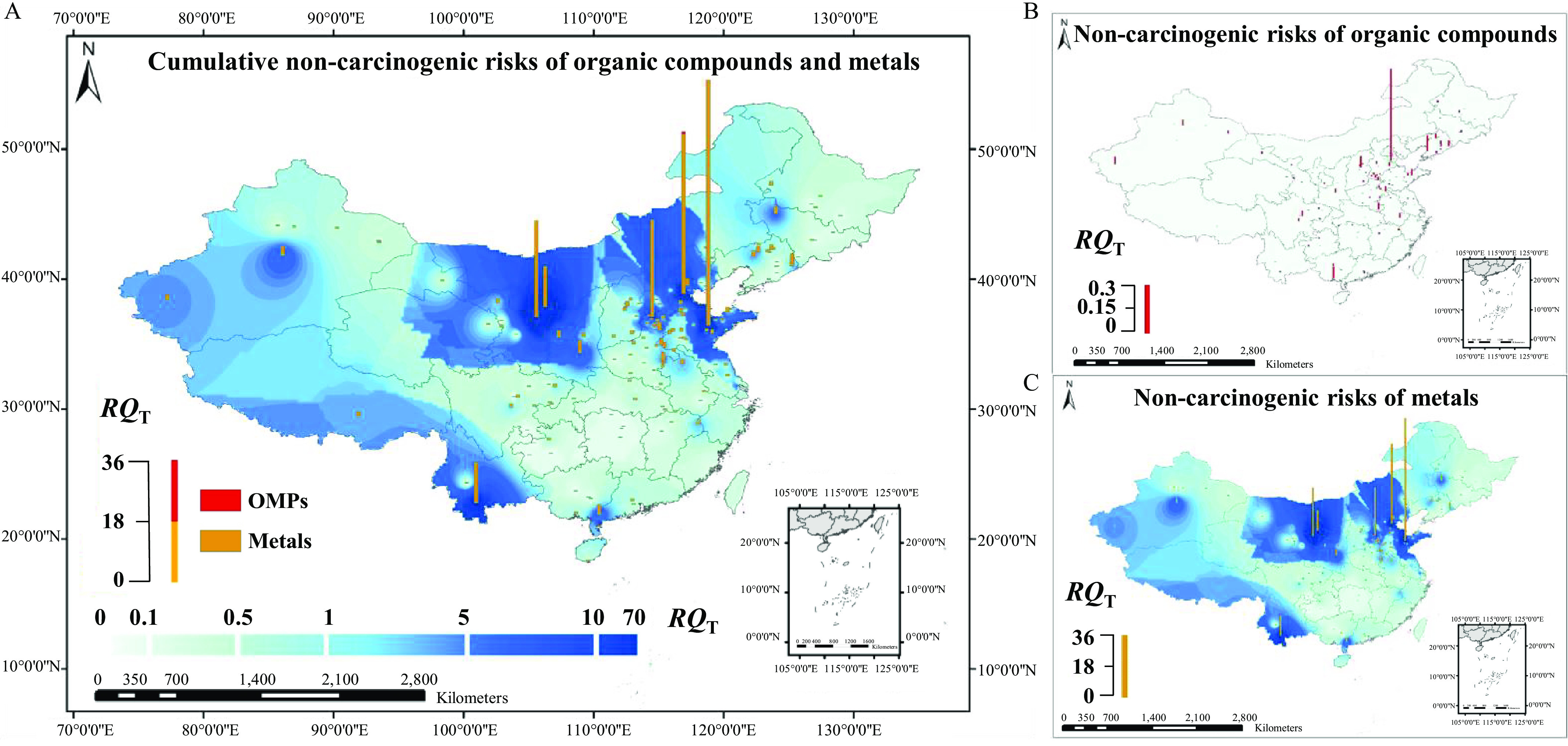
Spatial distribution of cumulative noncarcinogenic risks (${\text{RQ}}_{\mathrm{T}}$) for organic micropollutants (OMPs) and metals estimated by inverse distance weighted (IDW) interpolation. (The corresponding data are listed in Excel Table S25.) (A) Spatial distribution of ${\text{RQ}}_{\mathrm{T}}$ for 232 OMPs and 21 metals, (B) spatial distribution of ${\text{RQ}}_{\mathrm{T}}$ for 232 OMPs, and (C) spatial distribution of ${\text{RQ}}_{\mathrm{T}}$ for 21 metals. The red and yellow bar heights represent the ${\text{RQ}}_{\mathrm{T}}$ levels of OMPs and metals, respectively. $\mathrm{R}{\mathrm{Q}}_{\mathrm{T}}={\sum }_{i=1}^n\mathrm{R}{\mathrm{Q}}_i$, where $n$ stands for the number of assessed pollutants, and ${\text{RQ}}_{\mathrm{T}}$ is the risk quotient for a specific pollutant. The color gradient (light–dark blue) represents the ${\text{RQ}}_{\mathrm{T}}$ values estimated by IDW interpolation. [The map was created by using ArcGIS 10.2. (ESRI).]

The ${\text{RQ}}_{\mathrm{T}}$ values for the detected OMPs in all the sampling sites were $<1$ (Excel Table S25). However, the ${\text{RQ}}_{\mathrm{T}}$ values caused by the detected metals ranged from 0 to 75, contributing 96% (0–100%) of the total noncarcinogenic risks. High risks (${\text{RQ}}_{\mathrm{T}}>1$) of metals were observed in 22.6% of the sampling sites (Excel Table S25). Li, B, Co, As, Se, Sr, Mo, Cd, Sb, Ba, and Pb exhibited high ${\text{RQ}}_i$ values ($>1$) for at least one site. In particular, Li (${\text{RQ}}_i\le 21$), Sr ($\le 18$), Mo ($\le 17$), and Pb ($\le 55$) showed ${\text{RQ}}_i$ values of $>10$ for at least one site (Excel Table S25). Three metals (Li, As, and Sr) were identified with $>10\%$ contribution to the cumulative risks (Table 1).

Table 1.

95th Percentile and mean risks for the pollutants with over 10% contribution to cumulative risks (${\text{RQ}}_{\mathrm{T}}$ or ${\text{CR}}_{\mathrm{T}}$).

Substances	Health risks at the 166 sites				Contribution ratio [$\mathrm{\eta }$ (%)a (166 sites)]
	95th percentileb		Mean valueb
	Mean	Maximum	Mean	Maximum	Mean	Range
Noncarcinogenic risks (${\text{RQ}}_i$)
Li	0.56	38	0.3	20	24.4	0–91.3
As	0.47	12	0.25	6.4	19.9	0–84.4
Sr	0.63	32	0.34	17	16.4	0–91.5
Bis(2-ethylhexyl)phthalate	$4.6\times {10}^{-3}$	0.14	$2.5\times {10}^{-3}$	$7.6\times {10}^{-2}$	10.9	0–97.8
Carcinogenic risks (${\text{CR}}_i$)
As	$2.1\times {10}^{-4}$	$5.3\times {10}^{-3}$	$4.3\times {10}^{-5}$	$1.1\times {10}^{-3}$	49.2	0–99.8
Cr	$5.7\times {10}^{-5}$	$7.7\times {10}^{-4}$	$1.2\times {10}^{-5}$	$1.6\times {10}^{-4}$	25.5	0–99.8
Nitrobenzene	$2.7\times {10}^{-6}$	$1.6\times {10}^{-5}$	$1.6\times {10}^{-7}$	$6.5\times {10}^{-6}$	19.8	0–100
Bis(2-ethylhexyl)phthalate	$1.3\times {10}^{-6}$	$3.9\times {10}^{-5}$	$5.3\times {10}^{-7}$	$3.0\times {10}^{-5}$	18.1	0–100
Sulfamethoxazole	$1.2\times {10}^{-6}$	$2.0\times {10}^{-5}$	$2.4\times {10}^{-10}$	$3.8\times {10}^{-8}$	17.6	0–100

Note: As, arsenic; Cr, chromium; $\mathrm{C}{\mathrm{R}}_i$, carcinogenic risk for risk quotient for a specific pollutant $i$; $\mathrm{C}{\mathrm{R}}_{\mathrm{T}}$, cumulative carcinogenic risks; $\mathrm{R}{\mathrm{Q}}_i$, cumulative noncarcinogenic risk for a specific pollutant $i$; $\mathrm{R}{\mathrm{Q}}_{\mathrm{T}}$, cumulative noncarcinogenic risks; Li, lithium; Sr, strontium.

^a$\mathrm{\eta }$ was calculated as $\mathrm{\eta }=\mathrm{R}{\mathrm{Q}}_i/\mathrm{R}{\mathrm{Q}}_{\mathrm{T}}$ or $\mathrm{\eta }=\mathrm{C}{\mathrm{R}}_i/\mathrm{C}{\mathrm{R}}_{\mathrm{T}}$.

^b95% percentiles and mean values are from Monte Carlo simulations.

For the substances with $>10\%$ contribution to ${\text{RQ}}_{\mathrm{T}}$ (Table 1), the ${\text{RQ}}_i$ values in the present study were compared with those calculated using the U.S. EPA’s Regional Screening Levels (RSLs; U.S. EPA 2019b). The ${\text{RQ}}_i$ values from the RSLs were similar to those calculated using the $\text{RfDs}$ (Excel Table S27).

Carcinogenic risk.

After removing the 22 OMPs outside the model applicability domain, the ${\text{CR}}_{\mathrm{T}}$ values in 138 samples exhibited differences of $<10\%$ relative to those posed by 38 OMPs and 4 metals, whereas the ${\text{CR}}_{\mathrm{T}}$ values in the other 28 sites showed differences of 15.3–100% (Excel Table S28). The ${\text{CR}}_{\mathrm{T}}$ values generated by all the carcinogens are given in Figure 4 and Excel Table S28, and the ${\text{CR}}_{\mathrm{T}}$ values generated by the 16 OMPs and 4 metals are listed in Excel Table S28. To perform a relatively comprehensive risk assessment, the ${\text{CR}}_{\mathrm{T}}$ values calculated by the 38 OMPs and 4 metals are mainly discussed in the present study.

Figure 4.

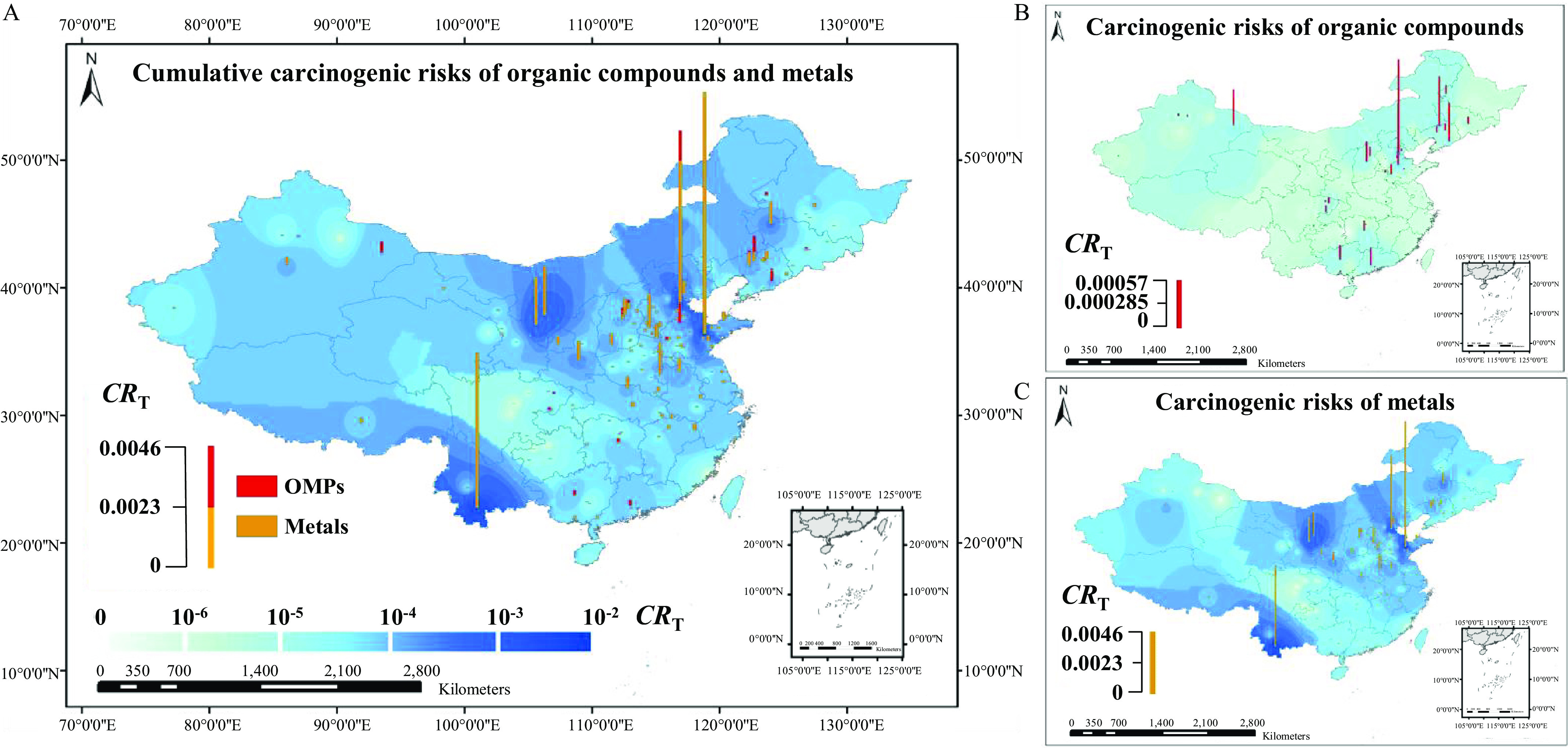
Spatial distribution of cumulative carcinogenic risks (${\text{CR}}_{\mathrm{T}}$) for organic micropollutants (OMPs) and metals estimated by inverse distance weighted (IDW) interpolation. (The corresponding data are listed in Excel Table S28.) (A) Spatial distribution of ${\text{CR}}_{\mathrm{T}}$ for 38 OMPs and four metals, (B) spatial distribution of ${\text{CR}}_{\mathrm{T}}$ for 38 OMPs, and (C) spatial distribution of ${\text{CR}}_{\mathrm{T}}$ for four metals. The red and yellow bar heights represent the ${\text{CR}}_{\mathrm{T}}$ values of OMPs and metals, respectively. $\mathrm{C}{\mathrm{R}}_{\mathrm{T}}={\sum }_{i=1}^n\mathrm{C}{\mathrm{R}}_i$, where $n$ stands for the number of assessed carcinogens, and ${\text{CR}}_i$ is the carcinogenic risk for a specific carcinogen $i$. The color gradient (light–dark blue) represents the ${\text{CR}}_{\mathrm{T}}$ levels estimated by IDW interpolation. (The map was created using ArcGIS 10.2 (ESRI).]

The Monte Carlo–simulated average cumulative carcinogenic risks (${\text{CR}}_{\mathrm{T}}$) for 42 carcinogens, including OMPs and metals, were up to $9.2\times {10}^{-3}$ (Figure 4; Excel Table S29). The ${\text{CR}}_{\mathrm{T}}$ values for 93% of the sample sites were $>{10}^{-6}$. For 34% of the sampling sites, the ${\text{CR}}_{\mathrm{T}}$ values were $>{10}^{-4}$ (Excel Table S28). The high ${\text{CR}}_{\mathrm{T}}$ values were caused mainly by the detected metals, which contributed 79% (0–100%) of the ${\text{CR}}_{\mathrm{T}}$ values. Two metals (As and Cr) were identified with $>10\%$ contribution to the cumulative risks (Table 1).

The OMP ${\text{CR}}_{\mathrm{T}}$ values for 48% of the 166 sites were $>{10}^{-6}$, and the values for 4.2% of the sites were $>{10}^{-4}$ (Excel Table S28). However, the metal ${\text{CR}}_{\mathrm{T}}$ values were $>{10}^{-6}$ for 87% of the 166 sites and $>{10}^{-4}$ for 28% of the sites (Excel Table S28). The metal ${\text{CR}}_{\mathrm{T}}$ value was up to $9.6\times {10}^{-3}$ at a site of Shandong (Figure 4; Excel Table S28). Three predominant OMPs (nitrobenzene, bis(2-ethylhexyl)phthalate, and sulfamethoxazole) were identified with a $>10\%$ contribution to the cumulative risks (Table 1).

For the substances with over 10% contribution to ${\text{CR}}_{\mathrm{T}}$ (Table 1), their ${\text{CR}}_i$ values were compared with those calculated using the RSL (U.S. EPA 2019b) method. The ${\text{CR}}_i$ values calculated by $\text{CSF}$ were about twice as high as those obtained from the RSL (Excel Table S27). This may be due to the fact that the exposure parameters used in the RSL method considers both adults and children (U.S. EPA 2019b), whereas only the exposure of adults were considered in the present study.

Discussion

Occurrence of OMPs in the Groundwater

To the best of the authors’ knowledge, this is the first comprehensive survey to reveal pollution of both OMPs and metals in the rural groundwater on a national scale in China and to assess health risks to the local residents. The present survey covered 28 provinces, municipalities, and autonomous regions and screened about 1,300 OMPs and 25 metals. Two hundred thirty-three OMPs and 25 metals were detected in at least one of the 166 groundwater samples/sites. The results may provide a benchmark data for future prioritization and risk assessment of OMPs and metals in the rural groundwater.

Excel Table S30 compares occurrences and concentrations of OMPs in the groundwater determined in the present study with those reported previously. The present study screened many more types of OMPs (more than 1,300 OMPs, including 886 SVOCs, 156 pharmaceuticals, 296 polar pesticides, 8 food additives, for example) than the previous studies, and detected more than 200 OMPs in the drinking groundwater samples. The previous large-scale surveys on OMPs in groundwater generally screened fewer target compounds (fewer than 300 compounds, including SVOCs, pharmaceuticals, and pesticides; Bexfield et al. 2019; Lapworth et al. 2015; Lopez et al. 2015).

PAEs, $n$-alkanes, pharmaceuticals, and pesticides were detected in the groundwater samples with $>70\%$ of detection frequency (Excel Table S15). The frequent occurrence of these pollutants can be related to their emission rates, degradation, migration, or background levels in the environment.

PAEs were found to be the dominant OMPs in the rural groundwater of China, contributing 26.5% (on average) of the $\mathrm{\Sigma }\text{OMPs}$ detected in each site (Excel Table S15). The high detection frequency and concentrations of PAEs may be attributed to their widespread use in plastic products (Balafas et al. 1999; Page and Lacroix 1995). PAEs are not chemically bound to the materials and, hence, can be easily released from plastic products into environments (Benjamin et al. 2015).

In particular, among all the detected PAEs, bis(2-ethylhexyl)phthalate (DEHP), dibutyl phthalate (DBP), and diethyl phthalate exhibited the highest contributions to the total concentrations of PAEs in the samples, and the mean contribution rates of DEHP, DBP, and diethyl phthalate were 28%, 12%, and 18%, respectively. As the most commonly used plasticizers, DEHP and DBP have been frequently detected in groundwater and surface waters, even in drinking-water samples of various countries and regions in the world (Zhang et al. 2009; YM Lee et al. 2019; Luo et al. 2018; Magdouli et al. 2013).

Stahlhut et al. (2007) demonstrated that concentrations of DEHP metabolites in human urine samples correlated significantly with abdominal obesity and insulin resistance. In the present study, DEHP concentrations in 10 of the 166 samples exceeded the drinking-water standard of $6\mathrm{\mu }\mathrm{g}/\mathrm{L}$ in the United States (U.S. EPA 2018), and in 8 of the 166 samples, exceeded the WHO drinking-water standard of $8\mathrm{\mu }\mathrm{g}/\mathrm{L}$ (WHO 2017). DBP concentration limits in drinking water are not regulated by the drinking-water standards in China (National Health Commission of China 2006), the United States (U.S. EPA 2018), and the WHO (2017). Although only 5% of the 166 samples exhibited DEHP levels exceeding the water quality standards, the health effects of PAEs still need to be evaluated in the future because only a few phthalates were considered in the drinking-water quality standards.

Twenty-two $n$-alkanes were detected in the groundwater with a detection frequency of 79.5% (Excel Table S15). The high detection frequency of $n$-alkanes could be caused by their wide range of sources, such as anthropogenic sources including coal combustion and petroleum products and natural sources including higher plant wax, bacteria, and alga (Simoneit 1984, 1986; Cheng et al. 2016). In previous studies, the CPI values have been used to differentiate biogenic $n$-alkanes from those of petrogenic or anthropogenic origins (Górka et al. 2014; Mille et al. 2007). In the present study, the CPI values in 12.7% of the 166 samples were approximately 1 and were distributed across Xinjiang, Ningxia, Gansu, Shanxi, Henan, Hebei, Hunan, Hubei, Shandong, Liaoning, and Anhui (Excel Table S19), suggesting that the alkanes in these sites mainly originated from petroleum. In fact, most of the sampling sites with CPI of approximately 1 were adjacent to oil fields (China Geological Survey 2015). The CPI values in 29.5% of the sampling sites were $<1$ (Excel Table S19), indicating contributions to $n$-alkanes from anthropogenic factors. Nevertheless, there is no evidence that $n$-alkanes in drinking water can cause adverse health effects, as far as the authors know.

Forty-three pharmaceuticals were detected in the groundwater, including 18 antibiotics, 8 cardiovascular system drugs, 3 hormones, 6 anti-inflammatories, 2 anti-allergic agents, and 2 psychotherapeutic drugs. At least one pharmaceutical was detected in 132 of the 166 groundwater samples. Antibiotics were dominant pharmaceuticals in the groundwater samples and contributed 65.8% (0–100%, average: 65.8%) to the total concentration of pharmaceuticals. Zhang et al. (2015) estimated that 162,000 tons of antibiotics were used in 2013 in China. Abuse of antibiotics led to the residues of antibiotics, not only in the groundwater of China, but also in the groundwater of various countries and regions of the world (Dong et al. 2018; HJ Lee et al. 2019; Mirzaei et al. 2018). The total concentrations of antibiotics in the present study (n.d.–$2.0\mathrm{\mu }\mathrm{g}/\mathrm{L}$) were higher than those detected from a study in Korea (n.d.–$0.0493\mathrm{\mu }\mathrm{g}/\mathrm{L}$; HJ Lee et al. 2019).

Sulfamethoxazole was a dominant antibiotic and contributed 49.2% (0–100%, average: 49.2%) of the total antibiotics. The high detection frequency and levels of sulfamethoxazole may be attributed to its widespread use. In China, the total usage of sulfamethoxazole in 2013 was estimated to be 313 tons (Zhang et al. 2015). Meanwhile, sulfamethoxazole is difficult to biodegrade ($t_{1/2}>100\mathrm{d}$; Benotti and Brownawell 2009), which may also partly explain its frequent occurrence. It is worth mentioning that sulfamethoxazole can cause antimicrobial resistance (Brosh-Nissimov et al. 2019), and groundwater is considered an important environment where antimicrobial resistance can spread (Andrade et al. 2020).

To the best of the authors’ knowledge, amantadine as an antiviral drug was detected in the groundwater of China for the first time in the present study. In China, the use of amantadine in livestock and poultry farming has been banned (Ministry of Agriculture of China 2005). The high detection frequency (39.2%) and level (up to $\mathrm{1,900}\text{\hspace{0.17em}ng}/\mathrm{L}$) of amantadine in the groundwater suggest an alternative source for this compound, such as illegal veterinary use. Another reason for the high detection frequency and level can be high environmental persistence of the compound, although environmental degradation data for the compound are not available. The EPI Suite (version 4.11; U.S. EPA 2012) has estimated that the time required for ultimate biodegradation of amantadine is several weeks to months.

In 7.2% of the groundwater samples, the sum concentrations of 72 pesticides exceeded the sum limit for pesticides ($500\text{\hspace{0.17em}ng}/\mathrm{L}$), an EU groundwater standard for pesticides (EC 2006). Levels of 15 individual pesticides exceeded the EU limit value of $100\text{\hspace{0.17em}ng}/\mathrm{L}$, including diuron (17/166), cinmethylin (6/166), tridemorph (3/166), fomesafen (2/166), imidacloprid (2/166), metolachlor (2/166), atrazine-desethyl (2/166), acetochlor (1/166), acetamiprid (1/166), aldicarb sulfoxide (1/166), chlorantraniliprole (1/166), clothianidin (1/166), prometryne (1/166), chlorimuron-ethyl (1/166), and penoxsulam (1/166). In addition, 3 pesticides that have been banned in China were detected at low detection frequency and concentrations, including chlorsulfuron (1.2%, n.d.–$20\text{\hspace{0.17em}ng}/\mathrm{L}$), metsulfuron-methyl (3.6%, n.d.–$57\text{\hspace{0.17em}ng}/\mathrm{L}$), and ethametsulfuron-methyl (1.2%, n.d.–$76\text{\hspace{0.17em}ng}/\mathrm{L}$). It has been shown that chlorsulfuron has developmental toxicity on rats (NCBI 2005a) and that metsulfuron-methyl has reproductive toxicity on rabbits (NCBI 2005b). However, to the best of the authors’ knowledge, there were no data available on the health effects of these pesticides to humans.

Occurrence of Metals in the Groundwater

Compared with previous large-scale surveys that focused only on toxic metals (i.e., As and Cr) in groundwater (Excel Table S31), the present study screened more types of metals in the groundwater samples from the rural areas in China. Six detected metals, Cr, Pb, Cd, Be, Ni, and As are in the IARC list of Group 1, 2A, 2B, and 3 carcinogens (IARC 2020). Among the six carcinogens, Ni, As, Cr, and Pb were frequently detected in the current groundwater samples, with detection frequencies of 92.7%, 86.0%, 70.1%, 37.8%, respectively.

Cr was detected with a median concentration of $0.77\mathrm{\mu }\mathrm{g}/\mathrm{L}$ (n.d.–$25\mathrm{\mu }\mathrm{g}/\mathrm{L}$), and a similar level was reported in Melen, Belgium ($1.5\mathrm{\mu }\mathrm{g}/\mathrm{L}$; Sengorur et al. 2015). The Pb concentrations (n.d.–$2.2\times {10}^3\mathrm{\mu }\mathrm{g}/\mathrm{L}$) in the groundwater samples were higher than those in South Africa ($2–26\mathrm{\mu }\mathrm{g}/\mathrm{L}$; Edokpayi et al. 2018) and India ($47–552\mathrm{\mu }\mathrm{g}/\mathrm{L}$; Chabukdhara et al. 2017). The As concentrations in the present study (n.d.–$56\mathrm{\mu }\mathrm{g}/\mathrm{L}$) were similar to those in the Melen watershed, Turkey (n.d.–$44\mathrm{\mu }\mathrm{g}/\mathrm{L}$; Sengorur et al. 2015); lower than the concentrations reported in Yin Chuan, China ($<1–177\mathrm{\mu }\mathrm{g}/\mathrm{L}$; Han et al. 2013), Datong basin, China ($<1–947.6\mathrm{\mu }\mathrm{g}/\mathrm{L}$; Zhang et al. 2017), Bangladesh ($2.76–462\mathrm{\mu }\mathrm{g}/\mathrm{L}$; Selim Reza et al. 2010); and higher than those in Huaibei Plain, China (n.d.–$27.2\pm 1.36\mathrm{\mu }\mathrm{g}/\mathrm{L}$; Hu et al. 2015). The Ni concentrations in the present study (n.d.–$32\mathrm{\mu }\mathrm{g}/\mathrm{L}$) were higher than those reported in Bay County, Xinjiang ($0.9–1.2\mathrm{\mu }\mathrm{g}/\mathrm{L}$; Turdi and Yang 2016) but lower than those reported in Uttar Pradesh, India (n.d.–$168\mathrm{\mu }\mathrm{g}/\mathrm{L}$; Chabukdhara et al. 2017) and Melen Watershed, Turkey (n.d.–$509\mathrm{\mu }\mathrm{g}/\mathrm{L}$; Çelebi et al. 2015).

Correlative Factors and Tracers on the Occurrence of the OMPs

The relationships between the physicochemical properties and the occurrence of the pollutants (Figures S2 and S3; Excel Tables S16 and S17) suggest that POCs with low hydrophobicity tend to migrate into groundwater favorably. Bexfield et al. (2019) also reported that compounds with high ${\log }_{10}{S}_{\mathrm{W}}$ or low ${\log }_{10}{K}_{\text{OW}}$ values tended to be present in groundwater.

In the present study, sucralose (n.d.–$\mathrm{4,200}\text{\hspace{0.17em}ng}/\mathrm{L}$), an artificial sweetener, was detected in the groundwater with a detection frequency of 40%. Sucralose has been frequently detected in the groundwater of many regions worldwide, including Canada (n.d.–$24\mathrm{\mu }\mathrm{g}/\mathrm{L}$; Van Stempvoort et al. 2011), the Ganges River Basin, India ($0.0005–0.025\mathrm{\mu }\mathrm{g}/\mathrm{L}$; Sharma et al. 2019), and the Dongjiang River Basin, China ($0.0468–2.44\mathrm{\mu }\mathrm{g}/\mathrm{L}$; Yang et al. 2018). The levels of sucralose was found to correlate with that of pharmaceuticals ($n=166$, $r=0.79$, $p<0.001$). The pharmaceuticals were wastewater-related pollutants and have been frequently detected in sewage treatment plants (McCance et al. 2018; Tran et al. 2014). Previous studies employed artificial sweeteners, such as acesulfame (Tran et al. 2014; Van Stempvoort et al. 2011) and saccharin (Buerge et al. 2011), as molecular tracers of sewage pollution in aquatic environments due to their recalcitrance to transformation and their low adsorption capacities on soils (Khazaei and Milne-Home 2017; Robertson et al. 2016a; Tran et al. 2014). Robertson et al. (2016b) indicated that degradation of sucralose occurs slowly in groundwater over a period of several months to several years. Therefore, sucralose may also be used as a pollution tracer for pharmaceuticals in groundwater.

The concentrations of sulfamethoxazole also correlated with those of other pharmaceuticals ($n=166$, $r=0.41$, $p<0.001$). Sulfamethoxazole has also been considered as a wastewater tracer in groundwater (McCance et al. 2018; Van Stempvoort et al. 2013). The concentrations of cotinine, a metabolite of nicotine, correlated with the levels of POCs ($n=166$, $r=0.36$, $p<0.001$). Cotinine has been commonly detected in wastewater (Karpuzcu et al. 2014; Buszka et al. 2009; Ferguson et al. 2013), and cotinine in groundwater has been attributed to urban sewage sources in previous studies (Karpuzcu et al. 2014).

Strategy for Comprehensive Risk Assessment

Due to the lack of ${\text{RfD}}_i$ and ${\text{CSF}}_i$ values, an HRA was conducted for a limited number of detected pollutants in many previous studies. In the present study, if the ${\text{RfD}}_i$ values were not available from databases, they were extrapolated from existing toxicity data or predicted using the QSARs. Monte Carlo simulation was performed to account for uncertainties in the exposure parameters and toxicity thresholds (${\text{RfD}}_i$ and ${\text{CSF}}_i$). Uncertainties of the toxicity thresholds from different sources were assessed by assuming specific triangular distribution for the ${\text{RfD}}_i$ and ${\text{CSF}}_i$ values. QSARs, together with the Monte Carlo simulation, may provide a feasible way to assess health risks of the large and ever-increasing number of pollutants detected in the environment.

Health Risks of OMPs

In the U.S. EPA Superfund program, a screening criterion set to one in one million (i.e., excess acceptable lifetime cancer risk greater than one in a million) was used as a threshold for the ${\text{CR}}_{\mathrm{T}}$ (U.S. EPA 2000), in which areas with ${\text{CR}}_{\mathrm{T}}>{10}^{-4}$ were considered to be unacceptable and to require remediation, with ${10}^{-6}<{\text{CR}}_{\mathrm{T}}<{10}^{-4}$ needed to be considered for remediation, and ${\text{CR}}_{\mathrm{T}}<{10}^{-6}$ were acceptable. Although over 200 OMPs were detected in the groundwater, the cumulative noncarcinogenic risks of the OMPs were acceptable to the local rural residents. However, the ${\text{CR}}_{\mathrm{T}}$ values for the OMPs in 48% of the sites were $>{10}^{-6}$, implying that the carcinogenic risks caused by the OMPs cannot be ignored (Figure 4). Three OMPs were significant contributors to the ${\text{CR}}_{\mathrm{T}}$ values: nitrobenzene [contribution rate: $\text{mean}\pm \text{standard\hspace{0.17em}deviation\hspace{0.17em}}\left(\text{SD}\right)$, $19.8\%\pm 30.1\%$], DEHP ($18.1\%\pm 33.1\%$), and sulfamethoxazole ($17.6\%\pm 31.3\%$).

Nitrobenzene is widely used in the production of pesticides, dyes, pharmaceuticals, and textiles (U.S. EPA 2019a) and is a main pollutant in the global aquatic environment (J Gao et al. 2008; S Gao et al. 2012). Nitrobenzene was observed in 42% of the sites, and its ${\text{CR}}_i$ values in four sites were $>{10}^{-6}$. It has been proved that exposure to nitrobenzene may lead to increase in incidence of mammary gland neoplasms, hepatocellular and renal neoplasms, and endometrial stromal neoplasms in mice and rats (Cattley et al. 1994).

DEHP was also a dominant pollutant in the groundwater. The ${\text{CR}}_i$ values of DEHP in 11% of the sites was $>{10}^{-6}$. Some previous studies also indicated DEHP to be a dominant pollutant in groundwater worldwide (Gani et al. 2017; Liu et al. 2014; Torres et al. 2018), with significant contributions to health risks to residents who consume groundwater for drinking (Geng et al. 2016).

Sulfamethoxazole was detected in 56% of the sites, and the ${\text{CR}}_i$ value was $>{10}^{-6}$ in one site of Jiangsu and one site of Jiangxi. However, the ${\text{CSF}}_i$ of sulfamethoxazole predicted by the CTV software may be unreliable given that the compound lies outside the applicability domain of the QSAR model, something which needs further investigation. Moreover, 4-aminobiphenyl, a Group 1 carcinogen in the IARC list (IARC 2020), was detected in six sites, and the corresponding ${\text{CR}}_i$ values were $>{10}^{-6}$. Even at one site in Guangxi, the corresponding ${\text{CR}}_i$ value was $>{10}^{-4}$. 4-aminobiphenyl, an intermediate of dyes and used as a rubber antioxidant (NCBI 2004), has been detected in cigarette smoke and hair dyes (Turesky et al. 2003; Bie et al. 2017).

Health Risks of Metals

The top three metals with large ${\text{RQ}}_i$ values were Li (contribution ratio, $\text{mean}\pm \text{SD}$: $24.4\%\pm 18.2\%$), As ($19.9\%\pm 19.4\%$), and Sr ($16.4\%\pm 16.5\%$). Two metals, As ($49.2\%\pm 37.6\%$) and Cr ($25.5\%\pm 32.3\%$), were significant contributors to the ${\text{CR}}_{\mathrm{T}}$ values. Among the three metals with high contributions to ${\text{RQ}}_{\mathrm{T}}$, Li and Sr were indispensable trace elements to humans (Liu et al. 2018; Schrauzer 2002) and have been widely detected in groundwater worldwide (Duggal et al. 2017; Edet et al. 2004; Giri and Singh 2015; Golubkina et al. 2018; Iqbal and Shah 2012; Kavanagh et al. 2017; Kent and Landon 2016; Purushotham et al. 2017; Qi et al. 2019; Toccalino et al. 2012; Voutchkova et al. 2018). Previous studies have indicated that the levels of Li or Sr in groundwater were not associated with noncarcinogenic risks (Duggal et al. 2017; Edet et al. 2004; Giri and Singh 2015; H Zhang et al. 2018). In the present study, however, the noncarcinogenic risks caused by Li or Sr were high (${\text{RQ}}_i>1$) in 3.0% and 3.6% of the 166 sites, respectively. The high ${\text{RQ}}_i$ values of Li were found at 2 sites in Xinjiang, 2 sites in Ningxia, and 1 site in Shanxi (Excel Table S25). For Sr, the high ${\text{RQ}}_i$ values were found at 2 sites in Ningxia, 1 site in Xinjiang, 1 site in Tianjin, 1 site in Hebei, and 1 site in Shandong (Excel Table S25).

Arsenic was detected in 86% of the sites, with a high contribution to the noncarcinogenic and carcinogenic risks. High As risks were identified in the sites in Tianjin, Hebei, Liaoning, Jilin, Xinjiang, Inner Mongolia, He’nan, Shandong, and Jiangsu provinces. Many previous studies focused on health risks of As in groundwater (Ahmed et al. 2019; Buschmann et al. 2008; Camacho et al. 2011; Kumar et al. 2016; Rodríguez-Lado et al. 2013). Rodríguez-Lado et al. (2013) also pointed out that high As risks are associated with areas in Xinjiang, Inner Mongolia, He’nan, Shandong, and Jiangsu provinces.

The ${\text{CR}}_i$ values of Cr in 68% of the sites exceeded ${10}^{-6}$ and, in 6% of the sites, exceeded ${10}^{-4}$. Nevertheless, the carcinogenic risk may be overestimated given that Cr concentrations measured using ICP-MS were assumed to be contributed completely by ${\mathrm{Cr}}^{\text{VI}}$. Further studies are needed to differentiate different Cr species in the groundwater.

The carcinogenic risk results (Figure 4) could be partly corroborated by the cancer morbidity and distribution in China. Gong and Zhang (2013) indicated that Tianjin, He’nan, Hebei, Shandong, Shanxi, Anhui, and Yunnan have more cancer villages or higher cancer village densities than the other provinces, and those provinces were also identified with high carcinogenic risks in the present study. The term cancer village refers to a geographic area for which cancer morbidity or mortality is remarkably higher than the national averages (Gong and Zhang 2013). According to data from the National Cancer Central Registry of China, cancer incidences decrease from the eastern to the central and western regions of China (Sun et al. 2019). In the present study, the carcinogenic risks for the sites in the eastern, central, and western areas [based on the national administrative division system of China (Sun et al. 2019)] were $0–6.0\times {10}^{-3}$ (median: $8.6\times {10}^{-5}$), $6.4\times {10}^{-6}\text{\hspace{0.17em}to\hspace{0.17em}}9.6\times {10}^{-3}$ (median: $7.5\times {10}^{-5}$), and $0–6.1\times {10}^{-3}$ (median: $4.2\times {10}^{-5}$), respectively. Therefore, the carcinogenic risk assessment results in the present study coincide with the general cancer incidence registry data in China.

Given that the Monte Carlo simulation adopted in the HRA in the present study took into consideration the distributions of the input parameters, the present study was able to provide a more reasonable estimation on the health risks for the adults using the groundwater for drinking than a conventional HRA based on a single value of input parameters. Nevertheless, the present study still has limitations.

• Although 166 drinking-water wells in the 166 villages from the 28 provinces, municipalities, and autonomous regions across China were sampled, the number of the samples is still too limited to accurately reflect the pollution status of rural groundwater use in China. In addition, field blanks were not collected due to the difficulty in sampling and transportation. For several provinces, the small number of the sampling sites or even the lack of samples, may also have led to high uncertainties in the estimation of the health risks. The regions with no samples (Beijing, Shanghai, Zhejiang, Hongkong, Macao, Taiwan) are more developed and, therefore, the groundwater for which may be polluted more seriously than for the other provinces. Nevertheless, this sampling defect may not necessarily influence the health risk estimates for the mainland of China given that few people employ groundwater directly for drinking in Beijing, Shanghai, and Zhejiang.

• OMPs degradation or elimination in processes such as boiling or cooking were not considered. These processes are common practice for Chinese. The overlook of these processes definitely leads to overestimation of OMP daily exposure.

• In the screening-level assessment of the cumulative risks, potential interactions and joint toxicity effects of the detected pollutants (e.g., synergy and antagonism) were not considered, which may have led to uncertainties in the cumulative risks. Only oral ingestion was considered in the risk calculations, which may underestimate the risks.

• Point values of ${\text{RfD}}_i$ were employed in the HRA of the present study. Nevertheless, as pointed out by Chiu et al. (2018), the toxicity values themselves are not actually point values. Chiu et al. (2018) provided a probabilistic approach to derive ${\text{RfD}}_i$ values. The application of point values of ${\text{RfD}}_i$ may also lead to unknown uncertainties in the HRA.

• To comprehensively estimate the health risks, the ${\text{RfD}}_i$ values for 65 OMPs and the ${\text{CSF}}_i$ values for 22 OMPs predicted using the QSARs (http://toxvalue.org; Wignall et al. 2018) were adopted. Nevertheless, these compounds lie outside the applicability domains of the respective QSAR models, which may also lead to unknown uncertainties in the HRA. The situation also indicates that further efforts to develop QSAR models with large applicability domains are necessary.

To the best of our knowledge, albeit with the above limitations, the significance of the present study as the first and most comprehensive survey of OMPs and metals in the rural groundwater in China, as well as the first comprehensive HRAs of groundwater for drinking, cannot be diminished.

In summary, a panoramic and elementary view of OMPs and metals pollution in the rural groundwater of China and the related health risk estimates were unveiled and may provide a benchmark for future efforts to monitor rural groundwater quality and for ensuring the safety of drinking water for rural residents in China. The joint application of the QSARs and the Monte Carlo simulation may provide a feasible way to assess health risks of the large and ever-increasing number of pollutants detected in the environment.

References

- Abey JA, Adebiyi FM, Asubiojo OI, Tchokossa P. 2017. Assessment of radioactivity and polycyclic aromatic hydrocarbon levels in ground waters within the bitumen deposit area of Ondo State, Nigeria. Energ Source A 39(13):1443–1451, 10.1080/15567036.2017.1336820. [DOI] [Google Scholar]
- Ahmed N, Bodrud-Doza M, Towfiqul Islam ARM, Hossain S, Moniruzzaman M, Deb N, et al. 2019. Appraising spatial variations of As, Fe, Mn and NO3 contaminations associated health risks of drinking water from Surma basin, Bangladesh. Chemosphere 218:726–740, PMID: 30504048, 10.1016/j.chemosphere.2018.11.104. [DOI] [PubMed] [Google Scholar]
- Andrade L, Kelly M, Hynds P, Weatherill J, Majury A, O’Dwyer J, et al. 2020. Groundwater resources as a global reservoir for antimicrobial-resistant bacteria. Water Res 170:115360, PMID: 31830652, 10.1016/j.watres.2019.115360. [DOI] [PubMed] [Google Scholar]
- Balafas D, Shaw KJ, Whitfield FB. 1999. Phthalate and adipate esters in Australian packaging materials. Food Chem 65(3):279–287, 10.1016/S0308-8146(98)00240-4. [DOI] [Google Scholar]
- Barnes KK, Kolpin DW, Furlong ET, Zaugg SD, Meyer MT, Barber LB. 2008. A national reconnaissance of pharmaceuticals and other organic wastewater contaminants in the United States—I) groundwater. Sci Total Environ 402(2–3):192–200, PMID: 18556047, 10.1016/j.scitotenv.2008.04.028. [DOI] [PubMed] [Google Scholar]
- Benjamin S, Pradeep S, Josh MS, Kumar S, Masai E. 2015. A monograph on the remediation of hazardous phthalates. J Hazard Mater 298:58–72, PMID: 26004054, 10.1016/j.jhazmat.2015.05.004. [DOI] [PubMed] [Google Scholar]
- Benotti MJ, Brownawell BJ. 2009. Microbial degradation of pharmaceuticals in estuarine and coastal seawater. Environ Pollut 157(3):994–1002, PMID: 19038482, 10.1016/j.envpol.2008.10.009. [DOI] [PubMed] [Google Scholar]
- Bexfield LM, Toccalino PL, Belitz K, Foreman WT, Furlong ET. 2019. Hormones and pharmaceuticals in groundwater used as a source of drinking water across the United States. Sci Total Environ 53(6):2950–2960, PMID: 30834750, 10.1021/acs.est.8b05592. [DOI] [PubMed] [Google Scholar]
- Bi E, Liu Y, He J, Wang Z, Liu F. 2012. Screening of emerging volatile organic contaminants in shallow groundwater in East China. Ground Water Monit Remediat 32(1):53–58, 10.1111/j.1745-6592.2011.01362.x. [DOI] [Google Scholar]
- Bie Z, Lu W, Zhu Y, Chen Y, Ren H, Ji L. 2017. Rapid determination of six carcinogenic primary aromatic amines in mainstream cigarette smoke by two-dimensional online solid phase extraction combined with liquid chromatography tandem mass spectrometry. J Chromatogr A 1482:39–47, PMID: 28027837, 10.1016/j.chroma.2016.12.060. [DOI] [PubMed] [Google Scholar]
- Brosh-Nissimov T, Navon-Venezia S, Keller N, Amit S. 2019. Risk analysis of antimicrobial resistance in outpatient urinary tract infections of young healthy adults. J Antimicrob Chemother 74(2):499–502, PMID: 30357329, 10.1093/jac/dky424. [DOI] [PubMed] [Google Scholar]
- Buerge IJ, Keller M, Buser HR, Müller MD, Poiger T. 2011. Saccharin and other artificial sweeteners in soils: estimated inputs from agriculture and households, degradation, and leaching to groundwater. Environ Sci Technol 45(2):615–621, PMID: 21142066, 10.1021/es1031272. [DOI] [PubMed] [Google Scholar]
- Buschmann J, Berg M, Stengel C, Winkel L, Sampson ML, Trang PTK, et al. 2008. Contamination of drinking water resources in the Mekong delta floodplains: arsenic and other trace metals pose serious health risks to population. Environ Int 34(6):756–764, PMID: 18291528, 10.1016/j.envint.2007.12.025. [DOI] [PubMed] [Google Scholar]
- Buszka PM, Yeskis DJ, Kolpin DW, Furlong ET, Zaugg SD, Meyer MT. 2009. Waste-indicator and pharmaceutical compounds in landfill-leachate-affected ground water near Elkhart, Indiana, 2000–2002. Bull Environ Contam Toxicol 82(6):653–659, PMID: 19290448, 10.1007/s00128-009-9702-z. [DOI] [PubMed] [Google Scholar]
- Camacho LM, Gutiérrez M, Alarcón-Herrera MT, Villalba MDL, Deng S. 2011. Occurrence and treatment of arsenic in groundwater and soil in northern Mexico and southwestern USA. Chemosphere 83(3):211–225, PMID: 21216433, 10.1016/j.chemosphere.2010.12.067. [DOI] [PubMed] [Google Scholar]
- Cattley RC, Everitt JI, Gross EA, Moss OR, Hamm TE Jr, Popp JA. 1994. Carcinogenicity and toxicity of inhaled nitrobenzene in B6C3F1 mice and F344 and CD rats. Fundam Appl Toxicol 22(3):328–340, PMID: 8050629, 10.1006/faat.1s994.1039. [DOI] [PubMed] [Google Scholar]
- Çelebi A, Şengörür B, Kløve B. 2015. Seasonal and spatial variations of metals in Melen watershed groundwater. Clean Soil Air Water 43(5):739–745, 10.1002/clen.201300774. [DOI] [Google Scholar]
- Chabukdhara M, Gupta SK, Kotecha Y, Nema AK. 2017. Groundwater quality in Ghaziabad district, Uttar Pradesh, India: multivariate and health risk assessment. Chemosphere 179:167–178, PMID: 28365502, 10.1016/j.chemosphere.2017.03.086. [DOI] [PubMed] [Google Scholar]
- Chau HTC, Kadokami K, Ifuku T, Yoshida Y. 2017. Development of a comprehensive screening method for more than 300 organic chemicals in water samples using a combination of solid-phase extraction and liquid chromatography-time-of-flight-mass spectrometry. Environ Sci Pollut Res Int 24(34):26396–26409, PMID: 28948438, 10.1007/s11356-017-9929-x. [DOI] [PubMed] [Google Scholar]
- Cheng L, Li X, Xu X, Wang Y. 2016. Pollution characteristics and source analysis of -alkanes in atmospheric aerosol of Tangshan. Environ Chem 35(9):1808–1814, 10.7524/j.issn.0254-6108.2016.09.2015091002. [DOI] [Google Scholar]
- China Geological Survey. 2015. The results of dynamic evaluation of national oil and gas resources show that China has great potential in exploration and development of oil and gas resources. [In Chinese.] http://www.cgs.gov.cn/xwl/ddyw/201603/t20160309_301374.html [accessed 17 March 2020].
- Chiu WA, Axelrad DA, Dalaijamts C, Dockins C, Shao K, Shapiro AJ, et al. 2018. Beyond the RfD: broad application of a probabilistic approach to improve chemical dose–response assessments for noncancer effects. Environ Health Perspect 126(6):067009, PMID: 29968566, 10.1289/EHP3368. [DOI] [PMC free article] [PubMed] [Google Scholar]
- Díaz-Cruz MS, Barceló D. 2008. Trace organic chemicals contamination in ground water recharge. Chemosphere 72(3):333–342, PMID: 18378277, 10.1016/j.chemosphere.2008.02.031. [DOI] [PubMed] [Google Scholar]
- Dodgen LK, Kelly WR, Panno SV, Taylor SJ, Armstrong DL, Wiles KN, et al. 2017. Characterizing pharmaceutical, personal care product, and hormone contamination in a karst aquifer of southwestern Illinois, USA, using water quality and stream flow parameters. Sci Total Environ 578:281–289, PMID: 27836351, 10.1016/j.scitotenv.2016.10.103. [DOI] [PubMed] [Google Scholar]
- Dong W, Xie W, Su X, Wen C, Cao Z, Wan Y. 2018. Review: micro-organic contaminants in groundwater in China. Hydrogeol J 26(5):1351–1369, 10.1007/s10040-018-1760-z. [DOI] [Google Scholar]
- Duan X. 2013. Exposure Factors Handbook of Chinese Population. Beijing, China: China Environmental Science Press. [Google Scholar]
- Duggal V, Rani A, Mehra R, Balaram V. 2017. Risk assessment of metals from groundwater in northeast Rajasthan. J Geol Soc India 90(1):77–84, 10.1007/s12594-017-0666-z. [DOI] [Google Scholar]
- EC (European Commission). 2006. Directive 2006/118/EC of the European Parliament and the Council of 12th of December 2006 on the protection of ground water against pollution and deterioration. https://view.officeapps.live.com/op/view.aspx?src=http%3A%2F%2Fwww.sirhesc.sds.sc.gov.br%2Fsirhsc%2Fbaixararquivo.jsp%3Fid%3D396%26NomeArquivo%3DDIRECTIVE%25202006%2520wORD.doc [accessed 14 October 2019].
- Edet AE, Merkel BJ, Offiong OE. 2004. Contamination risk assessment of fresh groundwater using the distribution and chemical speciation of some potentially toxic elements in Calabar (southern Nigeria). Environ Geol 45(7):1025–1035, 10.1007/s00254-004-0963-x. [DOI] [Google Scholar]
- Edokpayi JN, Enitan AM, Mutileni N, Odiyo JO. 2018. Evaluation of water quality and human risk assessment due to heavy metals in groundwater around Muledane area of Vhembe District, Limpopo Province, South Africa. Chem Cent J 12(1):2, PMID: 29327318, 10.1186/s13065-017-0369-y. [DOI] [PMC free article] [PubMed] [Google Scholar]
- Elçi A, Polat R. 2011. Assessment of the statistical significance of seasonal groundwater quality change in a karstic aquifer system near Izmir-Turkey. Environ Monit Assess 172(1–4):445–462, PMID: 20140497, 10.1007/s10661-010-1346-2. [DOI] [PubMed] [Google Scholar]
- Ferguson PJ, Bernot MJ, Doll JC, Lauer TE. 2013. Detection of pharmaceuticals and personal care products (PPCPs) in near-shore habitats of southern Lake Michigan. Sci Total Environ 458–460:187–196, PMID: 23648448, 10.1016/j.scitotenv.2013.04.024. [DOI] [PubMed] [Google Scholar]
- Fram MS, Belitz K. 2011. Occurrence and concentrations of pharmaceutical compounds in groundwater used for public drinking-water supply in California. Sci Total Environ 409(18):3409–3417, PMID: 21684580, 10.1016/j.scitotenv.2011.05.053. [DOI] [PubMed] [Google Scholar]
- Gani KM, Tyagi VK, Kazmi AA. 2017. Occurrence of phthalates in aquatic environment and their removal during wastewater treatment processes: a review. Environ Sci Pollut Int 24(21):17267–17284, PMID: 28567676, 10.1007/s11356-017-9182-3. [DOI] [PubMed] [Google Scholar]
- Gao J, Liu L, Liu X, Zhou H, Wang Z, Huang S. 2008. Concentration level and geographical distribution of nitrobenzene in Chinese surface waters. J Environ Sci (China) 20(7):803–805, PMID: 18814574, 10.1016/S1001-0742(08)62129-4. [DOI] [PubMed] [Google Scholar]
- Gao S, Liu YY, Liu N, Lv CX, Wang L, Zhang LY, et al. 2012. Determination of nitrobenzene and aniline in groundwater by closed cycle needle trap-gas chromatography. Chinese J Anal Chem 40(9):1353–1359, 10.3724/SP.J.1096.2012.20199. [DOI] [Google Scholar]
- Geng M, Chang S, Liu Y, Wang S, Han X. 2016. Pollution status and health risks of drinking water of the polycyclic aromatic hydrocarbons and phthalate esters in the deep shallow pore water of Hutuo River Pluvial Fan. [In Chinese.] China Environ Sci 36(12):3824–3830, 10.3969/j.issn.1000-6923.2016.12.038. [DOI] [Google Scholar]
- Giri S, Singh AK. 2015. Human health risk assessment via drinking water pathway due to metal contamination in the groundwater of Subarnarekha River Basin, India. Environ Monit Assess 187(3):63, PMID: 25647791, 10.1007/s10661-015-4265-4. [DOI] [PubMed] [Google Scholar]
- Golubkina N, Erdenetsogt E, Tarmaeva I, Brown O, Tsegmed S. 2018. Selenium and drinking water quality indicators in Mongolia. Environ Sci Pollut Res Int 25(28):28619–28627, PMID: 30094669, 10.1007/s11356-018-2885-2. [DOI] [PubMed] [Google Scholar]
- Gong S, Zhang T. 2013. Temporal-spatial distribution changes of cancer villages in China. [In Chinese.] China Popul Resour Environ 23:156–164, 10.3969/j.issn.1002-2104.2013.09.023. [DOI] [Google Scholar]
- Goovaerts P. 2000. Geostatistical approaches for incorporating elevation into the spatial interpolation of rainfall. J Hydrol (Amst) 228(1–2):113–129, 10.1016/S0022-1694(00)00144-X. [DOI] [Google Scholar]
- Górka M, Rybicki M, Simoneit BRT, Marynowski L. 2014. Determination of multiple organic matter sources in aerosol PM10 from Wrocław, Poland using molecular and stable carbon isotope compositions. Atmos Environ 89:739–748, 10.1016/j.atmosenv.2014.02.064. [DOI] [Google Scholar]
- Guzzella L, Pozzoni F, Giuliano G. 2006. Herbicide contamination of surficial groundwater in Northern Italy. Environ Pollut 142(2):344–353, PMID: 16413952, 10.1016/j.envpol.2005.10.037. [DOI] [PubMed] [Google Scholar]
- Han S, Zhang F, Zhang H, An Y, Wang Y, Wu X, et al. 2013. Spatial and temporal patterns of groundwater arsenic in shallow and deep groundwater of Yinchuan Plain, China. J Geochem Explor 135:71–78, 10.1016/j.gexplo.2012.11.005. [DOI] [Google Scholar]
- Hu Y, Wang X, Dong Z, Liu G. 2015. Determination of heavy metals in the groundwater of the Huaibei Plain, China, to characterize potential effects on human health. Anal Lett 48(2):349–359, 10.1080/00032719.2014.940530. [DOI] [Google Scholar]
- IARC (International Agency for Research on Cancer). 2020. Agents Classified by the IARC Monographs, Volumes 1–125. https://monographs.iarc.fr/agents-classified-by-the-iarc/ [accessed 28 March 2020].
- Iqbal J, Shah MH. 2012. Water quality evaluation, health risk assessment and multivariate apportionment of selected elements from Simly Lake, Pakistan. Water Sci Technol 12(5):588–594, 10.2166/ws.2012.019. [DOI] [Google Scholar]
- Jeddi MZ, Rastkari N, Ahmadkhaniha R, Yunesian M. 2016. Endocrine disruptor phthalates in bottled water: daily exposure and health risk assessment in pregnant and lactating women. Environ Monit Assess 188(9):534, PMID: 27557841, 10.1007/s10661-016-5502-1. [DOI] [PubMed] [Google Scholar]
- Jiang L, Xu Q, Liang C, Li L. 2013. Detection and risk assessment of phthalates in groundwater in a country of Jiangsu province. [In Chinese.] Environ Monit China (China) 29(4):5–10, 10.19316/j.issn.1002-6002.2013.04.002. [DOI] [Google Scholar]
- Kadokami K, Tanada K, Taneda K, Nakagawa K. 2005. Novel gas chromatography–mass spectrometry database for automatic identification and quantification of micropollutants. J Chromatogr A 1089(1–2):219–226, PMID: 16130790, 10.1016/j.chroma.2005.06.052. [DOI] [PubMed] [Google Scholar]
- Kadokami K, Ueno D. 2019. Comprehensive target analysis for 484 organic micropollutants in environmental waters by the combination of tandem solid-phase extraction and quadrupole time-of-flight mass spectrometry with sequential window acquisition of all theoretical fragment-ion spectra acquisition. Anal Chem 91(12):7749–7755, PMID: 31132244, 10.1021/acs.analchem.9b01141. [DOI] [PubMed] [Google Scholar]
- Kang B, Wang D, Du S. 2017. Source identification and degradation pathway of multiple persistent organic pollutants in groundwater at an abandoned chemical site in Hebei, China. Expo Health 9(2):135–141, 10.1007/s12403-016-0228-4. [DOI] [Google Scholar]
- Karpuzcu ME, Fairbairn D, Arnold WA, Barber BL, Kaufenberg E, Koskinen WC, et al. 2014. Identifying sources of emerging organic contaminants in a mixed use watershed using principal components analysis. Environ Sci Process Impacts 16(10):2390–2399, PMID: 25135154, 10.1039/c4em00324a. [DOI] [PubMed] [Google Scholar]
- Kavanagh L, Keohane J, Cleary J, Garcia Cabellos G, Lloyd A. 2017. Lithium in the natural waters of the South East of Ireland. Int J Environ Res Public Health 14(6):561, PMID: 28587126, 10.3390/ijerph14060561. [DOI] [PMC free article] [PubMed] [Google Scholar]
- Kent R, Landon MK. 2016. Triennial changes in groundwater quality in aquifers used for public supply in California: utility as indicators of temporal trends. Environ Monit Assess 188(11):610, PMID: 27722818, 10.1007/s10661-016-5618-3. [DOI] [PubMed] [Google Scholar]
- Khazaei E, Milne-Home W. 2017. Applicability of geochemical techniques and artificial sweeteners in discriminating the anthropogenic sources of chloride in shallow groundwater north of Toronto, Canada. Environ Monit Assess 189(5):218, PMID: 28412769, 10.1007/s10661-017-5927-1. [DOI] [PubMed] [Google Scholar]
- Kolpin DW, Barbash JE, Gilliom RJ. 1998. Occurrence of pesticides in shallow groundwater of the United States: initial results from the national water-quality assessment program. Environ Sci Technol 32(5):558–566, 10.1021/es970412g. [DOI] [Google Scholar]
- Kong L, Kadokami K, Duong HT, Chau HTC. 2016. Screening of 1300 organic micro-pollutants in groundwater from Beijing and Tianjin, North China. Chemosphere 165:221–230, PMID: 27657814, 10.1016/j.chemosphere.2016.08.084. [DOI] [PubMed] [Google Scholar]
- Kong L, Kadokami K, Wang S, Duong HT, Chau HTC. 2015. Monitoring of 1300 organic micro-pollutants in surface waters from Tianjin, North China. Chemosphere 122:125–130, PMID: 25479805, 10.1016/j.chemosphere.2014.11.025. [DOI] [PubMed] [Google Scholar]
- Kumar M, Rahman MM, Ramanathan AL, Naidu R. 2016. Arsenic and other elements in drinking water and dietary components from the middle Gangetic plain of Bihar, India: health risk index. Sci Total Environ 539:125–134, PMID: 26356185, 10.1016/j.scitotenv.2015.08.039. [DOI] [PubMed] [Google Scholar]
- Lacorte S, Latorre A, Guillamon M, Barceló D. 2002. Nonylphenol, octyphenol, and bisphenol A in groundwaters as a result of agronomic practices. ScientificWorldJournal 2:1095–1100, PMID: 12805966, 10.1100/tsw.2002.219. [DOI] [PMC free article] [PubMed] [Google Scholar]
- Lapworth DJ, Baran N, Stuart ME, Manamsa K, Talbot J. 2015. Persistent and emerging micro-organic contaminants in chalk groundwater of England and France. Environ Pollut 203:214–225, PMID: 25882715, 10.1016/j.envpol.2015.02.030. [DOI] [PubMed] [Google Scholar]
- Lapworth DJ, Baran N, Stuart ME, Ward RS. 2012. Emerging organic contaminants in groundwater: a review of sources, fate and occurrence. Environ Pollut 163:287–303, PMID: 22306910, 10.1016/j.envpol.2011.12.034. [DOI] [PubMed] [Google Scholar]
- Lee HJ, Kim KY, Hamm SY, Kim M, Kim HK, Oh JE. 2019. Occurrence and distribution of pharmaceutical and personal care products, artificial sweeteners, and pesticides in groundwater from an agricultural area in Korea. Sci Total Environ 659:168–176, PMID: 30597467, 10.1016/j.scitotenv.2018.12.258. [DOI] [PubMed] [Google Scholar]
- Lee YM, Lee JE, Choe W, Kim T, Lee JY, Kho Y, et al. 2019. Distribution of phthalate esters in air, water, sediments, and fish in the Asan Lake of Korea. Environ Int 126:635–643, PMID: 30856451, 10.1016/j.envint.2019.02.059. [DOI] [PubMed] [Google Scholar]
- Lehmann E, Turrero N, Kolia M, Konaté Y, de Alencastro LF. 2017. Dietary risk assessment of pesticides from vegetables and drinking water in gardening areas in Burkina Faso. Sci Total Environ 601–602:1208–1216, PMID: 28605838, 10.1016/j.scitotenv.2017.05.285. [DOI] [PubMed] [Google Scholar]
- Li X, Shang X, Luo T, Du X, Wang Y, Xie Q, et al. 2016. Screening and health risk of organic micropollutants in rural groundwater of Liaodong Peninsula, China. Environ Pollut 218:739–748, PMID: 27521296, 10.1016/j.envpol.2016.07.070. [DOI] [PubMed] [Google Scholar]
- Liu X, Shi J, Bo T, Zhang H, Wu W, Chen Q, et al. 2014. Occurrence of phthalic acid esters in source waters: a nationwide survey in China during the period of 2009–2012. Environ Pollut 184:262–270, PMID: 24077254, 10.1016/j.envpol.2013.08.035. [DOI] [PubMed] [Google Scholar]
- Liu Y, Yuan Y, Luo K. 2018. Regional distribution of longevity population and elements in drinking water in Jiangjin District, Chongqing City, China. Biol Trace Elem Res 184(2):287–299, PMID: 29071456, 10.1007/s12011-017-1159-z. [DOI] [PubMed] [Google Scholar]
- Loos R, Locoro G, Comero S, Contini S, Schwesig D, Werres F, et al. 2010. Pan-European survey on the occurrence of selected polar organic persistent pollutants in ground water. Water Res 44(14):4115–4126, PMID: 20554303, 10.1016/j.watres.2010.05.032. [DOI] [PubMed] [Google Scholar]
- Lopez B, Ollivier P, Togola A, Baran N, Ghestem JP. 2015. Screening of French groundwater for regulated and emerging contaminants. Sci Total Environ 518–519:562–573, PMID: 25782024, 10.1016/j.scitotenv.2015.01.110. [DOI] [PubMed] [Google Scholar]
- Luo Q, Liu ZH, Yin H, Dang Z, Wu PX, Zhu NW, et al. 2018. Migration and potential risk of trace phthalates in bottled water: a global situation. Water Res 147:362–372, PMID: 30326398, 10.1016/j.watres.2018.10.002. [DOI] [PubMed] [Google Scholar]
- Magdouli S, Daghrir R, Brar SK, Drogui P, Tyagi RD. 2013. Di 2-ethylhexylphtalate in the aquatic and terrestrial environment: a critical review. J Environ Manage 127:36–49, PMID: 23681404, 10.1016/j.jenvman.2013.04.013. [DOI] [PubMed] [Google Scholar]
- Manamsa K, Crane E, Stuart M, Talbot J, Lapworth D, Hart A. 2016. A national-scale assessment of micro-organic contaminants in groundwater of England and Wales. Sci Total Environ 568:712–726, PMID: 27073165, 10.1016/j.scitotenv.2016.03.017. [DOI] [PubMed] [Google Scholar]
- Manoli E, Samara C. 1999. Polycyclic aromatic hydrocarbons in natural waters: sources, occurrence and analysis. Trends Analyt Chem 18(6):417–428, 10.1016/S0165-9936(99)00111-9. [DOI] [Google Scholar]
- Mazurek MA, Simoneit BRT. 1984. Characterization of biogenic and petroleum-derived organic matter in aerosols over remote, rural and urban areas. In: Identification and Analysis of Organic Pollutants in Air. Keith LH, ed. Boston, MA: Butterworth, 353–370. [Google Scholar]
- McCance W, Jones OAH, Edwards M, Surapaneni A, Chadalavada S, Currell M. 2018. Contaminants of emerging concern as novel groundwater tracers for delineating wastewater impacts in urban and peri-urban areas. Water Res 146:118–133, PMID: 30241045, 10.1016/j.watres.2018.09.013. [DOI] [PubMed] [Google Scholar]
- Mekonen S, Argaw R, Simanesew A, Houbraken M, Senaeve D, Ambelu A, et al. 2016. Pesticide residues in drinking water and associated risk to consumers in Ethiopia. Chemosphere 162:252–260, PMID: 27501312, 10.1016/j.chemosphere.2016.07.096. [DOI] [PubMed] [Google Scholar]
- Mille G, Asia L, Guiliano M, Malleret L, Doumenq P. 2007. Hydrocarbons in coastal sediments from the Mediterranean Sea (Gulf of Fos area, France). Mar Pollut Bull 54(5):566–575, PMID: 17258237, 10.1016/j.marpolbul.2006.12.009. [DOI] [PubMed] [Google Scholar]
- Ministry of Agriculture of China. 2005. Announcement No. 560 of the Ministry of Agriculture of the People’s Republic of China. [In Chinese.] http://jiuban.moa.gov.cn/zwllm/tzgg/gg/200511/t20051117_496523.htm [accessed 17 March 2020].
- Ministry of Environmental Protection of China. 2014. Water Quality—determination of mercury, arsenic, selenium, bismuth and antimony—atomic fluorescence spectrometry. [In Chinese.] http://kjs.mee.gov.cn/hjbhbz/bzwb/shjbh/sjcgfffbz/201403/t20140319_269361.htm [accessed 16 April 2020].
- Ministry of Land and Resources of China. 2017. Standard for groundwater quality. [In Chinese.] http://openstd.samr.gov.cn/bzgk/gb/newGbInfo?hcno=F745E3023BD5B10B9FB5314E0FFB5523 [accessed 6 May 2020].
- Mirzaei R, Yunesian M, Nasseri S, Gholami M, Jalilzadeh E, Shoeibi S, et al. 2018. Occurrence and fate of most prescribed antibiotics in different water environments of Tehran, Iran. Sci Total Environ 619–620:446–459, PMID: 29156265, 10.1016/j.scitotenv.2017.07.272. [DOI] [PubMed] [Google Scholar]
- National Health Commission of China. 2006. Standards for Drinking Water Quality (GB5749-2006). [In Chinese.] http://openstd.samr.gov.cn/bzgk/gb/newGbInfo?hcno=73D81F4F3615DDB2C5B1DD6BFC9DEC86 [accessed 17 March 2020].
- NCBI (National Center for Biotechnology Information). 2004. 4-Aminobiphenyl, CID: 7102. https://pubchem.ncbi.nlm.nih.gov/compound/4-Aminobiphenyl [accessed on 25 April 2020].
- NCBI. 2005a. Chlorsulfuron, CID: 47491. https://pubchem.ncbi.nlm.nih.gov/compound/Chlorsulfuron [accessed on 16 April 2020].
- NCBI. 2005b. Metsulfuron-methyl, CID: 52999. https://pubchem.ncbi.nlm.nih.gov/compound/Metsulfuron-methyl [accessed on 17 April 2020].
- Nogueira EN, Dores EFGC, Pinto AA, Amorim RSS, Ribeiro ML, Lourencetti C. 2012. Currently used pesticides in water matrices in Central-Western Brazil. J Braz Chem Soc 23(8):1476–1487, 10.1590/S0103-50532012005000008. [DOI] [Google Scholar]
- Odukoya OO, Onianwa PC, Sanusi OI. 2010. Effect of highways and local activities on the quality of underground water in Ogun State, Nigeria: a case study of three districts in Ogun State, Nigeria. Environ Monit Assess 168(1–4):1–10, PMID: 19626447, 10.1007/s10661-009-1086-3. [DOI] [PubMed] [Google Scholar]
- Page BD, Lacroix GM. 1995. The occurrence of phthalate ester and di-2-ethylhexyl adipate plasticizers in Canadian packaging and food sampled in 1985–1989: a survey. Food Addit Contam 12(1):129–151, PMID: 7758627, 10.1080/02652039509374287. [DOI] [PubMed] [Google Scholar]
- Pan H, Lei H, He X, Xi B, Xu Q. 2019. Spatial distribution of organochlorine and organophosphorus pesticides in soil-groundwater systems and their associated risks in the middle reaches of the Yangtze River Basin. Environ Geochem Health 41(4):1833–1845, PMID: 28477163, 10.1007/s10653-017-9970-1. [DOI] [PubMed] [Google Scholar]
- Pan S, Kadokami K, Li X, Duong HT, Horiguchi T. 2014. Target and screening analysis of 940 micro-pollutants in sediments in Tokyo Bay, Japan. Chemosphere 99:109–116, PMID: 24220262, 10.1016/j.chemosphere.2013.10.038. [DOI] [PubMed] [Google Scholar]
- Peng X, Ou W, Wang C, Wang Z, Huang Q, Jin J, et al. 2014. Occurrence and ecological potential of pharmaceuticals and personal care products in groundwater and reservoirs in the vicinity of municipal landfills in China. Sci Total Environ 490:889–898, PMID: 24908648, 10.1016/j.scitotenv.2014.05.068. [DOI] [PubMed] [Google Scholar]
- Purushotham D, Linga D, Sagar N, Mishra S, Vinod GN, Venkatesham K, et al. 2017. Groundwater contamination in parts of Nalgonda district, Yelangana, India as revealed by trace elemental studies. J Geol Soc India 90(4):447–458, 10.1007/s12594-017-0738-0. [DOI] [Google Scholar]
- Qi H, Ma C, He Z, Hu X, Gao L. 2019. Lithium and its isotopes as tracers of groundwater salinization: a study in the southern coastal plain of Laizhou Bay, China. Sci Total Environ 650(pt 1):878–890, PMID: 30308862, 10.1016/j.scitotenv.2018.09.122. [DOI] [PubMed] [Google Scholar]
- Robertson WD, Van Stempvoort DR, Roy JW, Brown SJ, Spoelstra J, Schiff SL, et al. 2016a. Use of an artificial sweetener to identify sources of groundwater nitrate contamination. Ground Water 54(4):579–587, PMID: 26729010, 10.1111/gwat.12399. [DOI] [PubMed] [Google Scholar]
- Robertson WD, Van Stempvoort DR, Spoelstra J, Brown SJ, Schiff SL. 2016b. Degradation of sucralose in groundwater and implications for age dating contaminated groundwater. Water Res 88:653–660, PMID: 26575474, 10.1016/j.watres.2015.10.051. [DOI] [PubMed] [Google Scholar]
- Rodríguez-Lado L, Sun G, Berg M, Zhang Q, Xue H, Zheng Q, et al. 2013. Groundwater arsenic contamination throughout China. Science 341(6148):866–868, PMID: 23970694, 10.1126/science.1237484. [DOI] [PubMed] [Google Scholar]
- Rose E, Lintelmann J, Günther WJ, Kettrup A. 1993. Behavior of polycyclic aromatic-hydrocarbons and triazine herbicides in water and aquifer material of a drinking-water recharge plant. II. Polycyclic aromatic-hydrocarbons (PAHs) in surface-water of the Ruhr and in ground water. Fresenius J Anal Chem 346(10–11):995–999, 10.1007/BF00322765. [DOI] [Google Scholar]
- Sacher F, Lang FT, Brauch HJ, Blankenhorn I. 2001. Pharmaceuticals in groundwaters: analytical methods and results of a monitoring program in Baden-Württemberg, Germany. J Chromatogr A 938(1–2):199–210, PMID: 11771839, 10.1016/S0021-9673(01)01266-3. [DOI] [PubMed] [Google Scholar]
- Schrauzer GN. 2002. Lithium: occurrence, dietary intakes, nutritional essentiality. J Am Coll Nutr 21(1):14–21, PMID: 11838882, 10.1080/07315724.2002.10719188. [DOI] [PubMed] [Google Scholar]
- Schwarzenbach RP, Escher BI, Fenner K, Hofstetter TB, Johnson CA, von Gunten U, et al. 2006. The challenge of micropollutants in aquatic systems. Science 313(5790):1072–1077, PMID: 16931750, 10.1126/science.1127291. [DOI] [PubMed] [Google Scholar]
- Selim Reza AHM, Jean JS, Yang HJ, Lee MK, Woodall B, Liu CC, et al. 2010. Occurrence of arsenic in core sediments and groundwater in the Chapai-Nawabganj District, northwestern Bangladesh. Water Res 44(6):2021–2037, PMID: 20053416, 10.1016/j.watres.2009.12.006. [DOI] [PubMed] [Google Scholar]
- Sengorur B, Koklu R, Ates A. 2015. Water quality assessment using artificial intelligence techniques: SOM and ANN—a case study of Melen River Turkey. Water Qual Expo Health 7(4):469–490, 10.1007/s12403-015-0163-9. [DOI] [Google Scholar]
- Sharma BM, Bečanová J, Scheringer M, Sharma A, Bharat GK, Whitehead PG, et al. 2019. Health and ecological risk assessment of emerging contaminants (pharmaceuticals, personal care products, and artificial sweeteners) in surface and groundwater (drinking water) in the Ganges River Basin, India. Sci Total Environ 646:1459–1467, PMID: 30235631, 10.1016/j.scitotenv.2018.07.235. [DOI] [PubMed] [Google Scholar]
- Shi BH. 2007. Investigation of drinking water quality in rural areas in Chengjiang of Yunnan Province. [In Chinese.] J Environ Health, 10.16241/j.cnki.1001-5914.2007.10.026.html. [DOI] [Google Scholar]
- Siebert S, Burke J, Faures JM, Frenken K, Hoogeveen J, Döll P, et al. 2010. Groundwater use for irrigation—a global inventory. Hydrol Earth Syst Sci 14(10):1863–1880, 10.5194/hess-14-1863-2010. [DOI] [Google Scholar]
- Simoneit BRT. 1984. Organic matter of the troposphere—III. Characterization and sources of petroleum and pyrogenic residues in aerosols over the western United States. Atmos Environ (1967) 18(1):51–67, 10.1016/0004-6981(84)90228-2. [DOI] [Google Scholar]
- Simoneit BRT. 1986. Characterization of organic constituents in aerosols in relation to their rigin and transport: a review. Int J Environ Anal Chem 23(3):207–237, 10.1080/03067318608076446. [DOI] [Google Scholar]
- Simoneit BRT. 1989. Organic matter of the troposphere—V: application of molecular marker analysis to biogenic emissions into the troposphere for source reconciliations. J Atmos Chem 8(3):251–275, 10.1007/BF00051497. [DOI] [Google Scholar]
- Spliid NH, Køppen B. 1998. Occurrence of pesticides in Danish shallow ground water. Chemosphere 37(7):1307–1316, PMID: 9734322, 10.1016/S0045-6535(98)00128-3. [DOI] [PubMed] [Google Scholar]
- Squillace PJ, Scott JC, Moran MJ, Nolan BT, Kolpin DW. 2002. VOCs, pesticides, nitrate, and their mixtures in groundwater used for drinking water in the United States. Environ Sci Technol 36(9):1923–1930, PMID: 12026972, 10.1021/es015591n. [DOI] [PubMed] [Google Scholar]
- Stahlhut RW, van Wijngaarden E, Dye TD, Cook S, Swan SH. 2007. Concentrations of urinary phthalate metabolites are associated with increased waist circumference and insulin resistance in adult U.S. males. Environ Health Perspect 115(6):876–882, PMID: 17589594, 10.1289/ehp.9882. [DOI] [PMC free article] [PubMed] [Google Scholar]
- Sun K, Zheng R, Zhang S, Zeng H, Zou X, Chen R, et al. 2019. Report of cancer incidence and mortality in different areas of China, 2015. [In Chinese.] China Cancer 28(1):1–11, 10.11735/j.issn.1004-0242.2019.01.A001. [DOI] [Google Scholar]
- Swartz CH, Reddy S, Benotti MJ, Yin H, Barber LB, Brownawell BJ, et al. 2006. Steroid estrogens, nonylphenol ethoxylate metabolites, and other wastewater contaminants in groundwater affected by a residential septic system on Cape Cod, MA. Environ Sci Technol 40(16):4894–4902, PMID: 16955883, 10.1021/es052595+. [DOI] [PubMed] [Google Scholar]
- Székács A, Mörtl M, Darvas B. 2015. Monitoring pesticide residues in surface and ground water in Hungary: surveys in 1990–2015. J Chem 2015:717948, 10.1155/2015/717948. [DOI] [Google Scholar]
- Tao XG, Zhu HG, Matanoski G. 1999. Mutagenic drinking water and risk of male esophageal cancer: a population-based case-control study. Am J Epidemiol 150(5):443–452, PMID: 10472943, 10.1093/oxfordjournals.aje.a010032. [DOI] [PubMed] [Google Scholar]
- Tian X. 2010. A new groundwater resource map has been drawn based on 10-year investigation and evaluation. [In Chinese.] http://www.cgs.gov.cn/xwl/ddyw/201603/t20160309_277298.html [accessed 17 March 2020].
- Toccalino PL, Norman JE, Scott JC. 2012. Chemical mixtures in untreated water from public-supply wells in the U.S.—occurrence, composition, and potential toxicity. Sci Total Environ 431:262–270, PMID: 22687436, 10.1016/j.scitotenv.2012.05.044. [DOI] [PubMed] [Google Scholar]
- Torres NI, Yu X, Padilla IY, Macchiavelli RE, Ghasemizadeh R, Kaeli D, et al. 2018. The influence of hydrogeological and anthropogenic variables on phthalate contamination in eogenetic karst groundwater systems. Environ Pollut 237:298–307, PMID: 29494923, 10.1016/j.envpol.2018.01.106. [DOI] [PMC free article] [PubMed] [Google Scholar]
- Tran NH, Hu J, Li J, Ong SL. 2014. Suitability of artificial sweeteners as indicators of raw wastewater contamination in surface water and groundwater. Water Res 48:443–456, PMID: 24156949, 10.1016/j.watres.2013.09.053. [DOI] [PubMed] [Google Scholar]
- Turdi M, Yang L. 2016. Trace elements contamination and human health risk assessment in drinking water from the agricultural and pastoral areas of Bay County, Xinjiang, China. Int J Environ Res Public Health 13(10):938, PMID: 27669274, 10.3390/ijerph13100938. [DOI] [PMC free article] [PubMed] [Google Scholar]
- Turesky RJ, Freeman JP, Holland RD, Nestorick DM, Miller DW, Ratnasinghe DL, et al. 2003. Identification of aminobiphenyl derivatives in commercial hair dyes. Chem Res Toxicol 16(9):1162–1173, PMID: 12971805, 10.1021/tx030029r. [DOI] [PubMed] [Google Scholar]
- Turov YP, Gooznjaeva M. 2000. Polycyclic aromatic compounds in West Siberia environment. Polycycl Aromat Compd 20(1–4):155–168, 10.1080/10406630008034782. [DOI] [Google Scholar]
- U.S. EPA (U.S. Environmental Protection Agency). 1989. Risk Assessment Guidance for Superfund. Volume 1: Human Health Evaluation Manual (Part A). Interim Final. EPA/540/1-89/002. Washington, DC: U.S. EPA; https://www.epa.gov/sites/production/files/2015-09/documents/rags_a.pdf [accessed 30 September 2019]. [Google Scholar]
- U.S. EPA. 1994. Method 200.8: Determination of Trace Elements in Waters and Wastes by Inductively Coupled Plasma-Mass Spectrometry. Revision 5.4. https://www.epa.gov/sites/production/files/2015-06/documents/epa-200.8.pdf [accessed 27 March 2020].
- U.S. EPA. 1996. Quantitative Uncertainty Analysis of Superfund Residential Risk Pathway Models for Soil and Groundwater: White Paper. Oak Ridge, TN: U.S. EPA, Office of Health and Environmental Assessment. [Google Scholar]
- U.S. EPA. 2000. Science Council Policy Handbook: Risk Characterization. EPA 100-B-00-002. https://www.epa.gov/sites/production/files/2015-10/documents/osp_risk_characterization_handbook_2000.pdf [accessed 14 October 2019]. [Google Scholar]
- U.S. EPA. 2002. A Review of the Reference Dose and Reference Concentration Processes. EPA/630/P-02/002F. https://www.epa.gov/sites/production/files/2014-12/documents/rfd-final.pdf [accessed 30 September 2019].
- U.S. EPA. 2012. Estimation Program Interface v4.11. https://www.epa.gov/tsca-screening-tools/download-epi-suitetm-estimation-program-interface-v411 [accessed 19 April 2020].
- U.S. EPA. 2018. 2018 Edition of the Drinking Water Standards and Health Advisories Tables. EPA 822-F-18-001. https://www.epa.gov/sites/production/files/2018-03/documents/dwtable2018.pdf [accessed 17 March 2020].
- U.S. EPA. 2019a. Chemical and Products Database (CPDat). Nitrobenzene. 87-95-3. DTXSID3020964. https://comptox.epa.gov/dashboard/dsstoxdb/results?search=DTXSID3020964#exposure [accessed 25 April 2020].
- U.S. EPA. 2019b. Regional Screening Levels (RSLs)—User’s Guide. https://www.epa.gov/risk/regional-screening-levels-rsls-users-guide#references [accessed 14 April 2020].
- Van Stempvoort DR, Roy JW, Brown SJ, Bickerton G. 2011. Artificial sweeteners as potential tracers in groundwater in urban environments. J Hydrol 401(1–2):126–133, 10.1016/j.jhydrol.2011.02.013. [DOI] [Google Scholar]
- Van Stempvoort DR, Roy JW, Grabuski J, Brown SJ, Bickerton G, Sverko E. 2013. An artificial sweetener and pharmaceutical compounds as co-tracers of urban wastewater in groundwater. Sci Total Environ 461–462:348–359, PMID: 23738987, 10.1016/j.scitotenv.2013.05.001. [DOI] [PubMed] [Google Scholar]
- Villholth KG. 1999. Colloid characterization and colloidal phase partitioning of polycyclic aromatic hydrocarbons in two creosote-contaminated aquifers in Denmark. Environ Sci Technol 33(5):691–699, 10.1021/es980490j. [DOI] [Google Scholar]
- Vonberg D, Vanderborght J, Cremer N, Pütz T, Herbst M, Vereecken H. 2014. 20 years of long-term atrazine monitoring in a shallow aquifer in western Germany. Water Res 50:294–306, PMID: 24188580, 10.1016/j.watres.2013.10.032. [DOI] [PubMed] [Google Scholar]
- Voutchkova DD, Hansen B, Ernstsen V, Kristiansen SM. 2018. Nationwide drinking water sampling campaign for exposure assessments in Denmark. Int J Environ Res Public Health 15(3):467, PMID: 29518987, 10.3390/ijerph15030467. [DOI] [PMC free article] [PubMed] [Google Scholar]
- WHO (World Health Organization). 2017. Guidelines for Drinking-water Quality . 4th ed Geneva, Switzerland: WHO; https://apps.who.int/iris/bitstream/handle/10665/254637/9789241549950-eng.pdf;jsessionid=97F71B75B338A30A9F61D4310DB12D81?sequence=1 [accessed 17 March 2020]. [Google Scholar]
- Wignall JA, Muratov E, Sedykh A, Guyton KZ, Tropsha A, Rusyn I, et al. 2018. Conditional toxicity value (CTV) predictor: an in silico approach for generating quantitative risk estimates for chemicals. Environ Health Perspect 126(5):057008, PMID: 29847084, 10.1289/EHP2998. [DOI] [PMC free article] [PubMed] [Google Scholar]
- Winkel LHE, Pham TKT, Vi ML, Stengel C, Amini M, Nguyen TH, et al. 2011. Arsenic pollution of groundwater in Vietnam exacerbated by deep aquifer exploitation for more than a century. Proc Natl Acad Sci USA 108(4):1246–1251, PMID: 21245347, 10.1073/pnas.1011915108. [DOI] [PMC free article] [PubMed] [Google Scholar]
- Yang CY, Chiu HF, Cheng MF, Tsai SS. 1998. Chlorination of drinking water and cancer mortality in Taiwan. Environ Res 78(1):1–6, PMID: 9630438, 10.1006/enrs.1997.3823. [DOI] [PubMed] [Google Scholar]
- Yang YY, Toor GS, Wilson PC, Williams CF. 2017. Micropollutants in groundwater from septic systems: transformations, transport mechanisms, and human health risk assessment. Water Res 123:258–267, PMID: 28672210, 10.1016/j.watres.2017.06.054. [DOI] [PubMed] [Google Scholar]
- Yang YY, Zhao JL, Liu YS, Liu WR, Zhang QQ, Yao L, et al. 2018. Pharmaceuticals and personal care products (PPCPs) and artificial sweeteners (ASs) in surface and ground waters and their application as indication of wastewater contamination. Sci Total Environ 616–617:816–823, PMID: 29089128, 10.1016/j.scitotenv.2017.10.241. [DOI] [PubMed] [Google Scholar]
- Yao L, Wang Y, Tong L, Deng Y, Li Y, Gan Y, et al. 2017. Occurrence and risk assessment of antibiotics in surface water and groundwater from different depths of aquifers: a case study at Jianghan Plain, central China. Ecotoxicol Environ Saf 135:236–242, PMID: 27744193, 10.1016/j.ecoenv.2016.10.006. [DOI] [PubMed] [Google Scholar]
- Zeng Y, Zhou J, Zhou Y, Jia R. 2016. Assessment and causes of groundwater organic pollution in typical plain areas in Xinjiang, China. Expo Health 8(3):401–417, 10.1007/s12403-016-0211-0. [DOI] [Google Scholar]
- Zhang D, Liu H, Liang Y, Wang C, Liang H, Cai H. 2009. Distribution of phthalate esters in the groundwater of Jianghan Plain, Hubei, China. Front Earth Sci China 3(1):73–79, 10.1007/s11707-009-0017-5. [DOI] [Google Scholar]
- Zhang H, Zhou X, Wang L, Wang W, Xu J. 2018. Concentrations and potential health risks of strontium in drinking water from Xi’an, Northwest China. Ecotoxicol Environ Saf 164:181–188, PMID: 30114568, 10.1016/j.ecoenv.2018.08.017. [DOI] [PubMed] [Google Scholar]
- Zhang J, Ma T, Feng L, Yan Y, Abass OK, Wang Z, et al. 2017. Arsenic behavior in different biogeochemical zonations approximately along the groundwater flow path in Datong basin, northern China. Sci Total Environ 584–585:458–468, PMID: 28185734, 10.1016/j.scitotenv.2017.01.029. [DOI] [PubMed] [Google Scholar]
- Zhang Q, Wang X, Zhu J, Li Z, Wang Y. 2018. Occurrence and risk assessment of persistent organic pollutants in a branch of the Grand Canal in Hangzhou, China. Environ Monit Assess 190(4):211, PMID: 29532177, 10.1007/s10661-018-6572-z. [DOI] [PubMed] [Google Scholar]
- Zhang QQ, Ying GG, Pan CG, Liu YS, Zhao JL. 2015. Comprehensive evaluation of antibiotics emission and fate in the river basins of China: source analysis, multimedia modeling, and linkage to bacterial resistance. Environ Sci Technol 49(11):6772–6782, PMID: 25961663, 10.1021/acs.est.5b00729. [DOI] [PubMed] [Google Scholar]
Associated Data
This section collects any data citations, data availability statements, or supplementary materials included in this article.