Suitability of lattice Boltzmann inlet and outlet boundary conditions for simulating flow in image-derived vasculature

Abstract

The lattice Boltzmann method (LBM) is a popular alternative to solving the Navier-Stokes equations for modeling blood flow. When simulating flow using the LBM, several choices for inlet and outlet boundary conditions exist. While boundary conditions in the LBM have been evaluated in idealized geometries, there have been no extensive comparisons in image-derived vasculature, where the geometries are highly complex. In this study, the Zou-He (ZH) and finite difference (FD) boundary conditions were evaluated in image-derived vascular geometries by comparing their stability, accuracy, and run times. The boundary conditions were compared in four arteries: a coarctation of the aorta, dissected aorta, femoral artery, and left coronary artery. The FD boundary condition was more stable than ZH in all four geometries. In general, simulations using the ZH and FD method showed similar convergence rates within each geometry. However, the ZH method proved to be slightly more accurate compared with experimental flow using three-dimensional printed vasculature. The total run times necessary for simulations using the ZH boundary condition were significantly higher as the ZH method required a larger relaxation time, grid resolution, and number of time steps for a simulation representing the same physiological time. Finally, a new inlet velocity profile algorithm is presented for complex inlet geometries. Overall, results indicated that the FD method should generally be used for large-scale blood flow simulations in image-derived vasculature geometries. This study can serve as a guide to researchers interested in using the LBM to simulate blood flow.

1 |. INTRODUCTION

In computational fluid dynamics (CFD), inlet and outlet boundary conditions play a key role in determining the fidelity of fluid simulations and correctly describing patient hemodynamics.¹ Accurate and precise CFD simulations have the potential to provide clinicians with predictive tools that aid treatment planning, risk stratification, and surgical decision-making. Personalized three-dimensional (3D) simulations based on patient imaging data enable characterization of physiological pressure and velocity fields. From these fields, critical metrics such as wall shear stress and fractional flow reserve, which are associated with disease localization and progression, can be derived on a per-patient basis.²

For researchers looking to simulate blood flow in realistic vascular geometries, the lattice Boltzmann method (LBM) is an attractive approach^3,4 because it easily handles complex geometries and efficiently scales across many processors.^5–7 These advantages have led to biomedical applications of the LBM such as modeling clot formation and deposition, hemodynamic patterns in stented cerebral aneurysms, and patient-specific drug targeting.^8–10 For example, HemeLB, a large-scale LBM solver, has been extensively applied to study vascular modeling and angiogenesis.¹¹ Additionally, several LBM solvers have been coupled with fluid-structure interaction models and used for biologically relevant problems like modeling cancer cell transport.¹² In spite of the increasing number of applications of LBM in blood flow analysis, there does not exist a unified scheme for implementing inlet and outlet boundary conditions. This leads to difficulty in appropriate treatment of boundaries when simulating physiological flow in an anatomically realistic geometry. Inaccurate implementations may lead to problems such as unrealistic flow distributions, nonphysiological velocity and pressure profiles, and imprecise wall deformation predictions.^13–15 The objective of this work is to numerically evaluate the application of different inlet and outlet conditions in image-derived CFD simulations using the LBM.

Inlet and outlet conditions are both mathematically and physically relevant because the type of condition helps determine the specific solution. Despite the small volume fraction of the total fluid domain, the numerical effects of the inlet and outlet conditions propagate throughout the geometry. Therefore, thorough examination of inlet and outlet conditions is necessary to derive well-posed numerical solutions. In the LBM, boundary conditions are applied to mesoscopic particle populations, in contrast to traditional flow solvers where boundary conditions are applied to macroscopic variables. The greater number of particle populations compared with macroscopic variables leads to the problem of nonuniqueness. Thus, many different inlet and outlet boundary conditions have been proposed¹⁶ with potentially varying accuracy and stability.¹⁷ Several prior LBM studies have performed numerical tests analyzing the effects of relaxation rates and collision operators on the stability of the LBM.^18,19 However, these studies performed a linear stability analysis and did not take into account the influence of inlet and outlet boundary conditions. In this work, we focus exclusively on the numerical impacts of inlets and outlets including stability, convergence, and accuracy.

When choosing inlet and outlet boundary conditions for an LBM-based simulation, a range of options exist.¹⁷ In general, LBM boundary conditions can be broadly classified into two categories: one where only the unknown particle populations are replaced and a second where all particle populations are replaced. For example, commonly used methods that replace only the unknowns are the Inamuro, Bouzidi-Firdaouss-Lallemand (BFL), Guo-Zheng-Shi (GZS), and Zou-He (ZH) boundary conditions,²⁰ whereas regularized and finite difference (FD) boundary conditions are examples that replace all particle populations.¹⁷ However, the Inamuro boundary condition is not commonly used for physiological flows because it is not explicit in 3D. Other methods in this category such as the BFL and GZS boundary conditions require implementation of intricate linear or quadratic interpolation schemes. Additionally, the regularized boundary condition remains limited in 3D vasculature due to the need for complex numerical schemes to treat edges and corners.²¹ Another example of a proposed inlet and outlet boundary condition is the nonlinear FD scheme, but this scheme has only been presented in literature for numerical experimentation.¹⁷ For these reasons, LBM simulations in vascular geometries have extensively used ZH^7,22,23 and FD^24,25 schemes. Therefore, we focus this study on ZH and FD boundary conditions because they are widely implemented in biomedical applications, and they are representative of the two broad categories of boundary condition implementations in LBM.

Previous studies have compared LBM boundary conditions in two-dimensional or idealized conditions (eg, previous studies^17,20,26,27) and different types of wall boundary conditions in simplified biological models.²⁸ However, there have been no extensive inlet and outlet boundary condition comparisons in image-derived hemodynamic simulations. Such simulations consist of complex vasculatures and realistic flow rates. Due to the geometric complexity and flow characteristics of patient hemodynamics, the implementation and selection of accurate inlet and outlet conditions is a nontrivial task. Thus, a comparison in image-derived 3D vasculature will enable researchers to accurately implement LBM simulations that are best suited to study particular diseases. In this study, we restrict our comparison with the ZH^29,30 and FD^17,31 schemes, two of the most widely used inlet and outlet conditions in image-derived geometries across different scales. In idealized geometries, the ZH and FD methods differ in their computational loads, numerical stability, convergence, and accuracy.¹⁷

This work builds on existing studies by evaluating the suitability of ZH and FD inlet and outlet conditions in human vascular geometries, using physiological flow parameters. We compare numerical stability, convergence, accuracy and computational performance in four image-derived geometries: a coarctation of the aorta (CoA), dissected aorta (DA), femoral artery (FA), and left coronary artery (LCA). Analyzing several different cases is important because the choice of inlet and outlet boundary condition may depend on the vessel geometry and disease application. The variety of vasculature used in this study represents various flow regimes and hemodynamic patterns. Additionally, we present a parallel algorithm to define a velocity profile for complex inlet geometries. This study will serve as a guide to researchers developing LBM applications for physiological blood flow simulations.

2 |. METHODS

2.1 |. Geometries

Blood flow was simulated in four vascular geometries—a CoA, DA, FA, and LCA—illustrated in Figure 1. This set of geometries was chosen because it represents a wide range of diseased and healthy vasculatures, as well as flow at a range of Reynolds numbers.

FIGURE 1.

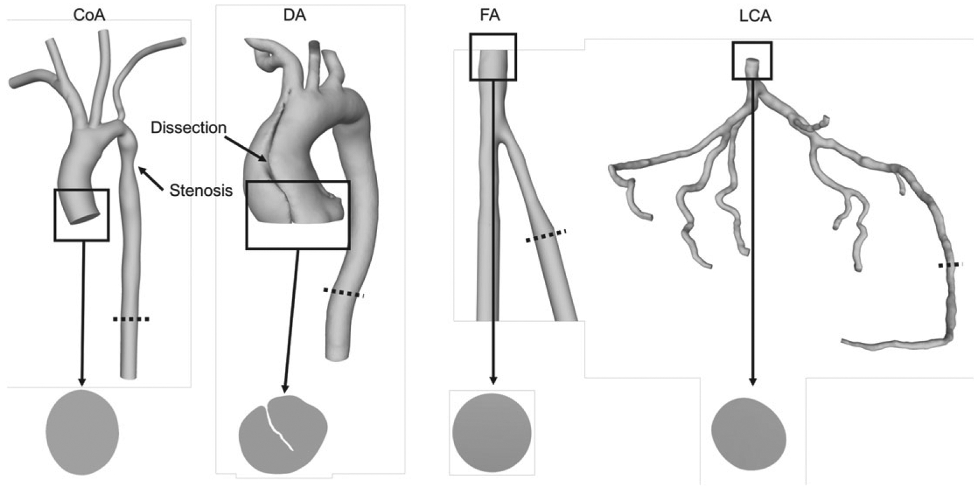
The geometries used in this study from left to right: coarctation of the aorta (CoA), dissected aorta (DA), femoral artery (FA), and left coronary artery (LCA). The inlets of each geometry are labeled. Notice the irregular inlet in the DA. The dotted lines indicate the slice locations for convergence tests (section 2.5.2)

• The CoA was derived from MRA data, has a 65% coarctation, and obtained from the Open Source Medical Software repository.³²

• The DA was derived from CTA data, segmented with Materialise Mimics, and obtained from the Department of Surgery at Duke University Hospital with appropriate institutional review board (IRB) approval.

• The FA was derived from CTA data and obtained from the OSIRIX DICOM Image Library.

• The LCA was derived from CTA data, segmented with Materialise Mimics, and obtained from Brigham and Women’s Hospital with appropriate IRB approval.

2.2 |. Lattice Boltzmann method

Blood flow was simulated with HARVEY, a massively parallel hemodynamics application.³³ HARVEY implements the LBM, a mesoscopic solver for the Navier-Stokes equations.⁴ The LBM represents fluid points with a probability distribution function f_i(x, t), denoting the likelihood that a particle is at grid point x, at time t, and traveling with discrete velocity c_i around a fixed Cartesian grid:

$$f_i\left(x+c_i,t+1\right)-f_i(x,t)=-\Omega \left(f_i(x,t)-f_i^{eq}(x,t)\right).$$ (1)

At each time step, two key processes occur: streaming and collision. During streaming, the particles travel by discrete velocities to neighboring nodes defined by the lattice discretization. In collision, the particle distribution relaxes toward the Maxwell-Boltzmann equilibrium distribution, which can be approximated with $f_i^{eq}$:

$$f_i^{eq}=w_i\rho \left(1+\frac{c_i\cdot u}{c_s^2}+\frac{uu:\left(c_i{c}_i-c_s^{2}I\right)}{2c_s^4}\right),$$ (2)

for lattice weights w_i and lattice speed of sound $c_s=\frac{1}{\sqrt{3}}$. HARVEY uses a single relaxation time Bhatnagar-Gross-Krook (BGK) collision operator³⁴:

$$\Omega \left(f,f^{eq}\right)=\omega =\frac{1}{\tau }.$$ (3)

The relaxation time τ is related to the lattice Boltzmann (LB) viscosity (ν_LB) of the fluid:

$$v_{LB}=c_s^2\left(\tau -\frac{1}{2}\right).$$ (4)

The LB viscosity is given as an input into the simulation, and the time step dt is computed with the following equation:

$$dt=\frac{v_{LB}d{x}^2}{v},$$ (5)

where ν is the kinematic viscosity and dx is the grid spacing between lattice points in physical units. Macroscopic values including fluid density ρ and velocity u are recovered from the distribution functions according to the following equations:

$$\rho =\sum _i{f}_i,$$ (6)

$$u=\frac{1}{\rho }\sum _i{c}_i{f}_i.$$ (7)

A detailed description of the LBM can be found in Krüger et al.¹⁶

HARVEY uses a standard D3Q19 lattice with uniform grid spacing and a half-way bounce-back boundary condition at the vessel walls (Figure 2). Prior to simulating flow, all variables are nondimensionalized using dt, dx, and the physical fluid density. After the simulation is complete, the nondimensional variables are redimensionalized for analysis.

FIGURE 2.

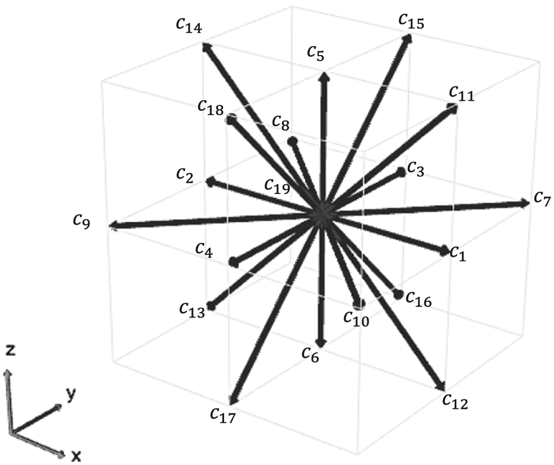
The D3Q19 lattice used in HARVEY

2.3 |. Modeling assumptions

To simplify the experimental design for this study, we assumed that vessel walls are rigid and flow is Newtonian. Rigid walls are a common assumption when modeling blood flow in vasculature.^35–37 Furthermore, based on the high shear rates in the arteries used in this work, a Newtonian assumption for blood flow is valid. Simulating blood flow in small arteries with lower shear rates often requires a non-Newtonian model, such as the Carreau-Yasuda or power law model.^38,39 Blood exhibits non-Newtonian behavior from red blood cell aggregation that typically occurs at low shear rates. A common assumption for blood flow is to assume non-Newtonian behavior at shear rates less than 100 s⁻¹, often found in distal segments of vasculature like arterioles.^40–44 All pulsatile simulations were performed for one cardiac cycle, and constant flow simulations were analyzed once steady state was achieved.

2.4 |. Inlet and outlet conditions

In this study, the ZH and FD boundary conditions were compared in the four geometries described above. The main purpose of these boundary conditions is to derive the distribution functions at each inlet and outlet when implemented as Poiseuille velocity or pressure profile. The methods described in this section pertain to straight (flat) boundaries. Here, we describe the general methods for implementing each boundary condition in HARVEY.

2.4.1 |. Implementing the Zou-He boundary condition

The fundamental idea of the Zou-He boundary condition is to solve for the unknown distributions by bounce-back of the nonequilibrium component of the distribution function.²⁹ In conjunction with a correction for the transverse momentum, this boundary condition has been generalized in a D3Q19 lattice by Hecht and Harting.³⁰ The ZH boundary condition is local in its operations and thus can be easily implemented in parallel. Additionally, it is highly accurate in simple geometries.¹⁷ However, the relaxation times for which ZH algorithms are stable is limited to low Re and may present problems in vasculature in large arteries where high Re prevail.⁴⁰

The ZH method replaces only the unknown distributions at each node; in the case of a D3Q19 lattice, there will be five unknown distributions after the streaming step. The following equation is used to calculate the unknown distributions:

$$f_{-i}=f_i-\frac{2w_i\rho }{c_s^2}\left(c_i\cdot u\right)-\frac{\rho }{3}\left(t_i\cdot u\right)+\frac{1}{2}\sum _{j=0}^{18}{f}_j\left(t_i\cdot c_j\right)\left(1-\left|c_j\cdot n\right|\right),$$ (8)

where f_i represents the distributions streaming into the boundary, f_−i denotes the bounce-back populations, c_j are the direction vectors, n is the outward normal vector, and t_i is computed as follows:

$$t_i=c_i-\left(c_i\cdot \mathit{\text{n}}\right)\mathit{\text{n}}.$$ (9)

By the continuity relation, three of the four macroscopic variables—density ρ and the three components of velocity u—in Equation 8 may be specified, while the last is computed from the distribution function. In this study, we specify the complete velocity u for inlet conditions, whereas density ρ and the transverse velocity u_|| are specified at the outlet.

2.4.2 |. Implementing the finite difference boundary condition

While originally introduced by Skordos,³¹ the FD boundary condition implementation in this study is based on Latt et al.¹⁷ In this implementation, a regularization procedure replaces all components of the distribution function, both known and unknown. This procedure requires the computation of the strain rate tensor using a finite difference scheme. As a result, the FD boundary conditions offer greater numerical stability in simple geometries, but the inherent nonlocality of the method results in an increased computational load and more complicated parallelization schemes.

Unlike the ZH method, the FD approach replaces all the distributions at each node:

$$f_i=f_i^{eq}-\rho \frac{w_i}{c_s^2\omega }{Q}_i:\mathit{\text{S}},$$ (10)

where S is the strain rate tensor defined by

$$\mathit{\text{S}}=\frac{1}{2}\left(\nabla \mathit{\text{u}}+{(\nabla \mathit{\text{u}})}^T\right),$$ (11)

and Q_i is defined by

$$Q_i=c_i{c}_i-c_s^{2}I,$$ (12)

where I is the identity matrix. Note that the : is used for a contraction between two tensors. The strain rate tensor S is calculated at each node with a finite difference method that is first order in the normal direction and second order in the tangential direction. While the strain rate tensor can be computed locally in the LBM, using velocity gradients from the neighboring nodes increases the stability of the simulation.

2.5 |. Velocity profile algorithm for irregular inlets

Applying patient-tuned boundary conditions has been shown to improve fidelity and accuracy of cardiovascular simulation parameters like helical flow patterns, wall shear stress, and pressure gradients.⁴⁵ Recently, 3D phase contrast MRI, commonly referred to as 4D MRI, has enabled the acquisition of patient-specific velocity profiles.⁴⁶ However, patient-specific inflow profiles based on 4D MRI are not typically available. Further, 4D MRI data is challenging to use in CFD simulations because of low resolutions, high signal-to-noise ratio, and diagnostic variations arising from respiratory motion, changes in heart rate, and patient position.^47,48 Thus, specifying physiological velocity conditions at the inlet is a nontrivial task, particularly in complex vascular geometries. A variety of inlet velocity conditions, such as parabolic or Womersley profiles, are employed in hemodynamic simulations.⁴⁹ Applying a physiological flow profile to the inlets of vascular geometries is straightforward if the inlets are approximately circular, as is the case in the CoA, FA, and LCA (Figure 1). To implement a parabolic flow profile in these inlets, a naive implementation would be to determine the velocity u as a function of the geometric center and radius of the inlet.

However, for an irregular inlet shape like that of the DA geometry, a more flexible notion is required for determining the location of maximum velocity. One approach would involve solving a Poisson-like equation over the surface of the inlet. However, this is a heavy solution to a problem for which an exact solution is not required. Thus, we approximate the velocity profile shape based on the local inlet topology (Figure 3). Such an adaptive approach is implemented by computing the inlet velocity at each point as a function of its distance d to the nearest wall. For an irregular inlet, the maximum velocity u_max should be assigned to the point that is farthest from its nearest wall d_max. The velocities at the remaining points are described by the following equation:

$$\mathit{\text{u}}={\mathit{\text{u}}}_{\max }-{\mathit{\text{u}}}_{\max }{\left(1-\frac{d}{d_{\mathit{\text{max}}}}\right)}^2.$$ (13)

FIGURE 3.

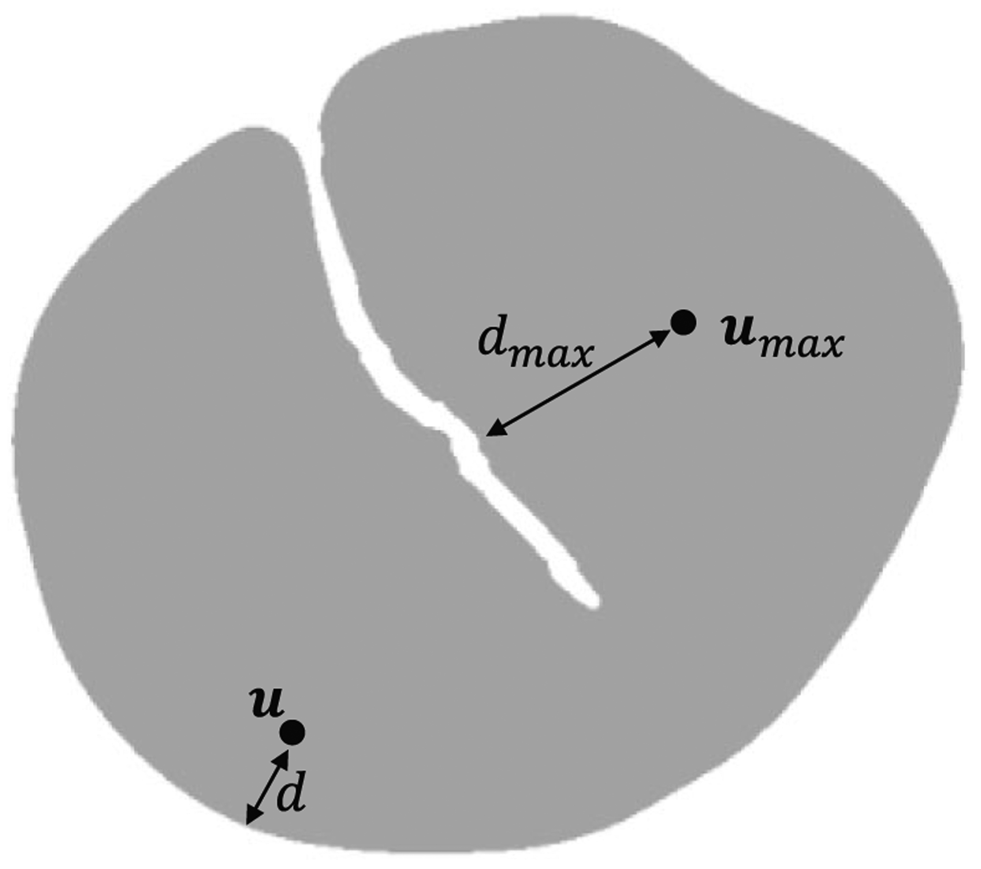
A new velocity profile algorithm was developed for the inlet of the DA. The point depicted by u_max describes the point farthest from its nearest wall. The distance between this point and its nearest wall is d_max, and we assign it a velocity of u_max. The velocity u of the second point in this figure is computed based on its distance d from the nearest wall. This point represents any arbitrary point on the inlet

This algorithm does not require circular inlets, allowing the computation of an accurate velocity profile for diseased vasculature with complex inlets. In the case of circular inlet, d_max is equal to the radius.

In parallel implementations, the inlet points may be stored on many different processors, and each point’s nearest wall point can also be on a separate processor. Additionally, the point at d_max will only be available to other points on its own processor. To solve these problems, Message Passing Interface (MPI) collectives were used to communicate the locations of the wall points and d_max to each processor owning points on the boundary. The time complexity of our algorithm is O(MN) where M is the number of wall points at the inlet and N is the number of inlet points. Solving a Poisson equation over a rectangular 2D domain with a fast Fourier transform has a time complexity of O(NlogN). However, this algorithm is computed only once before the simulation, so runtime is not a critical factor. Instead, we note that the advantage of our algorithm is that we avoid the unnecessary implementation of a parallel Poisson-like solver.

To demonstrate the usefulness and validate the novel adaptive inlet velocity profile algorithm, we performed three set of numerical tests. First, we applied the algorithm to the DA where the inlet geometry is irregular. Figure 4 shows the inlet velocity profile in the DA. In contrast to the naive implementation, we were able to retrieve the no-slip boundary conditions at the wall and a parabolic profile with maximum velocity at the point farthest from any wall.

FIGURE 4.

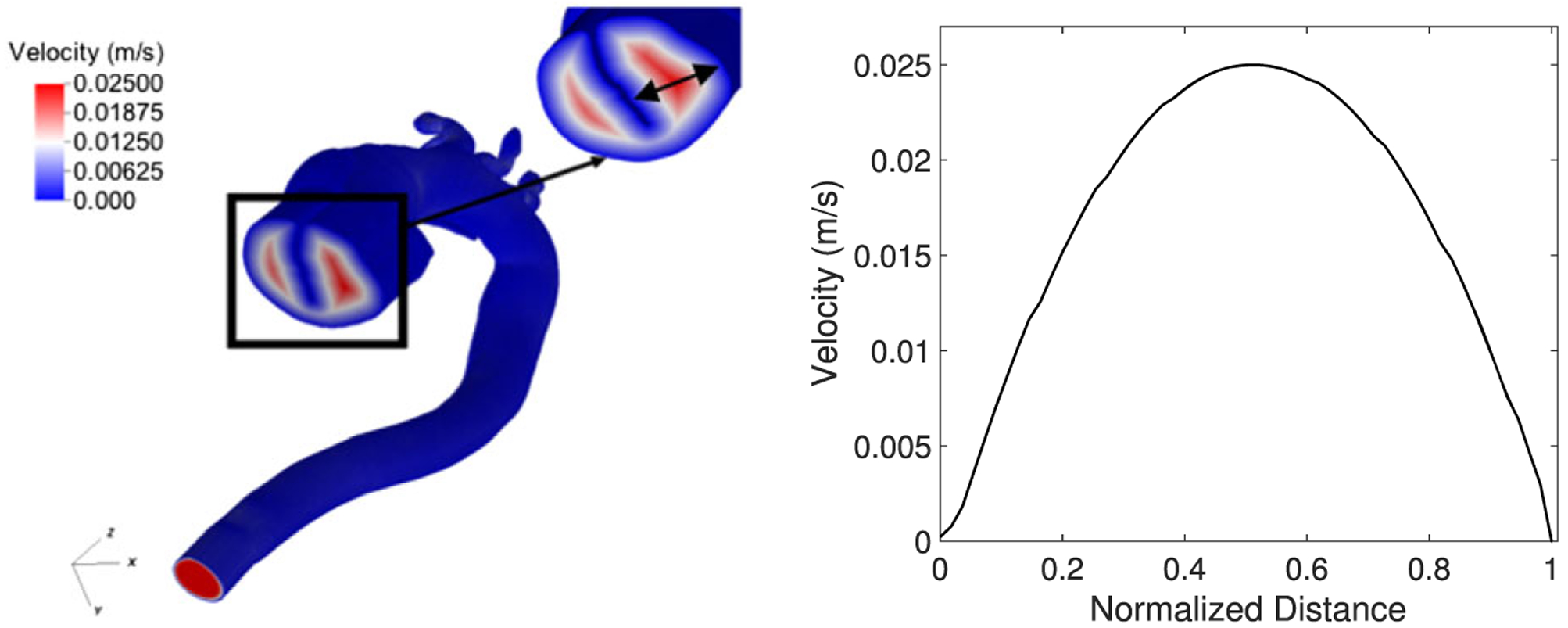
The inlet velocity algorithm applied to the dissected aorta (DA) with tear in the center. The plot on the right shows the parabolic velocity profile along the DA inlet

In our second test, we simulated flow through a pipe and compared the results using the adaptive approach with the naive implementation in HARVEY by computing the relative error E at slices along the geometry. For the set of lattice points i in the slice, the relative error E of the velocity profile along a slice was computed with the following equation:

$$E=\sqrt{\frac{\sum _i{\left({\mathit{\text{u}}}_i^r-{\mathit{\text{u}}}_i\right)}^2}{\sum _i{\left({\mathit{\text{u}}}_i^r\right)}^2}},$$ (14)

where u and u^r are the current and reference velocities, respectively.^50,51 The naive implementation was previously validated by comparing simulated flow with experimental flow through 3D printed vasculature using particle image velocimetry (PIV).²⁵ Results showed that flow through the pipe in the two implementations was nearly identical (error E < 1.0e-10). Finally, to ensure the algorithm was implemented correctly in parallel, velocity profiles in the pipe were compared between simulations with one, two, four, and eight processors where the simulation with one processor was used as the reference for error computation. Results show that the velocity profiles were identical for any number of processors (error E < 1.0e-10), thus validating the parallel implementation specifically when the inlet area was split on different processors.

3 |. NUMERICAL RESULTS

Blood flow was simulated in a CoA, DA, FA, and LCA using the ZH and FD inlet and outlet boundary conditions. In each simulation, the same type of boundary condition was applied at the inlet and outlets. The ZH and FD boundary conditions were evaluated by computing their influence on accuracy, numerical convergence, numerical stability, and computational performance in the vascular geometry. For most of the simulations, blood was assumed to have dynamic viscosity 4 cP and physical density 1060 kg/m³.⁵² However, when comparing results with in vitro experiments, the viscosity was set to 2.05 cP with an inlet velocity of 7.6 cm/s to match the experimental parameters. All simulations were performed with Intel Xeon E5–2699V4 processors and 56 Gb/s Infiniband interconnect on the Duke Compute Cluster.

3.1 |. Numerical stability

Numerical stability is necessary to obtain usable simulation results. An LBM simulation is said to be stable if the total variation of the distribution function from the equilibrium distribution remains bounded.¹⁸ Because blood flow simulations often require significant computational resources, stability testing is also important to determine the lowest resolution possible while maintaining a stable and convergent simulation. Many studies have focused on the stability of the LBM method, while neglecting the impacts of boundary conditions.^18,19 Other groups studied the LBM in idealized geometries for benchmark flows and demonstrated that numerical stability is strongly dependent on the boundary conditions.^17,20 However, it is not currently known how the stability of complex image-derived simulations compares with idealized benchmark models. We predicted that stability would differ significantly from idealized models at the inlets and outlets due to complex inlet and outlet geometries and physiological flow profiles. These differences arise from anatomic variations such as curved boundaries, vessel tortuosity, and branching patterns in addition to time-varying pulsatile flows. In this section, we assess the influence of inlet and outlet conditions on the stability of simulations in complex vascular geometries.

To determine stability for the ZH and FD, flow was simulated in each geometry over a range of resolutions with steady and pulsatile flow. The pulsatile flow waveform used in each geometry was based on the aorta inflow waveform provided by Figuero et al.⁵³ In this study, resolution is defined as the number of grid points across the diameter of the inlet. The maximum Re at the inlet that produced a stable simulation for a given geometry and resolution was recorded. For pulsatile flow, the waveform was scaled based on the desired Re. For a given geometry, the LB viscosity was held constant over all resolutions considered. Further, for steady flow simulations, the LB velocity was set to 0.075 at the lowest grid resolutions for each geometry to minimize compressibility effects.¹⁷

Results from the stability analysis are depicted in Figure 5. In all four geometries, the FD condition demonstrated stability at significantly higher Re than the ZH condition. Beyond a certain resolution, the maximum stable Re for the ZH condition increased only modestly. Conversely, the stability region increased more significantly for the FD condition at high resolutions. Interestingly, the stability differences between pulsatile and steady flow depended on the geometry: In the CoA and LCA, steady flow was more stable, but an opposite trend occurred in the DA and FA.

FIGURE 5.

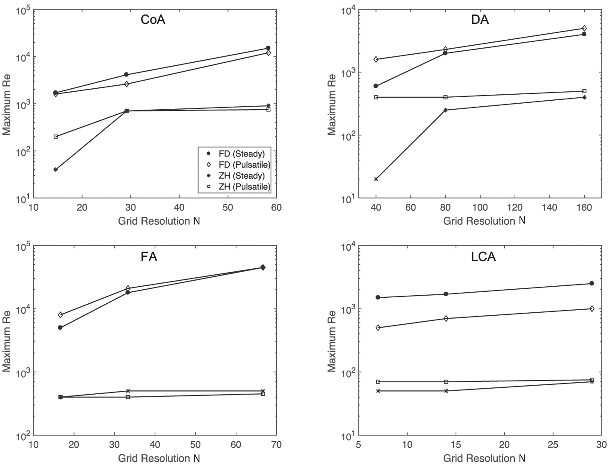
Stability analysis for coarctation of the aorta (top left), dissected aorta (top right), femoral artery (bottom left), and left coronary arteries (bottom right). Figures depict maximum stable Re as a function of grid resolution, where grid resolution is defined as the number of grid points across the diameter of the inlet. Note that the dissected aorta (DA) is significantly larger than the coarctation of the aorta (CoA) geometry explaining the higher grid resolutions in the DA

3.2 |. Convergence

Temporal and spatial convergence rates for blood flow simulations are important to reach the solution in a reasonable time. Temporal convergence ensures that we reach steady state starting from quiescent flow. Spatial convergence provides a mesh-independent solution, which we can achieve by refining the grid until the discretization error asymptotically decreases to zero. Specifically, by analyzing and comparing the grid convergence, we can estimate the order of accuracy and whether that is influenced by either of the boundary conditions in complex geometries. In idealized geometries, the ZH and FD conditions were found to have similar second-order rates of spatial convergence, but the ZH condition was more accurate at a given resolution in some instances.¹⁷ However, in complex, image-derived, vascular geometries, whose flow results are strongly influenced by boundary conditions, it is difficult to demonstrate numerical convergence.⁵⁴ In this section, we assess the influence of inlet and outlet conditions on the temporal and spatial convergence of simulations in the CoA, FA, and LCA. Since flow regimes in CoA and DA are similar, the DA was omitted from this study. For the sake of simplicity, we restrict this comparison to steady flow.

As flow in complex geometries does not have an analytical solution, we used a high-resolution grid as the reference solution for spatial convergence and a long simulation for temporal convergence. A physical resolution of 50μm was used as the reference for each geometry, corresponding to 135, 63, and 53 grid points across the inlets of the CoA, FA, and LCA, respectively. Error, computed with Equation 14, is measured over a cross-sectional slice of each geometry, corresponding to the dotted lines in Figure 1. The simulation duration determined from the temporal convergence test was subsequently used as the duration of the spatial convergence test. To ensure a clear comparison, the Re and LB viscosity were kept constant between numerical tests with a given inlet and outlet condition. The corresponding values of Re and τ can be found in Table 2 for each geometry.

TABLE 2.

Example simulations representing 1 second of total time

		Tau		Grid Resolution N		Time Steps		Run Time, s
	Re	FD	ZH	FD	ZH	FD	ZH	FD	ZH
CoA	675.0	0.508	0.575	17	135	2564	16 000	4.98	7204.30
FA	157.5	0.508	0.575	11	63	5102	16 660	23.47	561.02
LCA	105.6	0.508	0.575	11	53	27 778	64 000	25.16	4626.83

Simulations using the ZH boundary condition require a higher relaxation time τ, grid resolution, and number of time steps. Average Re values over a cardiac cycle were chosen.

Results for temporal and spatial convergence are shown in Figures 6 and 7, respectively. All simulations had small errors, on the order of 0.01, at longer times scales and higher grid resolutions. In the LCA, a smaller geometry, there were no significant convergence differences between simulations using the ZH and FD method. However, in the CoA and FA, results demonstrate that the ZH and FD method converged with different relative error for both spatial and temporal convergence. In spatial convergence tests, the order of accuracy lies between first and second order.

FIGURE 6.

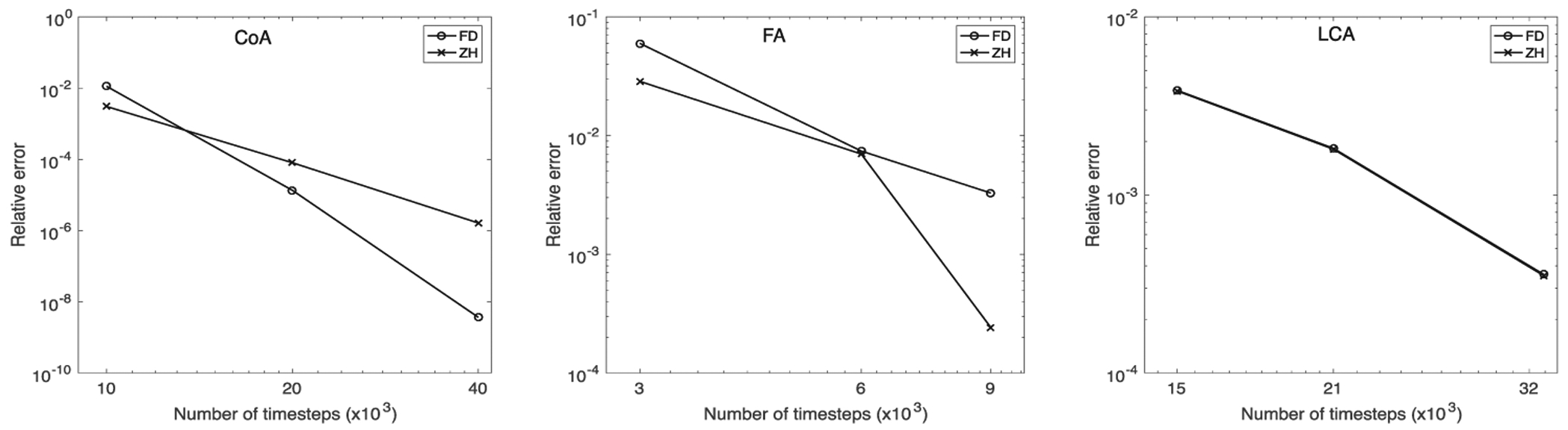
Temporal convergence for (left to right) coarctation of the aorta (CoA), femoral artery (FA), and left coronary artery (LCA)

FIGURE 7.

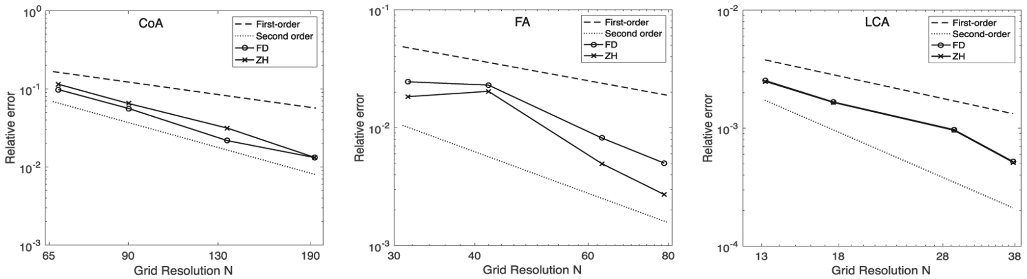
Spatial convergence for (left to right) coarctation of the aorta (CoA), femoral artery (FA), and left coronary artery (LCA)

3.3 |. Experimental validation

CFD simulations approximate analytical solutions and include errors resulting from discretization, iteration, and modeling.⁵⁴ However, vascular flow is complex, and analytic solutions often do not exist. To address this challenge, we 3D printed the FA and used PIV to compare experimental and simulated hemodynamics; 3D printing allows for an accurate physical representation of the geometry while providing a controllable environment with known and easily tunable parameters. The experimental setup that we used for this work was previously described in detail by Gounley et al.²⁵ We initially chose to use the FA and CoA for experimental comparison because we were interested in comparing geometries with high Re, often leading to more complex flow patterns. However, stability results in the preceding section demonstrated that the ZH boundary condition was unstable at the Re necessary for flow in the CoA. Thus, PIV comparisons were only performed for the ZH and FD boundary conditions in the FA.

In these simulations, relative error was calculated with respect to PIV results. Velocity magnitude u was recorded at the vessel bifurcation as indicated by the line depicted in Figure 8. Temporal and spatial convergence results are shown in Figure 8. ZH and FD boundary conditions demonstrated similar spatial and temporal convergence. Results showed that the relative error for temporal and spatial convergence was between 0.01 and 0.1. This could result from minor differences in the PIV setup and CFD simulations, particularly at the outlet boundary conditions and inherent error resulting from 3D printing. Thus, we note similar accuracy between the ZH and FD boundary conditions.

FIGURE 8.

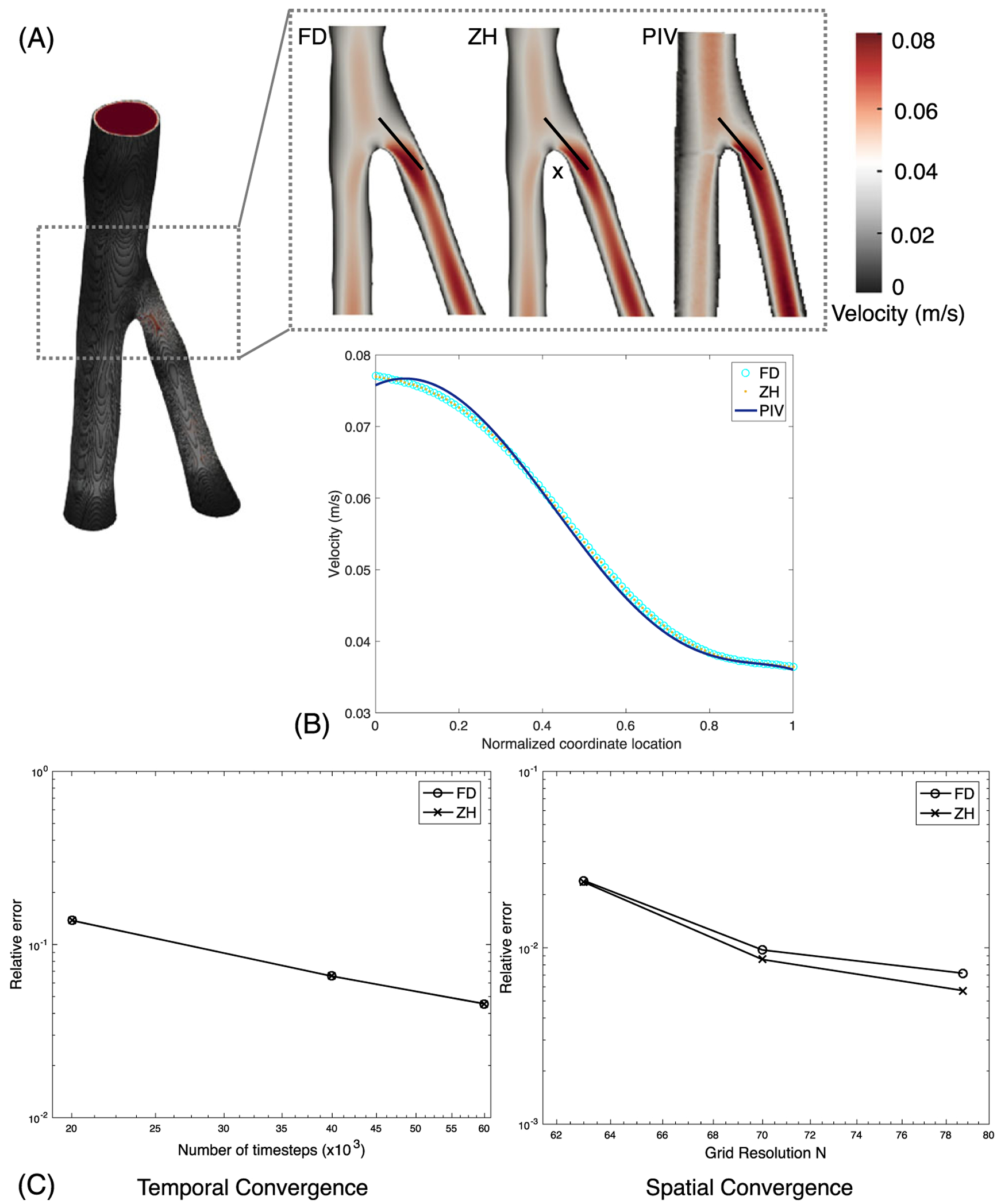
Computational fluid dynamics (CFD)–particle image velocimetry (PIV) comparison: A, the femoral artery (FA) with slices for each boundary condition. B, The magnitude of velocity was plotted along the black lines shown in the slices. C, The temporal and spatial convergence analyzed with respect to the in vitro PIV-measured velocity profile

3.4 |. Computational performance

For a given number of time steps and grid resolution, the overall simulation run times are generally not influenced by the inlet and outlet boundary conditions, as the inlets and outlets comprise only a small percentage of the total volume. This was confirmed with strong and weak scaling tests (data not shown). Therefore, the run times exclusively at the inlets and outlets were computed in each geometry. For a given geometry, the resolution and number of time steps were held constant between simulations using the ZH and FD method. All simulations for these tests were performed with one processor. As demonstrated in Table 1, the percentage of run time spent at the inlets and outlets is less than 0.5%.

TABLE 1.

The combined run times at the inlets and outlets were computed as a percentage of the total tun times

Present of Total Run Time
BC	CoA	FA	LCA
FD	0.47%	0.17%	0.28%
ZH	0.19%	0.068%	0.14%

Additionally, overall run time comparisons were performed with physiological Re. Blood flow was simulated for a physical time of one second. As indicated by the stability plots (Figure 5), the FD method is significantly more stable than ZH leading to large differences in grid resolution. However, the ZH method also needed a higher relaxation time τ, which increased Δt according to Equations 3 and 4. Both of these factors were considered when choosing the number of steps corresponding to a physical time of 1 second. Table 2 summarizes the runtime results. The ZH method run times were approximately three orders of magnitude higher than FD method for the CoA and FA and approximately two orders of magnitude higher for the LCA.

4 |. DISCUSSION

Our main objective in this study was to evaluate ZH and FD boundary conditions to determine their suitability when simulating blood flow in image-derived vasculature using the LBM. The LBM is an attractive approach for blood flow simulations as it is easily parallelized and implemented in complex geometries. Additionally, the LBM is becoming heavily used for hemodynamics, and thus, it is important to understand the stability and computational trade-offs of different boundary condition for physiological cases. While there are other boundary conditions, as described in Latt et al¹⁷ and Nash et al,²⁰ here we restrict our comparison with the ZH^29,30 and FD^17,31 schemes, since the purpose of this study is to facilitate implementation of the LBM in patient geometries across different scales. Further, boundary conditions in the LBM are broadly categorized based on the treatment of particle populations on the boundary node by replacing either all or only the unknown particle populations.¹⁷ The FD and ZH schemes are representative of these two categories, as described in Section 2.4. Although the FD and ZH boundary conditions have been compared in simple geometries, we have not found any work extensively comparing these two schemes in complex arterial vasculature.^17,20

Four image-derived geometries, representing diseased and healthy vasculature were used in this work: a CoA, FA, DA, and LCA. Both boundary conditions were compared in each geometry with respect to stability, convergence, accuracy, and computational performance, all common and important metrics when evaluating numerical algorithms. The main purpose of this work is to serve as a guide to researchers to determine which boundary conditions to use when simulating blood flow with the LBM.

4.1 |. Numerical stability, convergence, and run times are key factors that help distinguish Zou-He and finite difference boundary conditions

The numerical stability of ZH and FD boundary conditions was compared in the CoA, DA, FA, and LCA. Results showed that the ZH boundary condition is significantly less stable than FD in all geometries, agreeing with previous studies that tested stability in simple geometries under idealized settings.¹⁷ In particular, Latt et al¹⁷ showed that the FD method could be used to simulate flows with Re nearly two orders of magnitude higher than the ZH method.

When increasing the Re with ZH boundary conditions, instabilities began to arise first at the inlets and outlets. However, with the FD boundary condition, instabilities at high Re originated in narrow sections of the blood vessel. Thus, when using the ZH method, the stability limit was imposed by the inlet and outlet boundary conditions. In contrast, the stability limit for the FD method was imposed by other simulation parameters such as the BGK collision operator or the wall boundary condition. At the narrow sections of blood vessels, greater instabilities in the LBM arise because of the increase in local Re and Mach number. The half-way bounce-back boundary condition at the wall is likely the origin of the instabilities at high Re in narrow sections.²¹ Peak flow rates for steady and pulsatile flow were the same resulting in similar stability. The Re that can reasonably be achieved using the ZH boundary is significantly lower than typical Re for many of the major arteries. For example, the Re in the aorta and FA can reach over 10 000 and 1000, respectively.⁴⁰ High Re can also arise in physiological conditions such as hyperemia or the state of maximum vasodilation, which is important to noninvasively compute diagnostic metrics such as fractional flow reserve.² These values are achievable using the FD method but generally not with the ZH method at similar grid resolutions. At high resolutions, the ZH method could be used in small blood vessels with lower Re. For example, the coronary and middle cerebral arteries can have Re less than 200 and 100, respectively, and may be well suited for the ZH method.^55,56 Similarly, Re in microcapillary networks typically lies between 1 and 10. However, in these flow regimes, a non-Newtonian model may be necessary.⁵⁷

Convergence of FD and ZH boundary conditions was similar in each geometry tested. Our results showed similar convergence rates for all geometries tested with ZH and FD methods. Latt et al¹⁷ showed second-order convergence in an idealized setting, but we see a slightly lower convergence likely due to the complexity of the geometries, leading to first-order convergence of the half-way bounce-back boundary conditions at the walls. While we exclusively used half-way bounce-back boundary conditions for this study, we note that a full-way bounce-back scheme at the walls is first-order accurate in idealized geometries and unlikely to improve convergence.⁵⁸ Additionally, the overall errors were similar between the FD and ZH boundary conditions but differed between geometries (Figures 6 and 7). The variable errors between geometries are not surprising as each geometry is complex and different in both shape and size. Errors in the CoA and FA had higher variation than the LCA possibly due to higher Re and more complex flow patterns. While convergence tests showed that our simulations approached high-resolution reference solutions, experimental validation was also important to show that results agree with in vitro or in vivo flow. In vitro blood flow experiments were performed with 3D printed vasculature using PIV, as in vivo velocities and pressures were not available. The FA and CoA were optimal choices for experimental comparisons because of their high Re. However, the ZH method was consistently unstable under physiological Re in the CoA. Therefore, only the FA was used for in vitro comparisons. The particular velocity profile line used for the comparisons was chosen near the bifurcation in the FA where flow patterns are known to be complex. Both FD and ZH boundary conditions showed similar accuracies in the FA (Figure 8).

The third distinguishing factor, run time, was highly variable between ZH and FD boundary conditions. Initially, we computed run times exclusively at the inlets and outlets of each geometry. All parameters were held constant between FD and ZH simulations. In Table 1, we showed that the inlet and outlet run times comprise only a small fraction of the total runtime, although the FD method consumed a greater percentage of the total runtime in every geometry. This result is expected for physiological flows. The runtimes needed for accurate simulations are highly dependent on the stability of the boundary condition. To analyze overall runtimes, blood flow was simulated with the FD and ZH methods using the same Re for a physiological time of 1 second. The ZH method was less stable and therefore required a higher relaxation time τ, grid resolution, and number of time steps to achieve the same physiological time. The runtimes in each geometry were nearly three orders of magnitude larger with the ZH method as compared with the FD method. This result is an important distinguishing factor that clearly demonstrates the strength of the FD method in imaged-derived vasculature with high Re flows. While the time spent in boundary conditions themselves is longer for the FD method, the run time is significantly reduced overall because of lower resolutions.

4.2 |. Conclusions and recommendations

The ZH and FD inlet and outlet boundary conditions used in the LBM were compared and evaluated in image-derived vasculatures. Comparisons included numerical stability, numerical convergence, accuracy, and run-time. Each of these factors is important in clinical applications to achieve fast and accurate simulations. To summarize our findings, we offer recommendations here as to which boundary condition to use when simulating blood flow. The main differences between simulations using the ZH and FD boundary conditions were stability and runtime, as convergence generally showed similar results. The FD method offered greater numerical stability, particularly at high Re, and significantly decreased runtime (Figure 5, Table 2). Simulating flow at high Re is important in large arteries. Based on the stability plots, the FD boundary condition can simulate flow throughout all of the major arteries, including the aorta that contains the highest Re flows. However, simulations using the ZH method would only be sufficiently stable in small vasculature, with an increased runtime.

The FD method is a better choice to simulate blood flow in image-derived vasculature, particularly in large arteries, but the ZH method may be simpler to implement in parallel as all of the calculations are local (section 2.3.1). While, the ZH method was shown to have greater accuracy in idealized conditions, such as two-dimensional channel flow,¹⁷ we conclude that it may not be well suited for flow in large arteries. Overall, this study is intended to serve as a guide to researchers interested in using the LBM for physiological blood flow simulations.

REFERENCES

- 1.Marsden A Optimization in cardiovascular modeling. Annu Rev Fluid Mech. 2014;46:519–546. [Google Scholar]
- 2.Taylor CA, Fonte TA, Min JK. Computational fluid dynamics applied to cardiac computed tomography for noninvasive quantification of fractional flow reserve. J Am Coll Cardiol. 2013;61(22):2233–2241. [DOI] [PubMed] [Google Scholar]
- 3.Aidun CK, Clausen JR. Lattice-Boltzmann method for complex flows. Annu Rev Fluid Mech. 2010;42:439–472. [Google Scholar]
- 4.Chen S, Doolen GD. Lattice Boltzmann method for fluid flows. Annu Rev Fluid Mech. 1998;30(1):329–364. [Google Scholar]
- 5.Mazzeo MD, Coveney PV. Hemelb: A high performance parallel lattice-Boltzmann code for large scale fluid flow in complex geometries. Comput Phys Commun. 2008;178(12):894–914. [Google Scholar]
- 6.Donath S, Götz J, Bergler S, Feichtinger C, Iglberger K, Rüde U. waLBerla: The need for large-scale super computers In: High Performance Computing in Science and Engineering. Garching/Munich, Germany: 2007; 2009:459–473. [Google Scholar]
- 7.Randles A, Draeger EW, Oppelstrup T, Krauss L, Gunnels JA. Massively parallel models of the human circulatory system In: Proceedings of the International Conference for High Performance Computing, Networking, Storage and Analysis. Austin, TX, USA; 2015:1–11. [Google Scholar]
- 8.Hirabayashi M, Ohta M, Rüfenacht DA, Chopard B. A lattice Boltzmann study of blood flow in stented aneurism. Future Gener Comput Syst. 2004;20(6):925–934. [Google Scholar]
- 9.Harrison S, Smith S, Bernsdorf J, Hose D, Lawford P. Application and validation of the lattice Boltzmann method for modelling flow-related clotting. J Biomech. 2007;40(13):3023–3028. [DOI] [PubMed] [Google Scholar]
- 10.Patronis A, Richardson RA, Schmieschek S, Wylie BJ, Nash RW, Coveney PV. Modelling patient-specific magnetic drug targeting within the intracranial vasculature. Front Physiol. 2018;9:331. [DOI] [PMC free article] [PubMed] [Google Scholar]
- 11.Bernabeu MO, Jones ML, Nielsen JH, et al. Computer simulations reveal complex distribution of haemodynamic forces in a mouse retina model of angiogenesis. J R Soc Interface. 2014;11(99):20140543. [DOI] [PMC free article] [PubMed] [Google Scholar]
- 12.Gounley J, Draeger EW, Randles A. Numerical simulation of a compound capsule in a constricted microchannel. Procedia Comput Sci. 2017;108:175–184. [DOI] [PMC free article] [PubMed] [Google Scholar]
- 13.Balossino R, Pennati G, Migliavacca F, et al. Computational models to predict stenosis growth in carotid arteries: which is the role of boundary conditions? Comput Methods Biomech Biomed Eng. 2009;12(1):113–123. [DOI] [PubMed] [Google Scholar]
- 14.Vignon-Clementel IE, Figueroa CA, Jansen KE, Taylor CA. Outflow boundary conditions for three-dimensional finite element modeling of blood flow and pressure in arteries. Comput Methods Appl Mech Eng. 2006;195(29):3776–3796. [Google Scholar]
- 15.Zamir M The physics of pulsatile flow; 2000. [Google Scholar]
- 16.Krüger T, Kusumaatmaja H, Kuzmin A, Shardt O, Silva G, Viggen EM. The Lattice Boltzmann Method. Cham, Switzerland: Springer; 2017. [Google Scholar]
- 17.Latt J, Chopard B, Malaspinas O, Deville M, Michler A. Straight velocity boundaries in the lattice Boltzmann method. Phys Rev E. 2008;77(5):056703. [DOI] [PubMed] [Google Scholar]
- 18.Sterling JD, Chen S. Stability analysis of lattice Boltzmann methods. J Comput Phys. 1996;123(1):196–206. [Google Scholar]
- 19.Bouzidi M, D’Humieres D, Lallemand P, Luo L-S. Lattice Boltzmann equation on a 2D rectangular grid In: Institute for Computer Applications in Science and Engineering; 2002; Hampton VA. [Google Scholar]
- 20.Nash RW, Carver HB, Bernabeu MO, et al. Choice of boundary condition for lattice-Boltzmann simulation of moderate-Reynolds-number flow in complex domains. Phys Rev E. 2014;89(2):023303. [DOI] [PubMed] [Google Scholar]
- 21.Hegele LJr, Scagliarini A, Sbragaglia M, et al. High-Reynolds-number turbulent cavity flow using the lattice Boltzmann method. Phys Rev E. 2018;98(4):043302. [Google Scholar]
- 22.Artoli AM, Hoekstra AG, Sloot PM. Mesoscopic simulations of systolic flow in the human abdominal aorta. J Biomech. 2006;39(5):873–884. [DOI] [PubMed] [Google Scholar]
- 23.Melchionna S, Kaxiras E, Bernaschi M, Succi S. Endothelial shear stress from large-scale blood flow simulations. Philos Trans A Math Phys Eng Sci. 2011;369(1944):2354–2361. [DOI] [PubMed] [Google Scholar]
- 24.Henn T, Heuveline V, Krause MJ, Ritterbusch S. Aortic coarctation simulation based on the lattice Boltzmann method: benchmark results In: Statistical Atlases and Computational Models of the Heart. Nice, France; 2012:34–43. [Google Scholar]
- 25.Gounley J, Chaudhury R, Vardhan M, et al. Does the degree of coarctation of the aorta influence wall shear stress focal heterogeneity? In: 2016 IEEE 38th Annual International Conference of the IEEE Engineering in Medicine and Biology Society. Orlando, FL, USA; 2016:3429–3432. [DOI] [PMC free article] [PubMed] [Google Scholar]
- 26.Boyd J, Buick J, Cosgrove J, Stansell P. Application of the lattice Boltzmann method to arterial flow simulation: investigation of boundary conditions for complex arterial geometries. Australas Phys Eng Sci Med. 2004;27(4):207–212. [DOI] [PubMed] [Google Scholar]
- 27.Zhang J, Kwok DY. Pressure boundary condition of the lattice Boltzmann method for fully developed periodic flows. Phys Rev E. 2006;73(4):047702. [DOI] [PubMed] [Google Scholar]
- 28.Kadri OE, Williams CIII, Sikavitsas g, Voronov RS. Numerical accuracy comparison of two boundary conditions commonly used to approximate shear stress distributions in tissue engineering scaffolds cultured under flow perfusion. Int J Numer Method Biomed Eng. 2018;34(11):e3132 10.1002/cnm.3132 [DOI] [PubMed] [Google Scholar]
- 29.Zou Q, He X. On pressure and velocity boundary conditions for the lattice Boltzmann BGK model. Phys Fluids. 1997;9(6):1591–1598. [Google Scholar]
- 30.Hecht M, Harting J. Implementation of on-site velocity boundary conditions for D3Q19 lattice Boltzmann simulations. J Stat Mech Theory Exp. 2010;2010(01):P01018. [Google Scholar]
- 31.Skordos P. Initial and boundary conditions for the lattice Boltzmann method. Phys Rev E. 1993;48(6):4823. [DOI] [PubMed] [Google Scholar]
- 32.Wilson NM, Ortiz AK, Johnson AB. The vascular model repository: a public resource of medical imaging data and blood flow simulation results. J Med Device. 2013;7(4):040923. [DOI] [PMC free article] [PubMed] [Google Scholar]
- 33.Randles AP, Kale V, Hammond J, Gropp W, Kaxiras E. Performance analysis of the lattice Boltzmann model beyond Navier-Stokes In: 2013. IEEE 27th International Symposium on Parallel and Distributed Processing. Boston, MA, USA; 2013:1063–1074. [Google Scholar]
- 34.Bhatnagar PL, Gross EP, Krook M. A model for collision processes in gases. I. Small amplitude processes in charged and neutral one-component systems. Phys Rev. 1954;94(3):511. [Google Scholar]
- 35.Wood NB, Weston SJ, Kilner PJ, Gosman AD, Firmin DN. Combined MR imaging and CFD simulation of flow in the human descending aorta. J Magn Reson Imaging. 2001;13(5):699–713. [DOI] [PubMed] [Google Scholar]
- 36.Soudah E, Ng EY, Loong T, Bordone M, Pua U, Narayanan S. CFD modelling of abdominal aortic aneurysm on hemodynamic loads using a realistic geometry with CT. Comput Math Methods Med. 2013; Article ID: 472564, 9 pages. [DOI] [PMC free article] [PubMed] [Google Scholar]
- 37.Papathanasopoulou P, Zhao S, Köhler U, et al. MRI measurement of time-resolved wall shear stress vectors in a carotid bifurcation model, and comparison with CFD predictions. J Magn Reson Imaging. 2003;17(2):153–162. [DOI] [PubMed] [Google Scholar]
- 38.Carreau PJ. Rheological equations from molecular network theories. Trans Soc Rheol. 1972;16(1):99–127. [Google Scholar]
- 39.Yasuda K Investigation of the analogies between viscometric and linear viscoelastic properties of polystyrene fluids. Massachusetts Institute of Technology; 1979. [Google Scholar]
- 40.Stein PD, Sabbah HN. Turbulent blood flow in the ascending aorta of humans with normal and diseased aortic valves. Circ Res. 1976;39(1):58–65. [DOI] [PubMed] [Google Scholar]
- 41.Vlachopoulos C, O’Rourke M, Nichols WW. Mcdonald’s Blood Flow in Arteries: Theoretical, Experimental and Clinical Principles. Boca Raton, FL, USA: CRC press; 2011. [Google Scholar]
- 42.Fukada E, Kaibara M. Viscoelastic study of aggregation of red blood cells. Biorheology. 1980;17(1–2):177–182. [DOI] [PubMed] [Google Scholar]
- 43.Sochi T Non-Newtonian rheology in blood circulation. arXiv preprint arXiv:13062067; 2013. [Google Scholar]
- 44.Sriram K, Intaglietta M, Tartakovsky DM. Non-Newtonian flow of blood in arterioles: consequences for wall shear stress measurements. Microcirculation. 2014;21(7):628–639. [DOI] [PMC free article] [PubMed] [Google Scholar]
- 45.Goubergrits L, Mevert R, Yevtushenko P, et al. The impact of MRI-based inflow for the hemodynamic evaluation of aortic coarctation. Ann Biomed Eng. 2013;41(12):2575–2587. [DOI] [PubMed] [Google Scholar]
- 46.Nordmeyer S, Riesenkampff E, Messroghli D, et al. Four-dimensional velocity-encoded magnetic resonance imaging improves blood flow quantification in patients with complex accelerated flow. J Magn Reson Imaging. 2013;37(1):208–216. [DOI] [PubMed] [Google Scholar]
- 47.Bruening J, Hellmeier F, Yevtushenko P, et al. Impact of patient-specific LVOT inflow profiles on aortic valve prosthesis and ascending aorta hemodynamics. J Comput Sci. 2017. [Google Scholar]
- 48.Callaghan FM, Grieve SM. Spatial resolution and velocity field improvement of 4D-flow MRI. Magn Reson Med. 2017;78(5):1959–1968. [DOI] [PubMed] [Google Scholar]
- 49.Hardman D, Semple SI, Richards JMJ, Hoskins PR. Comparison of patient-specific inlet boundary conditions in the numerical modelling of blood flow in abdominal aortic aneurysm disease. Int J Numer Method Biomed Eng. 2013;29(2):165–178. [DOI] [PubMed] [Google Scholar]
- 50.Montessori A, Falcucci G, Prestininzi P, La Rocca M, Succi S. Regularized lattice Bhatnagar-Gross-Krook model for two- and three-dimensional cavity flow simulations. Phys Rev E. 2014;89(5):053317. [DOI] [PubMed] [Google Scholar]
- 51.Hegele LA Jr, Mattila K, Philippi PC. Rectangular lattice-Boltzmann schemes with BGK-collision operator. J Sci Comput. 2013;56(2):230–242. [Google Scholar]
- 52.Kim HJ, Vignon-Clementel IE, Coogan JR, Figueroa CA, Jansen KE, Taylor CA. Patient-specific modeling of blood flow and pressure in human coronary arteries. Ann Biomed Eng. 2010;38(10):3195–3209. [DOI] [PubMed] [Google Scholar]
- 53.Alberto F, Mansi T, Sharma P, Nathan W. CFD challenge: simulation of hemodynamics in a patient-specific aortic coarctation model; 2012. [Google Scholar]
- 54.Ferziger JH, Peric M. Computational Methods for Fluid Dynamics. Berlin, Germany: Springer Science & Business Media; 2012. [Google Scholar]
- 55.Kajiya F, Tomonaga G, Tsujioka K, Ogasawara Y, Nishihara H. Evaluation of local blood flow velocity in proximal and distal coronary arteries by laser Doppler method. J Biomech Eng. 1985;107(1):10–15. [DOI] [PubMed] [Google Scholar]
- 56.Demirkaya S, Uluc K, Bek S, Vural O. Normal blood flow velocities of basal cerebral arteries decrease with advancing age: a transcranial Doppler sonography study. TJEM. 2008;214(2):145–149. [DOI] [PubMed] [Google Scholar]
- 57.Pindera MZ, Ding H, Athavale MM, Chen Z. Accuracy of 1D microvascular flow models in the limit of low Reynolds numbers. Microvascular Res. 2009;77(3):273–280. [DOI] [PubMed] [Google Scholar]
- 58.He X, Luo L-S. Theory of the lattice Boltzmann method: from the Boltzmann equation to the lattice Boltzmann equation. Phys Rev E. 1997;56(6):6811. [Google Scholar]