

Abstract
The purpose of this article is to report the inter- and intra-observer reliability of a computerized objective technique to quantify patient-specific acetabular morphology. We describe the use of and provide the software code for a technique to better define the location and magnitude of acetabular pathology. We have developed software code that allows the end user to obtain detailed measurements of the acetabulum using traditional computed tomography data. We provide the code and detailed instructions on how to use it in this article. The methodology was validated by having an unbiased observer (that was not involved in this project but has been trained in this software measurement methodology) to perform the entire acquisition, reconstruction and analysis procedure and compare their measurements to the measurements of one of the authors. The author then repeated the procedure 2 months later to determine intra-observer reliability. Inter- and intra-observer reliability for version, tilt, surface area and total acetabular coverage angles ranged from an intra-class correlation coefficient of 0.805 to 0.997. The method provided in this manuscript gives a reproducible objective assessment of three-dimensional (3D) acetabular morphology that can be used to assist in the diagnosis of hip pathology and to compare the morphological parameters of subjects with and without hip pathology. It allows a surgeon to understand the 3D shape of each individual’s acetabulum, share these findings with patients and their parents to demonstrate the magnitude and location of the clinical abnormality and perform patient-specific surgical corrections to optimize the shape and coverage of the hip.
INTRODUCTION
Understanding the morphology of the acetabulum is critical for surgeons treating orthopedic hip conditions [1]. This includes conditions involving malformation of the acetabular structure, such as those with diminished femoral head coverage, as in developmental dysplasia of the hip and hip dysplasia caused by neuromuscular disease as well as those with femoral head over-coverage, such as femoroacetabular impingement (FAI). The acetabulum is a complex structure with primary and secondary growth centers that contribute to its three-dimensional (3D) morphology [2]. Because of these sensitive structures and the complex shape of the acetabulum, the majority of procedures available to treat abnormalities of the acetabulum is osteotomies made outside of the acetabulum designed to bend or reposition the acetabulum to achieve more appropriate coverage of the femoral head [3].
The decisions that go into determining the appropriate surgical procedure and the appropriate amount of correction have typically been made based on the measurements from traditional X-rays often augmented with qualitative assessment of advanced imaging techniques such as computed tomography (CT) and/or magnetic resonance imaging (MRI) [4]. Two-dimensional radiographic measurements are helpful in identifying and diagnosing acetabular abnormalities [5–8] but are often less useful in identifying the specific region of the acetabulum that requires surgical correction. Three-dimensional CT and MRI modalities are more helpful in this regard [9–13] but are qualitative and heavily dependent on the experience of the person evaluating the study. Recent studies have also assessed 3D printing for pre-operative planning to better define and correct the deformity present [14].
There is a need for a method that accurately and reproducibly quantifies acetabular morphology and identifies the specific location and magnitude of pathology. This will allow surgeons to customize their treatment approach to target the area of the acetabulum that requires attention. The purpose of this article is to describe the use of, and provide the software code for (Supplementary Appendix), a computerized acetabular measurement technique that will allow for a better understanding of patient-specific acetabular morphology and to quantify the location of the deformity, allowing for individualized surgical corrections.
MATERIALS AND METHODS
CT acquisition
Patient CT scans (acquired using 64-slice GE LightSpeed VCT Scanner, GE Healthcare, Chicago, IL, USA) required for reconstruction of 3D pelvis models were obtained from the hospital imaging server (Merge PACS™, Merge Healthcare, Chicago, IL, USA). Axial images of the full pelvic region from the ilium to the subtrochanteric region were acquired, preferably in Digital Imaging and Communications in Medicine, or DICOM (DCM) format but Bitmap (BMP) format was also compatible. Axial images were acquired at the lowest possible scan thickness (i.e. 0.625 mm) to construct the highest resolution 3D pelvic models.
Three-dimensional reconstructions
Once the CT images were acquired, they were processed using Mimics Medical v21.0 (Materialise Software, Leuven, Belgium), which allows segmentation of the medical images and rendering of 3D objects. Bony tissues of the pelvis were segmented semi-automatically using thresholding [Mimics Predefined threshold for ‘Bone (CT)’—Minimum 226 HU] and region growing tools to isolate the pelvis and distal sacrum. Using the multiple slice editing and region growing options, the pelvis CT images were separated into right and left hip segments to allow for more efficient processing. The isolated hip segments were further processed using the morphology operations and cavity fill tools to create two final ‘masks’ which were then used to obtain the 3D images of the left and right hips using the ‘calculate part –– optimal quality’ option. The 3D images were processed through smoothing (smooth factor: 0.3, 10 iterations) and triangle reduction (reducing mode: edge, tolerance: 0.1, edge angle: 120°, 10 iterations) steps to get rid of the sharp edges on the surface of the models and to give them a smooth finish. The left and right 3D pelvis models were then exported as stereolithography (STL) CAD format files, which were processed and analyzed using MATLAB (MathWorks, Natick, MA, USA) software.
Pelvic measurement
The STL files generated using Mimics from patient CT data were processed through a sequence of customized MATLAB algorithms designed to calculate acetabular 3D coverage angles and surface area measurements. The left and right 3D pelvis models were input into MATLAB separately and then combined to create a new STL model of the full pelvis. This newly created pelvis model was then processed through a transformation algorithm, where the pelvis was aligned based on pre-defined landmark locations by rotating it in the x–y (axial, aligning the right and left anterior superior iliac spines), y–z (coronal, aligning the most superior point of the right and left iliac crests) and x–z (sagittal, aligning the anterior superior iliac spine and the pubic tubercle) planes (Fig. 1). Once the user confirmed that the pelvis was correctly aligned, the aligned pelvis’ STL model was processed through a separate MATLAB function, where each acetabulum was identified by fitting with a sphere using least-squares regression (Fig. 2). The user was then prompted to identify the cotyloid fossa/articular surface boundaries on each hip by drawing out the fossa outlines on a custom graphical user interface (Fig. 3). Using this information, the corresponding acetabular articular surface area (weight-bearing area), cotyloid fossa area and radius of each acetabulum were calculated based on the dimensions of the best-fit spheres. Acetabular direction vectors were calculated by determining the surface normal vectors at each point of the acetabulum and integrating these surface normal vectors over the entire surface of each acetabulum (Fig. 2). The vectors were used to calculate acetabular tilt [the angle between the acetabular direction vector and the left–right axis when projected into the y–z (coronal) plane] and version [the angle between the acetabular direction vector and the left–right axis when projected into the x–y (axial) plane], similar to ‘anatomical anteversion’ as defined by Murray [15] (Fig. 4). Mean coverage angles (angle between the line connecting the center of the right and left best-fit spheres and the line connecting the center of the sphere to the edge of acetabulum) (Fig. 5A) of five acetabular octant regions (posterior, superior–posterior, superior, superior–anterior and anterior) (Fig. 5B) were calculated as previously described [16]. These values were then exported into MSExcel (Microsoft Office, Redmond, WA, USA) and compared with a set of age- and sex-matched normal values from our database.
Fig. 1.
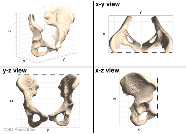
Pre-defined alignment of the pelvis in three planes based on landmark locations. Upper-right: on the x–y view, the anterior superior iliac spines (ASIS) were aligned. Lower-left: on the y–z view, the two iliac crests were aligned at the most superior point. Lower-right: on the x–z view, the ASIS and the pubic tubercle were aligned.
Fig. 2.
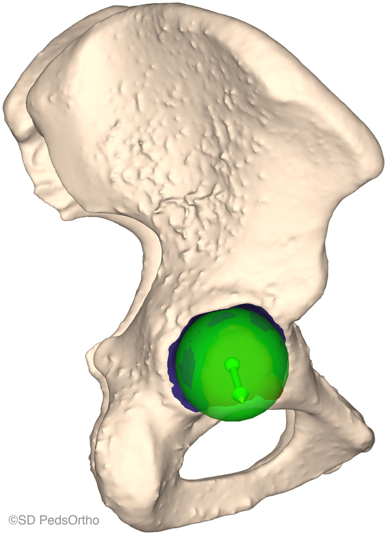
Best-fit sphere calculated using least-square regression superimposed on the acetabulum. The center of the sphere is shown by a green dot and the acetabulum direction vector by an arrow.
Fig. 3.
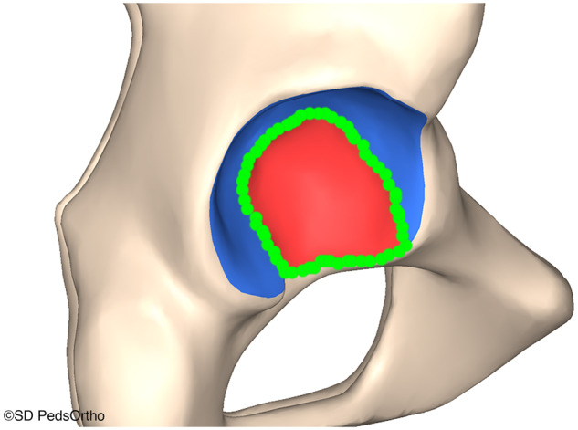
Drawing the cotyloid fossa/articular surface boundaries manually. Green circles indicate a user’s hand drawn tracing.
Fig. 4.
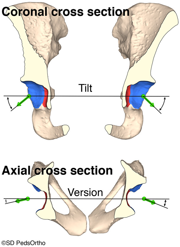
Coronal and axial cross sections of a pelvic model illustrating the technique of measuring tilt, in the coronal plane, and version, in the axial plane.
Fig. 5.

(A) Coronal cross section of the 3D model illustrating coverage angle calculation. The total coverage angle is the angle between the line connecting the center of the best-fit spheres for each pelvis (identified by the two green dots) and the edge of the acetabulum. The coverage angle for the fossa is the line connecting the center of the best-fit spheres and the edge of the fossa (identified as the red area). The weight-bearing coverage area is the difference between the two (WBR/L = weight-bearing right/left and FR/L = Fossa right/left). (B) Diagram of the five clinically pertinent coverage angle octants of the acetabulum. The coverage angle reported for the octant section is the average of the coverage angles within the specified 45° (or octant) of the acetabulum edge.
Normal database
Our institution has performed the analysis, as described above, on a series of patients without a history of hip disease/abnormality. We have compiled a cohort of 162 patients (73 male and 89 female) between the ages of 8 and 19 years who had an abdominal/pelvis CT as part of an emergency department work up. The most common indications for the CT were appendicitis and trauma. The CTs were viewed, and the radiology reports, as well as the patient’s medical history, were screened to ensure that there was no evidence of hip disease prior to undergoing measurement and analysis. 3D reconstructions and pelvic measurements were performed as described in the preceding paragraphs. The results of this dataset have been published in part [16]. This allows for a normal comparison with the surgical candidate and is critical in determining the area(s) of acetabular abnormality.
Additionally, a z-score was used to compare a surgical candidate to an age- and sex-matched normal cohort. The z-score was calculated by subtracting the mean value of the normal subjects from the value of the surgical candidate and then dividing that number by the standard deviation of the mean for the age- and sex-matched normal cohort. This calculation was performed for each section of the acetabulum and a graph was created (Fig. 6). z-Scores over 2 or below −2 are considered abnormal. This identified the areas of over- or under-coverage of the acetabulum and allowed the surgeon to plan his/her procedure accordingly. The total amount of time per pelvis to complete this analysis was ∼60 min.
Fig. 6.

(A) AP radiograph of an 11-year-old female with left acetabular dysplasia. (B) A graphical representation of this child’s z-scores for each section of the acetabulum. If the child’s acetabulum was exactly the same as the mean, the z-scores for each section would be zero. Values over 2 would represent over-coverage of that section; values below −2 indicate under-coverage of that section. This graph indicates that this child has a posteriorly deficient acetabulum.
Statistical analysis
Two observers performed the entire acquisition, reconstruction and analysis procedure outlined above on a set of 10 patients with at least one dysplastic hip as determined by chart review. One observer repeated the entire procedure outlined after 2 months. Intra-class correlation coefficient (ICC) was used to evaluate the reproducibility of the process. ICC was performed using IBM SPSS Statistics (version 25; IBM, Armonk, NY, USA). Significance was defined as P < 0.05. ICC scores ≥0.8 were considered acceptable.
RESULTS
Version, tilt and surface area were found to have excellent reproducibility, all three had an ICC >0.87 for both inter- and intra-observer reliability. The measurements that depend on the accurate identification of the border between the fossa and the weight-bearing surface of the acetabulum were generally found to be poorly reproducible, with ICC values ranging from 0.346 to 0.859 and maximum P values of 0.162. However, when evaluating each octant of the entire acetabulum (as in Fig. 5B, fossa + weight-bearing surface), the process was found to be quite reproducible, with ICC values ranging from 0.805 to 0.943. Reproducibility results for each section measured are shown in Tables I and II.
Table I.
Intra-observer reproducibility
| ICC | 95% CI—lower | 95% CI—upper | Sig., P | |
|---|---|---|---|---|
| Version | 0.997 | 0.987 | 0.999 | <0.001 |
| Tilt | 0.980 | 0.924 | 0.995 | <0.001 |
| Surface area | 0.972 | 0.888 | 0.993 | <0.001 |
| Posterior section—WB | 0.695 | 0.145 | 0.915 | 0.011 |
| Superior–posterior section—WB | 0.498 | −0.073 | 0.841 | 0.048 |
| Superior section—WB | 0.544 | −0.010 | 0.858 | 0.028 |
| Superior–anterior section—WB | 0.346 | −0.371 | 0.789 | 0.162 |
| Anterior section—WB | 0.859 | 0.533 | 0.963 | <0.001 |
| Posterior section—fossa | 0.800 | 0.398 | 0.946 | 0.001 |
| Superior–posterior section—fossa | 0.621 | 0.050 | 0.890 | 0.008 |
| Superior section—fossa | 0.594 | 0.008 | 0.880 | 0.01 |
| Superior–anterior section—fossa | 0.733 | 0.209 | 0.927 | 0.007 |
| Anterior section—fossa | 0.840 | 0.502 | 0.957 | 0.001 |
| Posterior section—total | 0.942 | 0.790 | 0.985 | <0.001 |
| Superior–posterior section—total | 0.934 | 0.767 | 0.983 | <0.001 |
| Superior section—total | 0.879 | 0.608 | 0.968 | <0.001 |
| Superior–anterior section—total | 0.805 | 0.423 | 0.947 | 0.001 |
| Anterior section—total | 0.883 | 0.532 | 0.971 | <0.001 |
ICC, intra-class correlation coefficient; WB, weight bearing.
Table II.
Inter-observer reproducibility
| ICC | 95% CI—lower | 95% CI—upper | Sig., P | |
|---|---|---|---|---|
| Version | 0.990 | 0.957 | 0.998 | <0.001 |
| Tilt | 0.979 | 0.917 | 0.995 | <0.001 |
| Surface area | 0.871 | 0.035 | 0.975 | <0.001 |
| Posterior section—WB | 0.601 | −0.010 | 0.884 | 0.029 |
| Superior–posterior section—WB | 0.421 | −0.134 | 0.805 | 0.073 |
| Superior section—WB | 0.678 | 0.148 | 0.908 | 0.005 |
| Superior–anterior section—WB | 0.532 | −0.156 | 0.862 | 0.056 |
| Anterior section—WB | 0.853 | 0.519 | 0.961 | 0.001 |
| Posterior section—fossa | 0.822 | 0.464 | 0.952 | 0.001 |
| Superior–posterior section—fossa | 0.628 | 0.062 | 0.892 | 0.008 |
| Superior section—fossa | 0.685 | 0.114 | 0.913 | 0.003 |
| Superior–anterior section—fossa | 0.858 | 0.528 | 0.963 | 0.001 |
| Anterior section—fossa | 0.720 | 0.226 | 0.922 | 0.007 |
| Posterior section—total | 0.943 | 0.792 | 0.985 | <0.001 |
| Superior–posterior section—total | 0.930 | 0.755 | 0.982 | <0.001 |
| Superior section—total | 0.897 | 0.653 | 0.973 | <0.001 |
| Superior–anterior section—total | 0.832 | 0.454 | 0.956 | 0.001 |
| Anterior section—total | 0.941 | 0.786 | 0.985 | <0.001 |
ICC, intra-class correlation coefficient; WB, weight bearing.
DISCUSSION
This manuscript presents a unique method to quantify acetabular morphology. Our purpose is to share the detailed technique used to acquire 3D data and report our inter- and intra-rater variability for data acquisition. This is similar to previously reported 3D acetabular coverage analysis of a varied age cohort of 27 normal (15–61 years) and 27 dysplastic (14–41 years) hips with inter-rater variability (2 raters) of 0.96 [17]. The acetabulum is a 3D structure with complex primary and secondary ossification centers making quantification of acetabular abnormalities challenging [18]. Traditional radiographs can be used to measure the slope of the sourcil (weight-bearing region) or the lateral edge of the acetabulum [5–8]; however, it is difficult to quantify the anterior and posterior walls accurately. Previous studies have attempted to measure anterior and posterior wall indices in relation to the femoral head; however, they have been shown to be dependent on pelvic position and radiograph acquisition technique [9–13]. Also, normal dimensions of acetabular shape have been found to be significantly different between sexes and change with growth, making previously published norms difficult to interpret [16].
The current technique gives a clear and reproducible measurement of acetabular morphology that can be directly compared with a cohort of age- and sex-matched typically developing children. This analysis has been used at our institution for past 2 years when treating patients with pediatric hip disease, ranging from dysplasia to over-coverage, as in patients with FAI. It has allowed our surgeons to understand the 3D shape of each individual’s acetabulum, share these findings with patients and their parents to demonstrate the magnitude and location of the clinical abnormality and perform patient-specific surgical corrections to optimize the shape and coverage of the hip.
To demonstrate the clinical application of this technique, we present a 16-year-old female who presented to our clinic with left hip pain. She was treated as an infant for a left dislocated hip and underwent open reduction followed by brace treatment. She was lost to follow-up during childhood and then returned as a teenager with left hip symptoms. This technique was used to quantify acetabular morphology and for surgical planning. The acetabular coverage of this child’s hip was compared using z-scores to an age- and sex-matched cohort of typical hips with no evidence of dysplasia. Based on the relatively retroverted position of the acetabulum, the surgeon determined that this patient should have an anteverting periacetabular osteotomy to obtain improved posterior and lateral coverage. This type of acetabular deformity is less common in patients with typical DDH and 3D appreciation of the specific region of deficiency was critical to appropriately manage this patient’s dysplasia. After surgical correction, a low-dose CT was obtained to demonstrate appropriate correction of the acetabular position (Fig. 7).
Fig. 7.
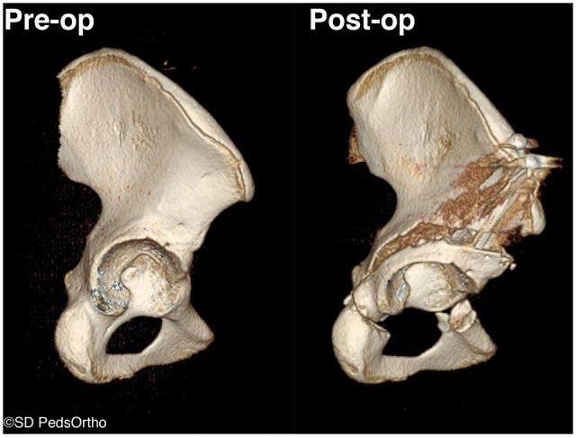
Pre- and post-operative 3DCT reconstructions from the direct lateral view. Pre-operatively, the superior and posterior surfaces of the acetabulum are clearly seen. After corrective osteotomy, you can no longer see the superior surface of the acetabulum and the posterior surface that is visible is similar to the visible surface of the anterior portion of the acetabulum.
Over 2 years of use, we have found some limitations with the technique that requires improvement. For example, manually tracing the fossa boundaries can be challenging, especially with lower resolution CT images. Additionally, for the code to produce accurate measurements, the acetabulum must be ossified enough for the bony morphology to be a reasonable representation of the bony and cartilaginous shape of the acetabulum. For this reason, we do not have a normal cohort for comparison for patients below the age of 8 years. Another limitation is that we are using a comparison group of normal hips that are matched based on chronological age range and not skeletal age. This could be a problem if the comparison sample consists of subjects who consistently have a skeletal age that is different from their chronological age. Finally, each geographical region may need to create their own database of normal hips for comparison with their patient population as variation in acetabular morphology likely exists among geographical regions.
By sharing the code and technique described here, we hope to encourage more centers to begin quantifying acetabular morphology for surgical planning. By increasing the volume of normal and abnormal patients, we aim to refine the technique and improve the precision of detecting patient-specific abnormalities. Future derivations of this technique need to account for the shape and position of the femoral head. This will likely require acquisition of CT torsional profiles to determine the 3D shape of the femur and its relation to the acetabulum. Additionally, we need to be able to accurately measure bony morphology using MR techniques to minimize patient exposure to ionizing radiation.
SUPPLEMENTARY DATA
Supplementary data are available at Journal of Hip Preservation Surgery online.
Supplementary Material
ACKNOWLEDGMENTS
We would like to thank Raghav Badrinath, MD, for completing a set of measurements allowing us to present inter-observer reliability for this measurement technique.
CONFLICT OF INTEREST STATEMENT
J.D.B., H.B., J.D.D. and C.L.F. have nothing to disclose. V.V.U. has the following disclosures unrelated to the submitted work: BroadWater, DePuy, A Johnson & Johnson Company and Nuvasive: paid presenter or speaker. EOS Imaging and nView: research support. Globus Medical: paid consultant. Imagen: stock or stock options. OrthoPediatrics: paid consultant, paid presenter or speaker. Wolters Kluwer Health—Lippincott Williams & Wilkins: publishing royalties, financial or material support.
Contributor Information
Vidyadhar V Upasani, Division of Orthopedics, Rady Children’s Hospital, San Diego 3020 Children’s Way, Mail Code 5062 San Diego, CA 92123, USA; Department of Orthopaedic Surgery, University of California, San Diego 200 W. Arbor Drive, MC 8894 San Diego, CA 92103, USA.
James D Bomar, Division of Orthopedics, Rady Children’s Hospital, San Diego 3020 Children’s Way, Mail Code 5062 San Diego, CA 92123, USA.
Harsha Bandaralage, Division of Orthopedics, Rady Children’s Hospital, San Diego 3020 Children’s Way, Mail Code 5062 San Diego, CA 92123, USA.
Joshua D Doan, Division of Orthopedics, Rady Children’s Hospital, San Diego 3020 Children’s Way, Mail Code 5062 San Diego, CA 92123, USA.
Christine L Farnsworth, Division of Orthopedics, Rady Children’s Hospital, San Diego 3020 Children’s Way, Mail Code 5062 San Diego, CA 92123, USA.
REFERENCES
- 1. Khanna V, Beaulé PE. Defining structural abnormalities of the hip joint at risk of degeneration. J Hip Preserv Surg 2014; 1: 12–20. [DOI] [PMC free article] [PubMed] [Google Scholar]
- 2. Parvaresh KC, Pennock AT, Bomar JD et al. Analysis of acetabular ossification from the triradiate cartilage and secondary centers. J Pediatr Orthop 2018; 38: e145–50. [DOI] [PubMed] [Google Scholar]
- 3. Albers CE, Rogers P, Wambeek N et al. Preoperative planning for redirective, periacetabular osteotomies. J Hip Preserv Surg 2017; 4: 276–88. [DOI] [PMC free article] [PubMed] [Google Scholar]
- 4. Chadayammuri V, Garabekyan T, Jesse M-K et al. Measurement of lateral acetabular coverage: a comparison between CT and plain radiography. J Hip Preserv Surg 2015; 2: 392–400. [DOI] [PMC free article] [PubMed] [Google Scholar]
- 5. Tönnis D. Congenital Dysplasia and Dislocation of the Hip in Children and Adults. Berlin, Heidelberg: Springer-Verlag, 1987. [Google Scholar]
- 6. Wiberg G. Shelf operation in congenital dysplasia of the acetabulum and in subluxation and dislocation of the hip. J Bone Joint Surg Am 1953; 35-A: 65–80. [PubMed] [Google Scholar]
- 7. Sharp IK. Acetabular dysplasia: the acetabular angle. J Bone Joint Surg Br Vol 1961; 43-B: 268–72. [Google Scholar]
- 8. Mittal A, Bomar JD, Jeffords ME et al. Defining the lateral edge of the femoroacetabular articulation: correlation analysis between radiographs and computed tomography. J Child Orthop 2016; 10: 365–70. [DOI] [PMC free article] [PubMed] [Google Scholar]
- 9. Monazzam S, Bomar JD, Agashe M, Hosalkar HS. Does femoral rotation influence anteroposterior alpha angle, lateral center-edge angle, and medial proximal femoral angle? A pilot study. Clin Orthop Relat Res 2013; 471: 1639–45. [DOI] [PMC free article] [PubMed] [Google Scholar]
- 10. Tannast M, Hanke MS, Zheng G et al. What are the radiographic reference values for acetabular under- and overcoverage? Clin Orthop Relat Res 2015; 473: 1234–46. [DOI] [PMC free article] [PubMed] [Google Scholar]
- 11. Tannast M, Fritsch S, Zheng G et al. Which radiographic hip parameters do not have to be corrected for pelvic rotation and tilt? Clin Orthop Relat Res 2015; 473: 1255–66. [DOI] [PMC free article] [PubMed] [Google Scholar]
- 12. Ross JR, Nepple JJ, Philippon MJ et al. Effect of changes in pelvic tilt on range of motion to impingement and radiographic parameters of acetabular morphologic characteristics. Am J Sports Med 2014; 42: 2402–9. [DOI] [PubMed] [Google Scholar]
- 13. Jackson TJ, Estess AA, Adamson GJ. Supine and standing AP pelvis radiographs in the evaluation of pincer femoroacetabular impingement. Clin Orthop Relat Res 2016; 474: 1692–6. [DOI] [PMC free article] [PubMed] [Google Scholar]
- 14. Bockhorn L, Gardner SS, Dong D et al. Application of three-dimensional printing for pre-operative planning in hip preservation surgery. J Hip Preserv Surg 2019; 6: 164–9. [DOI] [PMC free article] [PubMed] [Google Scholar]
- 15. Murray DW. The definition and measurement of acetabular orientation. J Bone Joint Surg Br 1993; 75-B: 228–32. [DOI] [PubMed] [Google Scholar]
- 16. Peterson JB, Doan J, Bomar JD, Wenger DR et al. Sex differences in cartilage topography and orientation of the developing acetabulum: implications for hip preservation surgery. Clin Orthop Relat Res 2015; 473: 2489–94. [DOI] [PMC free article] [PubMed] [Google Scholar]
- 17. Dandachli W, Kannan V, Richards R et al. Analysis of cover of the femoral head in normal and dysplastic hips: new CT-based technique. J Bone Joint Surg Br 2008; 90-B: 1428–34. [DOI] [PubMed] [Google Scholar]
- 18. Acuña AJ, Samuel LT, Mahmood B, Kamath AF. Systematic review of pre-operative planning modalities for correction of acetabular dysplasia. J Hip Preserv Surg 2019; 6: 316–25. [DOI] [PMC free article] [PubMed] [Google Scholar]
Associated Data
This section collects any data citations, data availability statements, or supplementary materials included in this article.