Dynamic network connectivity predicts subjective cognitive decline: the Sino-Longitudinal Cognitive impairment and dementia study

Abstract

Subjective cognitive decline (SCD) is the preclinical stage of Alzheimer’s disease (AD), the most common neurodegenerative disease in the elderly. We collected resting-state functional MRI data and applied novel graph-theoretical analyses to investigate the dynamic spatiotemporal cerebral connectivities in 63 individuals with SCD and 67 normal controls (NC). Temporal flexibility and spatiotemporal diversity were mapped to reflect dynamic time-varying functional interactions among the brain regions within and outside communities. Temporal flexibility indicates how frequently a brain region interacts with regions of other communities across time; spatiotemporal diversity describes how evenly a brain region interacts with regions belonging to other communities. SCD and NC differed in large-scale brain dynamics characterized by the two measures, which, with support vector machine, demonstrated higher classification accuracies than conventional static parameters and structural metrics. The findings characterize dynamic network dysfunction that may serve as a biomarker of the preclinical stage of AD.

Introduction

As the main cause of dementia, Alzheimer’s disease (AD) is one of the greatest health-care challenges of the twenty-first century (Scheltens et al. 2016). In the US more people died of AD than of breast cancer and prostate cancer combined (Patterson 2018). More than 100 drugs have been tested in the treatment of AD since 1998, but only four have been approved by the FDA and the efficacy of these medications appeared to be limited (Patterson 2018). Current effort in medication development is directed at the earlier stage when memory loss is mild or absent in patients with the hallmarks of AD pathology (McDade and Bateman 2017). Subjective cognitive decline (SCD) refers to individuals’ perceived persistent memory decline relative to their previous level of performance and self-concerns about the cognitive decline. Individuals with SCD show an increased likelihood of demonstrating bio-markers consistent with AD and risk for future cognitive decline and dementia (Jessen et al. 2014). SCD represents the earliest symptomatic manifestation of AD, earlier than the prodromal stage or mild cognitive impairment (MCI) (Rabin et al. 2017; Sperling et al. 2011; Jessen et al. 2014). Therefore, research of the neural processes underlying SCD is critical to our understanding of the etiology and may facilitate the development of new and effective treatment of AD.

The human brain is an interacting, dynamic system supported by the intrinsic architecture of large-scale functional coupling among brain regions that varies across time (Power et al. 2011; Bressler and Menon 2010; Liu et al. 2018). A promising non-invasive technique to identify spontaneous activities in vivo, resting-state functional magnetic resonance imaging (rs-fMRI) helps to detect the intrinsic cerebral functional organization under normal and pathological conditions (Gusnard et al. 2001; Zhang and Raichle 2010). As with amnestic MCI (aMCI) and AD dementia patients, individuals with SCD exhibited disruptions in brain structural connectome and in functional integration and segregation (Shu et al. 2018; Shu et al. 2012; Viviano et al. 2018), suggesting the importance of identifying network connectivity changes in this early state of AD.

The great majority of imaging studies have employed time-averaged analytical approaches to examine the static organization of brain networks, under the assumption that functional connectivity over the data collection period is relatively static for the limited temporal resolution of fMRI (Calhoun et al. 2014; Hutchison et al. 2013; Chen et al. 2016a; Zalesky et al. 2014). However, cerebral functional connectivity may not be truly static considering physiological noise, scanner drift, and fluctuation of subjects’ attention (Morgan et al. 2015). Further, human cognition is reported to be influenced by unknown, latent mental processes that can change with time (Taghia et al. 2018) and interact dynamically over time (Kim et al. 2017; Menon and Uddin 2010). Evidence has accumulated to suggest the importance in considering the temporal features of blood oxygenation level-dependent (BOLD) signals in order to fully explore brain functions (Hutchison et al. 2013).

The coordination of neural population activities is dynamic and context dependent. Brain dynamics vary in network properties over time, balancing efficient information processing and metabolic requirements (Zalesky et al. 2014), to support cognition (Allen et al. 2014; Calhoun et al. 2014; Chang and Glover 2010; Kang et al. 2011; Thompson et al. 2013). Dynamic functional connectivity quantifies network changes over time, and may capture the neural processes critical to the etiology of neurodegenerative diseases (Damaraju et al. 2014; Kaiser et al. 2016; de Lacy et al. 2017; Yaesoubi et al. 2017). A few studies showed that AD was associated with increased variability in dynamic properties of brain activity and connectivity (Jie et al. 2018; Cordova-Palomera et al. 2017; Brenner et al. 2018). Compared to MCI and SCD, individuals with AD dementia presented alterations in both static (mainly in putamen, dorsal parietal and default-mode regions) and dynamic (mainly among temporal, frontal-superior and default-mode regions) functional connectivity, along with decreases in global metastability (Cordova-Palomera et al. 2017). Jie et al. constructed the dynamic connectivity network by using non-overlapping time window approach and integrated both temporal and spatial properties of networks to distinguish MCI from NC. The authors found that cognitive dysfunction in early MCI might be associated with disrupted functional configurations in the posterior cingulate gyrus, hippo-campus, amygdala, precuneus and temporal lobe, in keeping with previous studies (Jie et al. 2018). Moreover, aMCI was associated with the loss of neural network dynamics in posterior components of the default mode network, which were related to reduced flexibility in resource allocation (Brenner et al. 2018). These findings together suggested the vulnerability of network dynamics in AD.

Graphic theoretical metrics have become increasingly popular in mapping dynamic network connectivity and detecting topological functional abnormality (Zhang et al. 2018; Chen et al. 2016a). In dynamic graph theoretic analyses, the time series is divided into multiple, smaller time segments with a sliding window. As such, the analyses capture the dynamic functional changes of the brain, which would not be possible with the conventional approaches that involved averaged data time points. As a stable feature of the dynamic patterns of time-varying connectivity (Chen et al. 2016a), temporal flexibility quantifies how frequently a brain region interacts with regions outside its own community over time. High temporal flexibility implies that the region mainly interacts with regions belonging to other communities. Spatiotemporal diversity quantifies how uniformly a brain region interacts with regions of other communities across time. High spatiotemporal diversity suggests that these interactions are evenly distributed across communities (Zhang et al. 2018; Chen et al. 2016a). A brain region with high temporal flexibility may not demonstrate high spatiotemporal diversity if they mainly interact with regions in only one community. Spatiotemporal diversity provides complementary information about the spatial distribution of time-varying connectivity (Zhang et al. 2018; Chen et al. 2016a). Together, spatiotemporal diversity and temporal flexibility provide critical metrics of functional brain dynamics (Chen et al. 2016a).

The current study aimed to identify changes in cerebral spatiotemporal dynamic properties in individuals with SCD, as compared to NC, in order to inform the neuropathological processes during early stages of AD. We examined spatiotemporal diversity and temporal flexibility of the whole brain, and employed a support vector machine (SVM) to investigate the group classification accuracy of these features in comparison with conventional static graphic and morphometric features. We posited that dynamic functional connectivity would already be altered in SCD. Further, dynamic functional connectivity would provide more specific neural features, as compared to conventional static functional measures, in distinguishing SCD from normal aging. Finally, dynamic patterns of regional connectivities would correlate with cognitive performance (neuropsychological test scores) in SCD.

Materials and methods

Participants

A total of 150 right-handed Chinese participants (75 SCD and 75 NC) were enrolled from the Xuanwu Hospital, Capital Medical University, as part of the Sino-Longitudinal Cognitive Impairment and Dementia Study (SILCODE), from March 20th, 2017 to April 17th, 2018. The SILCODE is a prospective cohort study of patients with SCD, MCI, AD dementia. Participants are enrolled from the memory clinic and community and from referrals by primary care physicians. The present study was registered on ClinicalTrials.gov (Identifier: NCT03370744). The protocol was approved by the institutional review board of Xuanwu Hospital of Capital Medical University, and all participants completed a written informed consent prior to the study.

As proposed by the SCD Initiative (Jessen et al. 2014), the inclusion criteria of SCD were as follows: (1) self-perceived continuous decline in memory that is unrelated to an acute event such as relative’s death and loss of job; (2) self-concerns or worries about memory decline; and (3) performance on standardized neuropsychological tests within the normal range as adjusted by age, gender, and education. The criteria for NC were: (1) no self-report of decline in memory or having memory complaints but without concerns; (2) normal performance on the standard neuropsychological tests.

Exclusion criteria for SCD and NC included: (1) MCI, dementia, or any other neurological conditions that may cause memory complaints (i.e., Parkinson’s disease, epilepsy, or encephalitis); (2) history of stroke; (3) major psychiatric disorders affecting cognition, such as depression with Hamilton Depression Scale (HAMD) > 24; (4) systemic diseases that could cause cognitive impairments (e.g., syphilis, thyroid dysfunctions, severe anemia, or HIV); (5) alcohol or substance abuse or dependence; (6) severe vision or hearing impairment; (7) inability to complete neuropsychological tests; and (8) contraindications for MRI.

Clinical and neuropsychological assessments

All subjects underwent a standard clinical evaluation that included medical and family history, current medications, physical examination, and routine blood tests; assessment with a battery of neuropsychological tests; and structural MRI scans.

The neuropsychological battery included tests of episodic memory (Auditory Verbal Learning Test – HuaShan version [AVLT-H]) (Zhao et al. 2015), language (Animal Fluency Test [AFT], 30-item Boston Naming Test [BNT]), executive function (Shape Trails Test Parts A and B [STT-A, STT-B]) (Zhao et al. 2013), general cognitive ability (Chinese version of Mini Mental State Examination [MMSE], Montreal Cognitive Assessment-basic [MoCA-B] (Chen et al. 2016b), and memory and executive function screening instrument [MES] (Guo et al. 2012)). Subjects were also evaluated with the Functional Activities Questionnaire (FAQ) (Pfeffer et al. 1982), 15-item short form of the Geriatric Depression Scale (GDS) (Yesavage et al. 1982), Hamilton Anxiety Scale (HAMA) (Hamilton 1959), HAMD (Hamilton 1960), and the Neuropsychiatric Inventory (NPI) (Cummings 1997). Cognitive testing was performed by trained neuropsychologists.

APOE genotyping

APOE ε4 is a major genetic risk factor for AD (Scheltens et al. 2016). The risk for AD is more than 50% for APOE ε4 homozygotes and 20–30% for APOE ε3 and APOE ε4 heterozygotes, as compared to an overall risk of 11% for men and 14% for women irrespective of the APOE genotype (Genin et al. 2011). Therefore, we collected the blood and extract serum to test the APOE genotyping. The DNA for each subject was extracted for SNPs rs7412 and rs429358 forming the APOE ε2/ε3/ε4 haplotype. The standard Sanger sequencing method (Sangon, Shanghai, China) was used for the genotyping of APOE with following primers: 5′-ACGCGGGCACGGCTGTCCAAGG-3′ (forward) and 5′-GGCGCTCGCGGATGGCGCTGA-3′ (reverse). The following conditions were used to amplify the APOE: 1 cycle of 98 °C for 10 s, 35 cycles of 72 °C for 5 s, 1 cycle of 72 °C for 5 min. PCR was performed in a final volume of 30 μl, containing 10 pmol of forward and reverse primers and 50 ng of genomic DNA template, using PrimeSTAR HS DNA Polymerase with GC Buffer (Takara Bio).

Imaging parameters

All participants were scanned on an integrated simultaneous 3.0 Tesla TOF PET/MR (SIGNA PET/MR, GE Healthcare, Milwaukee, WI, USA) at the Xuanwu Hospital of Capital Medical University. The rs-fMRI scan lasted 8 min. 3D BRAVO T1-weighted sagittal images were obtained using the following parameters: SPGR sequence, repetition time (TR) = 6.9 ms, echo time (TE) = 2.98 ms, flip angle (FA) = 12°, inversion time (TI) = 450 ms, field of view (FOV) = 256 × 256 mm², matrix = 256 × 256, gap = 0, slice thickness = 1 mm, slice number = 192, and voxel size = 1 × 1 × 1 mm³. Single-shot gradient-echo EPI sequence, TR = 2000 ms, TE = 30 ms, FA = 90°, FOV = 224 × 224 mm², data matrix = 64 × 64, gap = 1.0 mm, slice thickness = 4.0 mm, slice number = 28, slice order = interleaved, and voxel size = 3.5 × 3.5 × 4 mm³. MR images were inspected by an experienced neuro-radiologist for quality and incidental findings.

Imaging data pre-processing

All data were first analyzed with Data Processing & Analysis for (Resting-State) Brain Imaging (DPABI, Key Laboratory of Behavioral Science and Magnetic Resonance Imaging Research Center, Chinese Academy of Sciences, China. http://www.rfmri.org/dpabi) (Yan et al. 2016). In the preprocessing of BOLD data, the first 5 frames of BOLD data were discarded to ensure that only signals during steady-state equilibrium between radio frequency pulsing and relaxation were included in analyses. Images of each participant were realigned with 12 realignment parameters (use 3 translations, 3 rotations, and their first temporal derivatives) and corrected for slice timing. These images were co-registered with the structural image and then segmented for normalization to a Montreal Neurological Institute EPI template (Ashburner and Friston 1999; Friston et al. 1995). A band-pass filter (0. 001 Hz < f < 0.01 Hz) was applied to remove low-frequency signal drifts and increase the signal noise ratio. Images were smoothed with a Gaussian kernel of 4 mm at full width at half maximum. Finally, all data were detrended.

Feature extraction

Brain template

We used a functional brain template which contains 268 brain regions (Finn et al. 2015). These brain regions were divided into 8 functional networks.

Dynamic graph theoretic features

The processing flow for dynamic graph theoretic features is shown in Fig. 1 (Chen et al. 2016a). The time series of each brain region were averaged across voxels, and the average time series of each brain region defined the node for time varying functional connectivity analysis.

Fig. 1.

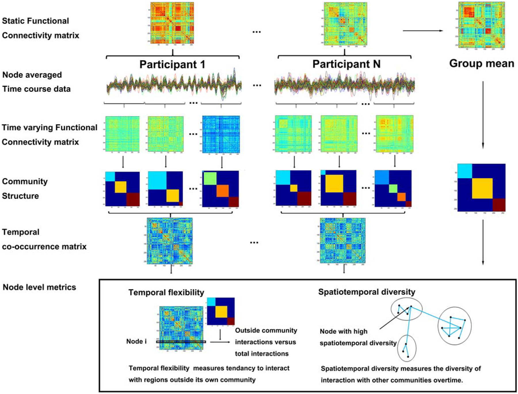
The computation of dynamic graph theoretic parameters. A sliding window approach was used to quantify the time-varying changes in the community structure of intrinsic functional connectivity. The temporal co-occurrence matrix was based on the Louvain community detection algorithm. The temporal flexibility and spatiotemporal diversity were computed by an optimized community detection algorithm

To obtain dynamic functional connectivity between nodes, a sliding window with no overlap between windows was applied to the time series. Exponentially decaying weights were applied to each time point within a window (Zalesky et al. 2014). The exponentially decaying weights were computed as:

$$W_t=W_0{e}^{(t-T){/}_{\theta }},t=1,\cdots ,T$$

where $W_0=\frac{1-e^{-{/}_{\theta }^1}}{1-e^{-{/}_{\theta }^T}}$ is the t^th time point within the sliding window; T is the window length (20 TRs = 40s); and the exponent θ controls the influence from distant time points, set to a third of the window length. With the weighted Pearson correlation between the time-series of any two nodes x_t and y_t, we computed the connectivity matrix for each time window.

$${\text{r}}_w=\frac{{\sum }_{t=1}^T{w}_t\left(x_t-\overline{x}\right)\left(y_t-\overline{y}\right)}{\sqrt{{\sum }_{t=1}^T{w}_t{\left(x_t-\overline{x}\right)}^2}\sqrt{{\sum }_{t=1}^T{w}_t{\left(y_t-\overline{y}\right)}^2}}$$

where $\overline{y}=\frac{{\sum }_{t=1}^T{W}_t{X}_t}{T}$ and $\overline{x}=\frac{{\sum }_{t=1}^T{W}_t{X}_t}{T}$, and the resulting Pearson correlation matrix for each window was z-transformed within the subject for subsequent analysis.

Modularity was used to determine the optimal community structure within the unthresholded connectivity matrix by grouping nodes into non-overlapping communities or modules that maximize intra-modular connectivity and minimize inter-modular connectivity (Newman 2004). Louvain community detection algorithm from the Brain Connectivity Toolbox was employed to identify community structure in both static and time-varying connectivity matrices (Rubinov and Sporns 2010). This algorithm is one of the most widely used modularity optimization algorithms (Blondel et al. 2008). The algorithm optimizes a quality function Q, defined as the difference between the observed intra-modular and inter-modular connectivity, while penalizing assignment of nodes with negative correlations to the same community. The algorithm was repeated 100 times and the results with the highest Q was extracted as the optimal community structure, to compute group static matrix and each subject’s temporal co-occurrence matrix.

To quantify the dynamic connections between different nodes, we computed the temporal co-occurrence matrix based on subject’s optimal community structure as obtained from the Louvain algorithm. The community structure within each sliding window was used to construct an adjacency matrix A_ijtk. When the brain region i and j in the same time window of the subject k was in the same module, the A_ijtk = 1; otherwise A_ijtk = 0. Thus, each time window is a 0–1 matrix, and the temporal co-occurrence matrix C_ijk is temporal average of these 0–1 matrices, with ${\text{C}}_{\text{ijk}}=\frac{{\sum }_{t=1}^T{A}_{\mathit{\text{ijtk}}}}{T}$ (Braun et al. 2015; Mattar et al. 2015; Bassett et al. 2015). It quantifies the proportion of times that the two nodes belonging to the same module, with a higher value indicating a higher frequency that the two nodes belong to the same module.

For each individual, the static connectivity between nodes was computed by applying Pearson correlations on the nodes’ time-series. The resulting correlation matrices from individual subjects were z-transformed and averaged to form a group averaged connectivity matrix each for SCD and NC. Modularity analysis was based on group averaged connectivity matrix by Louvain algorithm, repeated 100 times to determine the optimal static community structure for the computation of node-level metrics.

We defined the dynamic graph theoretic features of each node – temporal flexibility and spatiotemporal diversity – with the temporal co-occurrence matrix C_ijk and the group static community as defined earlier.

The temporal flexibility of node i and subject k was computed as

$$f_{ik}=\frac{{\sum }_{j\notin u_i}{c}_{ijk}}{{\sum }_{j\ne i}{c}_{ijk}}$$

where C_ijk is the temporal co-occurrence matrix for subject k, u_i is the community to which node i belongs, and ∑_j∉uic_ijk measures the total frequency with which node i interacts with nodes outside its native community (Mucha et al. 2010). Temporal flexibility of the node denotes the tendency of deviation from its own native community and interaction with nodes from other community.

The spatiotemporal diversity of node i and subject k was computed as:

$$h_{ik}=-\frac{{\sum }_{u\in M}{p}_{ik}(u){\text{log}}_{p_{ik}}(u)}{\text{log}(m)}$$

where $p_{ik}(u)=\frac{s_{ik}(u)}{s_{ik}}$, s_ik is the degree of node i among all communities for subject k, s_ik(u) is the degree of node i in community u for subject k, m is the total number of communities, and M is the set of communities (Fornito et al. 2012). Nodes with high spatiotemporal diversity scores are those with relatively spatially varied distribution of time-varying interactions with all communities and are putative loci for information integration between communities.

Static graph theoretic features

We analyzed static graph theoretic features using the toolbox GRETNA (http://rfmri.org/taxonomy/term/118) (Wang et al. 2015). The BOLD time series of each subject were divided and averaged for each brain region (template). The Pearson correlation coefficient between brain regions was calculated pair-wise to build the functional correlation matrix as inputs for GRETNA. The static graph theoretic parameters such as the degree centrality, betweenness centrality, nodal efficiency, nodal local efficiency, rich-club analysis and participant coefficient of each brain region of each subject were also computed based on the correlation matrix. The degree centrality for a given brain region reflects its information communication capacity in the functional network. The betweenness centrality for a given brain region characterizes its effect on information flow between other brain regions. The nodal efficiency characterizes the efficiency of parallel information transfer of a brain region in the network. The nodal local efficiency for a given brain region measures how efficient the communication is among the first neighbors of this brain region when it is removed from the network. The rich-club architecture indicates that the hub brain regions are more densely connected among themselves than non-hub brain regions and thus form a highly interconnected club. The rich-club architecture reflects the modularity efficiency of the whole brain. Here, with 34 brain regions to be the rich-club (see Results), the rich-club features were not sparse. The participant coefficient reflects the ability of an index node in maintaining communication between its own module and the other modules. The module was defined by the static group modularity with greedy optimization algorithm with all subjects’ mean functional correlation matrix in the GRETNA.

The sign of matrix in network configuration is absolute. The network sparsity was utilized to select the threshold from 0.01 to 0.5, with 0.01 step-length. The ‘Network Type’ of ‘Network Configuration’ was set to ‘Weight’ according to the inputs. We obtained 50 different static graph theoretic parameters under different thresholds, and employed the threshold 0.02. The ratio of the global efficiency at each threshold in the static graph theoretic parameters and the corresponding threshold was maximum, indicating that the chosen network had the fewest number of edges and highest global efficiency, eliminating the effects of network sparsity. We used the static graph theoretic parameters as computed by GRETNA to construct static graph theoretic features for SVM.

Structural features

We used voxel-based morphometry analysis to compute gray matter volume (GMV). GMV was estimated based on the pre-treatment process of DPABI (Yan et al. 2016), which included the following steps: building brain template with the raw data; registration of the structural data to the brain template; segmenting the whole brain into gray matter, white matter and cerebrospinal fluid. We obtained the GMV of the whole brain. The affine transformation information was restored, and the GMV of each brain region of each subject was obtained. The GMVof each brain region of every subject was used to construct structural features for SVM. We also computed the total intracranial volume (TIV) and the ratio of GMV to TIV to examine whether it was significantly different between groups.

Classification with support vector machine (SVM)

We used the toolbox of libsvm (https://www.csie.ntu.edu.tw/~cjlin/libsvm/) in MATLAB to construct a binary classification of SCD and NC based on SVM (Chang and Lin 2011). The classification matrix of features was constructed by using all the dynamic graph theoretic parameters, static graph theoretic parameters and gray matter volume, respectively.

In the preprocessing, we divided the whole brain into 268 regions, so the feature dimension of the classification matrix is 268, which was much larger than the 130 subjects in our study. In order to avoid over-fitting, the Lasso sparse algorithm based on least squares estimation was used to reduce the dimension of the feature matrix.

Sparse feature matrix was used to build SVM classifiers. To obtain the most efficient classifier, we adjusted the penalty term parameters of the Lasso sparse formula. Ten-fold cross-classification was performed for ten times. Sparse feature data were divided into 10 parts each time, with nine parts randomly chosen as the training set to build the SVM classifier with a linear kernel and the parameter C is 0.1 (the classification accuracy is highest at this value) and the remaining one part serving as the testing set to obtain classification accuracies (Fig. 2). Each penalty term parameter of the Lasso sparse formula was computed 100 times, and the one that yielded the highest classification accuracy was considered as optimal. The classification accuracy of the most efficient classifier was obtained for further analysis. By changing different feature matrix as the input for SVM, we examined the classification accuracy of different model features.

Fig. 2.

Algorithms for group classification. We used parameters of dynamic graph theory, static graph theory and gray matter volume as the features of SVM classifier, respectively. The Lasso sparse formula was used for feature selection. Ten-fold cross validation was used to obtain the accuracy of the classifier. We adjusted the penalty term parameters of the Lasso sparse formula based on the accuracy to obtain the optimal classification accuracy for each feature

During each cross-classification, the feature dimension was reduced from 268 to 0 by adjusting the penalty term parameters of the Lasso sparse formula. Each parameter adjustment resulted in a classification accuracy rate and retained feature dimension. The highest and mean classification accuracy, and the corresponding mean feature dimension were obtained for each cross-classification and for 10-fold cross-classifications for 10 times were obtained.

We used the receiver operating characteristic (ROC) analysis to examine the “diagnostic” accuracy of a binary classifier system as its discrimination threshold was systematically varied. The area under the ROC curve (AUC) value is equivalent to the probability that a randomly chosen positive example is ranked higher than a randomly chosen negative example. We computed the AUC values for different classifiers based on different classification features, including dynamic and static graph theoretic parameters and GMV.

Brain regions with changes in dynamic graph theoretic parameters

To quantify the contribution of each brain region to the classification of SCD and NC, we analyzed the 100 sets of results with the highest classification accuracy of each dynamic graph theoretic parameter; examined the weight of each brain region as assigned by the lasso sparse algorithm; and examined whether each brain region participated in the classifier.

The average weight and the total number of times at which each brain region participated in the classifier with the highest classification accuracy were also obtained. According to the characteristics of matrix sparseness, the larger the average weight value given by the lasso sparse algorithm, the greater the feature contributes to the classification. The more frequently the feature participates in a classifier, the more stable the feature is with respect to the classification (the maximum number of times of participation is 100, which indicates that the brain region always contributes to the classification during the ten times of ten-fold computation). The top 10 brain regions with the largest and most stable contribution to the classification were selected and compared between SCD and NC in spatiotemporal diversity and temporal flexibility.

Statistical analysis

Chi-square test was used to examine group differences in gender and APOE genotypes, and two sample t test was performed for group difference in age, years of education, and other continuous, behavioral parameters.

For the top 10 brain regions with highest and most stable contribution to the classification, one-way analysis of covariance (ANOVA) was used to examine group differences in dynamic graph theoretic features.

Pearson regressions were performed to examine correlations between dynamic graph theoretic and behavioral parameters for all selected brain regions, with age, gender, years of education, GMV, HAMA, and HAMD scores as covariates, and the results were evaluated with P < 0.05, corrected for false discovery rate (FDR).

Results

Demographic and clinical data

The demographic and clinical information as well as neuropsychological test scores are summarized in Table 1. There was no group difference in age, gender composition, years of education, and APOE-ε4 carrying rate between SCD and NC. HAMD and HAMA scores were significantly higher in SCD than NC; and MoCA-B scores were significantly lower in SCD than NC. There was no significant difference in the ratio of GMV to the TIV. There were no significant differences in other behavioral parameters, including MMSE, AVLT-immediate recall (AVLT-I), AVLT-delayed recall (AVLT-D), AVLT-recognition recall (AVLT-R), STT-A, STT-B, AFT, or BNT scores.

Table 1.

Demographics, neuropsychological test scores and other clinical measures

Variable	SCD N = 63	NC N = 67	P	For λ2
Age(year)	65.8(5.0)	65.3(5.1)	0.355	0.929
Education(year)	11.9(2.8)	11.8(3.1)	0.901	0.125
Gender(F/M)	20/43	28/39	0.236	λ2 = 1.407
HAMD	5.9(4.3)	4.2(4.0)	0.0001	5.504
HAMA	6.3(4.4)	4.4(4.0)	0.0001	5.887
MMSE	28.8(1.2)	28.8(1.2)	0.869	0.165
AVLT-I	6.6(1.2)	6.6(1.5)	0.553	−0.595
AVLT-D	6.7(2.1)	6.9(2.11)	0.443	−0.770
AVLT-R	22.0(1.7)	22.3(1.7)	0.065	−1.867
STT-A	64.2(19.8)	63.9(20.2)	0.874	0.158
STT-B	141.3(35.9)	139.5(33.8)	0.541	0.613
AFT	18.1(4.2)	18.7(4.3)	0.126	−1.541
BNT	24.9(2.4)	25.2(2.8)	0.269	−1.110
MoCA-B	25.3(2.4)	25.7(2.3)	0.028	−2.229
GMV(liter)	0.57(0.50)	0.60(0.06)	0.008	7.243
Gary matter/whole brain ratio	43.1(3.0)%	43.4(2.9)%	0.572	0.321
APOEε4 (±)	18/45	12/55	0.149	λ2 = 2.079

We used chi-square test to compare group differences in gender and APOE genotype, and performed two-sample t test to compare group differences in age, years of schooling, and other continuous, clinical measures, which symbol bold means P< 0.05

Abbreviation: SCD subjective cognitive decline, NC normal controls, HAMD the Hamilton Depression Scale, HAMA the Hamilton Anxiety Scale, MMSE (Chinese version) Mini Mental State Examination, AVLT-I immediate recall of the Auditory Verbal Learning Test, AVLT-D delayed recall of the AVLT, AVLT-R recognition of the AVLT, STT-A Shape Trails Test Parts A, STT-B Shape Trails Test Parts B, AFT the Animal Fluency Test, BNT the 30-item Boston Naming Test, MoCA-B the Montreal Cognitive Assessment-basic, GMV gray matter volume

Classification accuracy of the SVM

We computed the accuracy of SVM classifier with input comprising dynamic graph theoretic features, static graph theoretic features and gray matter volume features. The results are summarized in Table 2.

Table 2.

Classification accuracy and area under the curve (AUC) of brain features

Feature	Highest classification accuracy	Dimension of Highest classification accuracy	Mean classification accuracy	AUC
Spatiotemporal diversity	86.0 ± 2.6%	44	75.4 ± 10.6%	93.2 ± 7.3%
Temporal flexibility	95.0 ±2.1%	26	87.0 ± 7.3%	98.6 ± 2.9%
Degree Centrality	54.3 ± 2.8%	106	49.2 ± 2.4%	54.4 ± 1.7%
Betweenness Centrality	55.9 ± 2.6%	15	51.2 ±4.1%	56.9 ± 1.8%
Nodal efficiency	48.2 ± 2.0%	25	44.5 ± 4.4%	47.3 ± 15.7%
Nodal local efficiency	56.5 ± 2.1%	94	47.2 ± 6.1%	57.9 ± 18.3%
Rich club	53.9 ± 15.8%	34	49.2 ± 12.5%	50.86 ± 18.3%
Participant coefficient	55.5 ± 2.8%	58	49.2 ± 6.0%	55.78 ± 18.2%
Gray matter volume	67.3 ± 3.7%	127	59.0 ±5.1%	72.7 ± 1.4%

The two dynamic graph theoretic features – temporal flexibility and spatiotemporal diversity – distinguished SCD from NC with a mean classification accuracy of 87.0 ± 7.3% and 75.4 ± 10.6%, respectively, both better than conventional static graph theoretic features (44.5 ± 4.4% - 51.2 ± 4.1%) and gray matter volume feature (59.0 ± 5.1%). The superiority of the dynamic graph features was also confirmed with receiver operating characteristic (ROC) analyses (Fig. 3; Table 2).

Fig. 3.

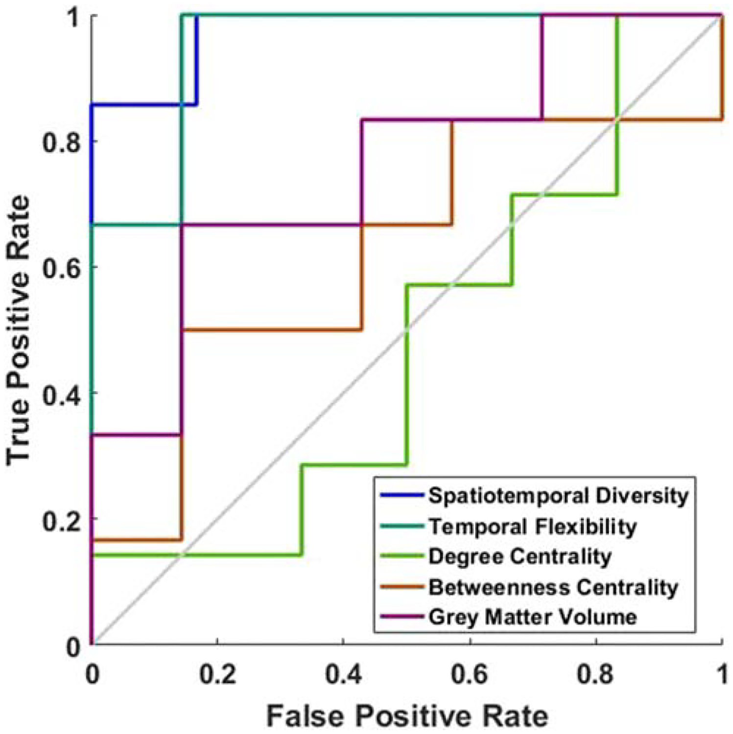
The receiver operating characteristic (ROC) curves of neural features. The two dynamic connectivity measures showed the highest prediction accuracy

Dynamic graph theoretic analysis

The top 10 brain regions with the largest absolute weight value and stable occurrence with respect to the two dynamic graph theoretic features are shown in Table 3. Brain regions were labeled according to the Automated Anatomical Labeling (AAL) atlas.

Table 3.

Top 10 regions with the largest weight of dynamic graph theoretic features

Dynamic feature	Num.	Mean weight	frequency	Brain region (AAL)	Brain region
Spatiotemporal diversity	1	−0.1842	100	Cuneus_R	R Cuneus
	2	0.1711	100	Cerebelum_4_5_R	R Cerebellum
	3	−0.1355	100	Precentral_L	L Precental gyrus
	4	−0.1078	100	Occipital_Mid_R	R Middle occipital gyrus
	5	0.1020	100	Insula_L	L Insula
	6	0.0918	100	Putamen_R	R Lenticular nucleus
	7	−0.0866	98	Calcarine_L	L Calcarine fissure and surrounding cortex
	8	0.0692	97	Thalamus_L	L Thalamus
	9	0.0649	97	Temporal_Inf_R	R Inferior temporal gyrus
	10	−0.0645	96	Parietal_Inf_L	L Inferior parietal
Temporal flexibility	1	0.1229	100	Cerebelum_8_R	R Cerebellum
	2	0.1185	100	Temporal_Inf_L	L Inferior temporal gyrus
	3	−0.0901	100	Postcentral_L	L Postcentral gyrus
	4	−0.0663	99	Parietal_Sup_L	L Superior parietal gyrus
	5	−0.0534	92	Occipital_Inf_L	L Inferior occipital gyrus
	6	−0.0458	97	Frontal_Inf_Orb_L	L Inferior frontal gyrus
	7	−0.0394	89	Fusiform_R	R Fusiform gyrus
	8	−0.0382	92	Parietal_Inf_L	L Inferior parietal
	9	0.0309	91	Thalamus_L	L Thalamus
	10	−0.0296	87	Cuneus_R	R Cuneus

In brain regions of Postcentral_L, Parietal_Sup_L, Occipital_Inf_L, Frontal_Inf_Orb_L, Fusiform_R, Parietal_Inf_L and Cuneus_R, the temporal flexibility of SCD was significantly lower than NC. In contrast, the temporal flexibility of SCD was significantly higher compared to NC in the Cerebelum_8_R, Temporal_Inf_L, Thalamus_L. The results are shown in Fig. 4a and b.

Fig. 4.

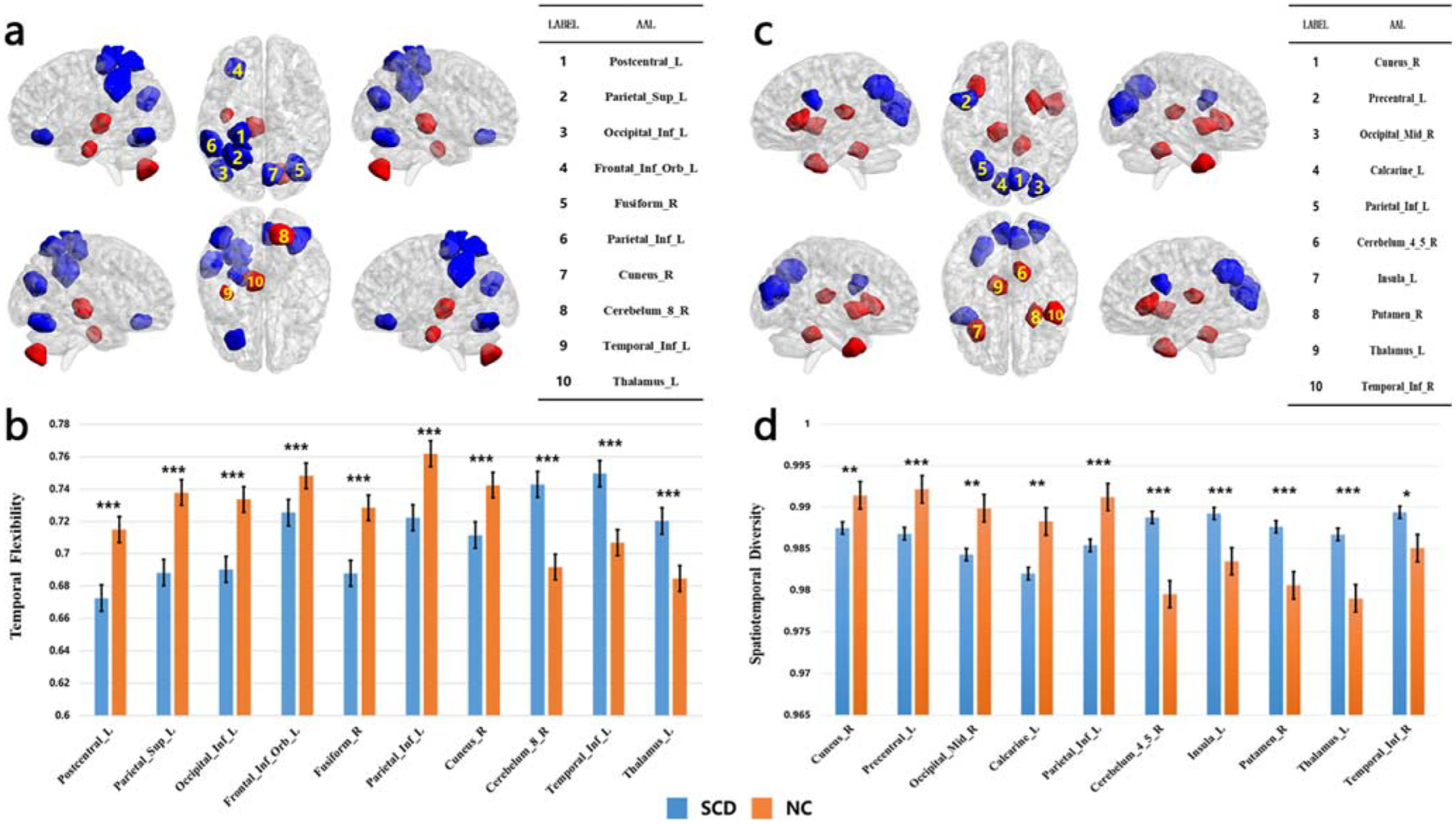
Top 10 regions with the largest weight of dynamic graph theoretic features. a Regions in red/blue each showed higher/lower mean temporal flexibility in SCD than in NC. b Bar plots of mean value of temporal flexibility of the top 10 brain regions, *** for P < 0.001; two sample t test. c Regions in red/blue each showed higher/lower mean spatiotemporal diversity in SCD than in NC. d Bar plots of mean value of spatiotemporal diversity of the top 10 brain regions, * for P < 0.05, ** for P < 0.01, *** for P < 0.001; two sample t test

For the spatiotemporal diversity, SCD was significantly lower in brain regions of Cuneus_R, Precentral_L, Occipital_Mid_R, Calcarine_L and Parietal_Inf_L than NC; and significantly higher in Cerebelum_4_5_R, Insula_L, Putamen_R, Thalamus_L and Temporal_Inf_R than NC. The results are shown in Fig. 4c and d.

Behavioral correlation

Pearson correlation was used to examine the relationship between the two dynamic graph theoretic measures and performance in neuropsychological tests, including the MMSE, AVLT-I, AVLT-D, AVLT-R, STT-A, STT-B, AFT, BNT, and MoCA-B. We used sex, age, years of education, GMV, HAMA and HAMD scores as covariates (Supplementary Table 1–2).

The results showed that, across SCD and NC, the temporal flexibility of Frontal_Inf_Orb_L was negatively correlated with AFT score (r = −0.223, P = 0.013, Fig. 5a). The temporal flexibility of Temporal_Inf_L was negatively correlated with BNT scores (r = −0.213, P = 0.018, Fig. 5b). The spatiotemporal diversity of Thalamus_L (aal) was negatively correlated with AVLT-I scores (r = −0.199, P = 0.027, Fig. 5c). All p values are corrected for false discovery rate. However, the SCD and NC did not differ in the slope of these regressions when examined in a slope test (all P’s > 0.2).

Fig. 5.

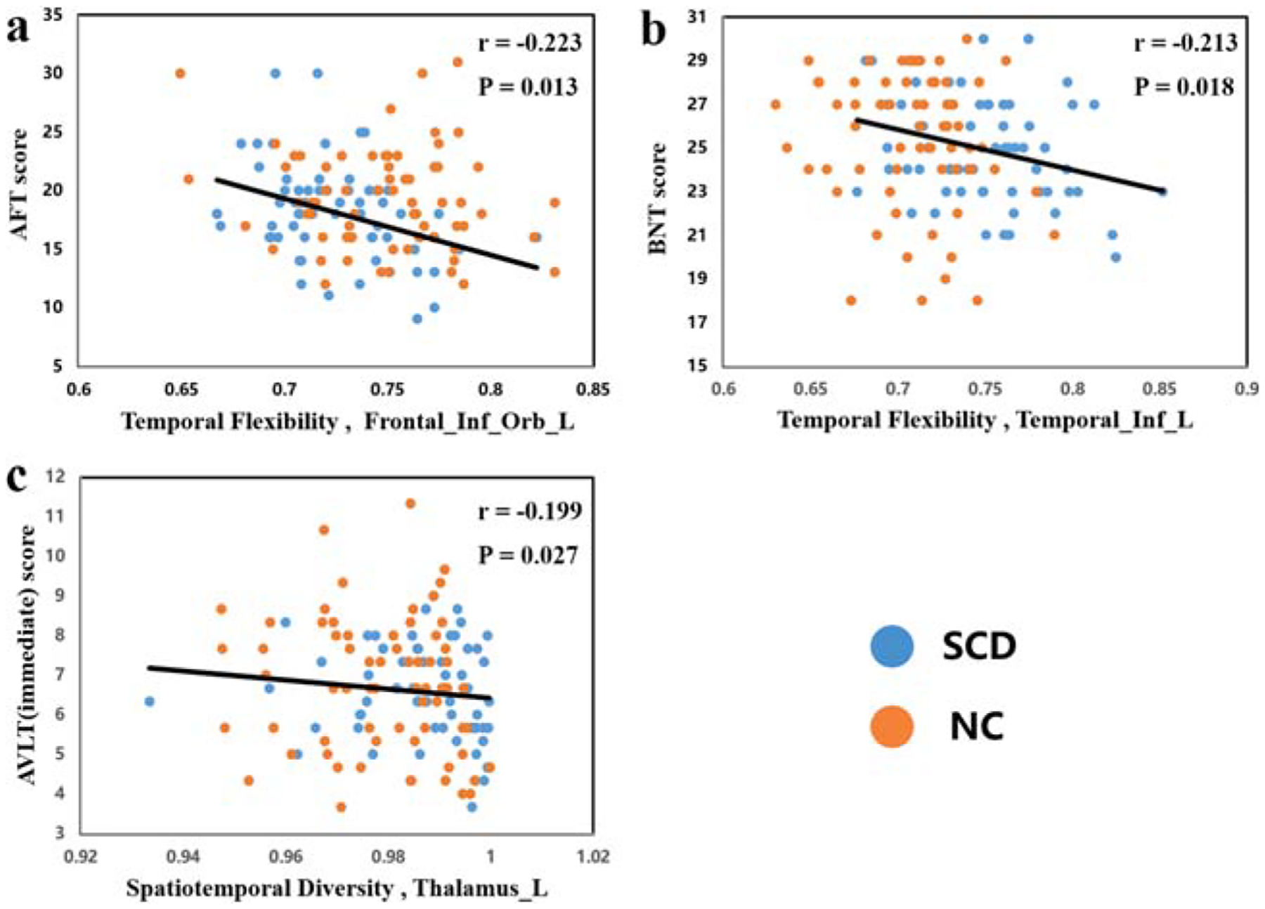
Behavioral correlation with dynamic graph theoretic parameters (FDR corrected, P < 0.05) across NC and SCD. NC: normal controls; SCD: subjective cognitive decline. AFT: animal fluency test; BNT: Boston naming test; AVLT: auditory verbal learning test

Discussion

In this study we quantified and compared the temporal flexibility and spatiotemporal diversity of cerebral dynamic functional connectivity in SCD and demographically matched NC. A SVM constructed of the feature classification matrix of temporal flexibility and spatiotemporal diversity achieved a mean group classification accuracy of 75.44% and 87.01%, respectively, much higher as compared to conventional static rs-fMRI metrics (44.5–51.2%) and structural morphometric measures (59.0%). Compared to NC, SCD demonstrated significantly different temporal flexibility and spatiotemporal diversity in the “top 10” brain regions that contributed to the classifier. The changes in these dynamic connectivity measures were related to cognitive performance: the temporal flexibility of the left inferior orbital frontal gyrus was negatively correlated with test score of AFT; temporal flexibility of the left inferior temporal lobe was negatively correlated with BNT scores; and spatiotemporal diversity of the left thalamus was negatively correlated with the AVLT-I score. Together, these results support dynamic network dysfunction as a new neural biomarker of the earliest stage of AD.

Classification accuracy

The classification accuracy constructed by matrix of the temporal flexibility and the spatiotemporal diversity was up to 95%, and the average accuracy of different dimensions was also above 75%. Thus, dynamic graph theoretic features best distinguished SCD from NC. Extant studies have examined brain network organization in a static, time-averaged manner under the assumption that functional interactions are stationary over time (Allen et al. 2014; Bassett et al. 2013; Damaraju et al. 2014; Hyett et al. 2015). The classification accuracy of the static graph theoretic parameters is lower than dynamic parameters as microscopic changes of brain states cannot be elucidated by time-averaged analyses (Calhoun et al. 2014; Hutchison et al. 2013; Zalesky et al. 2014). The current results are consistent with these earlier findings.

Dynamic graph theoretic measures perform better than static graph theoretic measures in classification, likely owing to the following reasons. First, cognitive processing requires an integrated activation of multiple intrinsic networks (Cohen and D’Esposito 2016). Dynamic neural features may capture the coordinated activation of different networks with faster timescales, while the static features are blind to these properties (Cohen 2018; Liegeois et al. 2017). Moreover, the dynamic graph theoretic measures reflect global information flow of the whole brain (Liegeois and Li 2019). The dynamic features can be regard as characterizing the temporal evolution or a special connectome of brain activities to support complex cognitive processes (van den Heuvel et al. 2016). Finally, research has shown that dynamic functional connectivity encode significantly more behavioral information than static functional connectivity metric (Liegeois and Li 2019). Further research is warranted to examine the roles of dynamic connectivities in cognition.

Analysis of dynamic connectivity has the potential to provide novel insights into brain function and dysfunction (Bassett et al. 2011; Bassett et al. 2015; Mattar et al. 2015; Braun et al. 2015). We systematically quantified large-scale brain dynamics in a large set of brain regions critical to various domains of cognition (Dosenbach et al. 2006; Power et al. 2013). We analyzed dynamic functional connectivity by focusing on temporal excursions of each brain region from its static network configuration (Calhoun et al. 2014; Hutchison et al. 2013; Allen et al. 2014). First, we identified the stable features related to dynamic patterns of time-varying connectivity by computing the temporal co-occurrence matrix. Second, we measured how frequently the brain region interacts with other brain regions in terms of temporal flexibility, which reflects the frequency at which a brain region interacts with regions belonging to other communities across time. Third, we identified the spatiotemporal diversity of each brain region with an entropy-based measure of how uniformly it interacts with regions in other communities. Spatiotemporal diversity provides complementary information about the spatial distribution of time-varying functional connectivity and captures subtle variations in brain function (Chen et al. 2016a). Finally, we used Lasso sparse algorithm to remove irrelevant features, and highlighted brain regions with obvious functional changes. The sparse algorithm was used to reduce the dimension of the features and avoid model over-fitting. The high classification accuracy of temporal flexibility and spatiotemporal diversity demonstrated the sensitivity and specificity of dynamic spatiotemporal properties in the identification of SCD from NC. Dynamic connectivity measures reflect brain changes in time and space simultaneously and distinguished SCD from NC with highest accuracy.

Brain regions with altered dynamic connectivity in SCD

The left inferior orbital frontal gyrus (IOFG) showed significant decreases in temporal flexibility and spatiotemporal diversity in SCD as compared to NC, suggesting that the connections between the left IOFG and other modules were disrupted at this very early stage of AD. The decline in spatiotemporal diversity indicated a decreasing number of modules in SCD (10 vs. 13 in NC), which may suggest an functional aggregation of brain regions in bigger, more centralized modules in SCD. The left IOFG is involved in syntactic processing, executive function and working memory (James et al. 2014; Harms et al. 2013; Melrose et al. 2009). Partaking in various cognitive processes, the OFG was reported to show disrupted connectivity in SCD in diffusion MRI research (Shu et al. 2018). The left OFG as well as the left inferior parietal lobe and left inferior temporal cortex that showed disruption appear to overlap with hubs and regions that manifest AD pathology (Buckner et al. 2009). These findings are reminiscent of the decreases in modularity, characterized by groups of regions densely connected among themselves and sparsely linked to regions outside the groups, in aMCI (Wang et al. 2013). The temporal flexibility of the left IOFG was negatively correlated with AFT scores, suggesting that the tendency of centralization as a (albeit partial) compensatory (Barulli and Stern 2013) or scaffolding (Park and Reuter-Lorenz 2009) mechanism to support verbal fluency. It thus appears that a greater level of concentricity across brain regions may be related to more significant prodromal AD pathology.

The left thalamus and left inferior temporal lobe both showed elevated temporal flexibility and spatiotemporal diversity, suggesting an increase in connectivity and connectivity modules, in SCD. AD pathology affected primary task-related networks (modules), potentially necessitating the use of additional networks (modules) in behavioral compensation (Barulli and Stern 2013). More brain regions were recruited to support cognitive performance where the primary module involved were subject to AD-related pathologies. From the perspective of correlation analysis, higher activation and more modules were beneficial to maintaining cognitive functions. Therefore, although the total number of modules was decreased in SCD, the objective neuropsychological test scores of SCD were still within the normal range. The negative correlations were consistent with an overall tendency toward cognitive decline in SCD, as would be expected of this population. Increased brain connectivity between posterior default mode regions were detected in SCD with a family history of AD and correlated with a reduced rate of cognitive performance over time (Verfaillie et al. 2018). These findings together are consistent with previous reports of co-existence of functional disruption and compensation in SCD (Yan et al. 2018; Yang et al. 2018).

When examining both the temporal flexibility and spatiotemporal diversity of the top 10 regions with the largest weight of dynamic graph theoretic features, we can see that several brain regions presented increases in both metrics, including the right cerebellum, left thalamus, and inferior temporal gyrus, and others decreases in both metrics, including the right cuneus, left inferior parietal lobe, and left frontal lobe. The former may represent enhanced connectivity features for functional compensation, whereas the latter may reflect loss of these features as a result of AD-related pathology (Hillary et al. 2006; Brenner et al. 2018). General “diffusion” of connectivity across brain regions may serve to mitigate the influences of single regions in a module on cognition (Brenner et al. 2018). For instance, individuals with aMCI showed disruptions in functional coupling between frontal and parietal regions and the positive frontal connectivity with default mode network may help preserve memory performance (Dillen et al. 2017). The current finding thus adds to this emerging literature and suggests dynamic connectivities as a central feature of functional brain re-organization during early development of AD.

Limitations of the study and conclusions

Several limitations should be considered. First, this is a cross-sectional study, and it remains unclear whether or how the findings observed of the SCD may predict the onset of MCI or AD. Further, longitudinal imaging would be required to describe how changes of dynamic functional connectivities of SCD affect the progression of the disease. Second, our research is based on single features. Future work is needed to understand how a combination of multiple features may help understand brain dynamics prodromal to the development of AD.

In conclusion, the study demonstrated altered spatiotemporal diversity and temporal flexibility in correlation with cognitive changes in SCD. The findings provided evidence for dynamic brain network dysfunction in the early stage of AD. The classifier comprised spatiotemporal connectivity features beyond those that can be captured by static network properties. The findings highlight the utility of dynamic graphic measures in detecting cerebral changes that may precede the onset of AD.

Abbreviations

AD

Alzheimer’s disease

SCD

Subjective cognitive decline

rs-fMRI

Resting-state functional magnetic resonance imaging

NC

Normal controls

aMCI

Amnestic mild cognitive impairment

BOLD

Blood oxygenation level-dependent

SVM

Support vector machines

HAMD

Hamilton depression rating scale

AVLT-H

Auditory Verbal Learning Test – HuaShan version

AFT

Animal Fluency Test

BNT

Boston Naming Test

STT-A

Shape Trails Test Parts A

STT-B

Shape Trails Test Parts B

MMSE

Mini–Mental State Examination

MoCA-B

Montreal Cognitive Assessment-basic

MES

Memory and executive function screening instrument

FAQ

Functional Activities Questionnaire

GDS

Geriatric Depression Scale

HAMA

Hamilton Anxiety Scale

NPI

Neuropsychiatric Inventory

GMV

Grey matter volume

TIV

Total intracranial volume

ROC

Receiver operating characteristic

AUC

The area under the receiver operating characteristic curve

ANCOVA

Analysis of covariance

FDR

False discovery rate

AVLT-I

AVLT-immediate recall

AVLT-D

AVLT-delayed recall

AVLT-R

AVLT-recognition recall

References

- Allen EA, Damaraju E, Plis SM, Erhardt EB, Eichele T, & Calhoun VD (2014). Tracking whole-brain connectivity dynamics in the resting state. Cerebral Cortex, 24(3), 663–676. 10.1093/cercor/bhs352. [DOI] [PMC free article] [PubMed] [Google Scholar]
- Ashburner J, & Friston KJ (1999). Nonlinear spatial normalization using basis functions. Human Brain Mapping, 7(4), 254–266. 10.1002/(SICI)1097-0193(1999)7:43.3.CO;2-7. [DOI] [PMC free article] [PubMed] [Google Scholar]
- Barulli D, & Stern Y (2013). Efficiency, capacity, compensation, maintenance, plasticity: Emerging concepts in cognitive reserve. Trends in Cognitive Sciences, 17(10), 502–509. 10.1016/j.tics.2013.08.012. [DOI] [PMC free article] [PubMed] [Google Scholar]
- Bassett DS, Wymbs NF, Porter MA, Mucha PJ, Carlson JM, & Grafton ST (2011). Dynamic reconfiguration of human brain networks during learning. Proceedings of the National Academy of Sciences of the United States of America, 108(18), 7641–7646. 10.1073/pnas.1018985108. [DOI] [PMC free article] [PubMed] [Google Scholar]
- Bassett DS, Wymbs NF, Rombach MP, Porter MA, Mucha PJ, & Grafton ST (2013). Task-based core-periphery organization of human brain dynamics. PLoS Computational Biology, 9(9), e1003171 10.1371/journal.pcbi.1003171. [DOI] [PMC free article] [PubMed] [Google Scholar]
- Bassett DS, Yang M, Wymbs NF, & Grafton ST (2015). Learning-induced autonomy of sensorimotor systems. Nature Neuroscience, 18(5), 744–751. 10.1038/nn.3993. [DOI] [PMC free article] [PubMed] [Google Scholar]
- Blondel VD, Guillaume JL, Lambiotte R, & Lefebvre E (2008). Fast unfolding of communities in large networks. Journal of Statistical Mechanics, 2008(10), 155–168. 10.1088/1742-5468/2008/10/p10008. [DOI] [Google Scholar]
- Braun U, Schäfer A, Walter H, Erk S, Romanczuk-Seiferth N, Haddad L, et al. (2015). Dynamic reconfiguration of frontal brain networks during executive cognition in humans. Proceedings of the National Academy of Sciences, 112(37), 11678–11683. 10.1073/pnas.1422487112. [DOI] [PMC free article] [PubMed] [Google Scholar]
- Brenner EK, Hampstead BM, Grossner EC, Bernier RA, Gilbert N, Sathian K, et al. (2018). Diminished neural network dynamics in amnestic mild cognitive impairment. International Journal of Psychophysiology, 130, 63–72. 10.1016/j.ijpsycho.2018.05.001. [DOI] [PMC free article] [PubMed] [Google Scholar]
- Bressler SL, & Menon V (2010). Large-scale brain networks in cognition: Emerging methods and principles. Trends in Cognitive Sciences, 14(6), 277–290. 10.1016/j.tics.2010.04.004. [DOI] [PubMed] [Google Scholar]
- Buckner RL, Sepulcre J, Talukdar T, Krienen FM, Liu H, Hedden T, et al. (2009). Cortical hubs revealed by intrinsic functional connectivity: Mapping, assessment of stability, and relation to Alzheimer’s disease. Journal of Neuroscience, 29(6), 1860–1873. 10.1523/jneurosci.5062-08.2009. [DOI] [PMC free article] [PubMed] [Google Scholar]
- Calhoun VD, Miller R, Pearlson G, & Adali T (2014). The chronnectome: Time-varying connectivity networks as the next frontier in fMRI data discovery. Neuron, 84(2), 262–274. 10.1016/j.neuron.2014.10.015. [DOI] [PMC free article] [PubMed] [Google Scholar]
- Chang C, & Glover GH (2010). Time-frequency dynamics of resting-state brain connectivity measured with fMRI. NeuroImage, 50(1), 81–98. 10.1016/j.neuroimage.2009.12.011. [DOI] [PMC free article] [PubMed] [Google Scholar]
- Chang CC, & Lin CJ (2011). LIBSVM: A library for support vector machines. [article]. ACM Transactions on Intelligent Systems and Technology, 2(3), 27 10.1145/1961189.1961199. [DOI] [Google Scholar]
- Chen, Cai W, Ryali S, Supekar K, & Menon V (2016a). Distinct global brain dynamics and spatiotemporal Organization of the Salience Network. PLoS Biology, 14(6), e1002469 10.1371/journal.pbio.1002469. [DOI] [PMC free article] [PubMed] [Google Scholar]
- Chen, Xu Y, Chu AQ, Ding D, Liang XN, Nasreddine ZS, et al. (2016b). Validation of the Chinese version of Montreal cognitive assessment basic for screening mild cognitive impairment. Journal of the American Geriatrics Society, 64(12), e285–e290. 10.1111/jgs.14530. [DOI] [PubMed] [Google Scholar]
- Cohen JR (2018). The behavioral and cognitive relevance of time-varying, dynamic changes in functional connectivity. NeuroImage, 180(Pt B), 515–525. 10.1016/j.neuroimage.2017.09.036. [DOI] [PMC free article] [PubMed] [Google Scholar]
- Cohen JR, & D’Esposito M (2016). The segregation and integration of distinct brain networks and their relationship to cognition. The Journal of Neuroscience, 36(48), 12083–12094. 10.1523/jneurosci.2965-15.2016. [DOI] [PMC free article] [PubMed] [Google Scholar]
- Cummings JL (1997). The neuropsychiatric inventory: Assessing psychopathology in dementia patients. Neurology, 48(5 Suppl 6), S10–S16. 10.1212/wnl.48.5_suppl_6.10s. [DOI] [PubMed] [Google Scholar]
- Damaraju E, Allen EA, Belger A, Ford JM, McEwen S, Mathalon DH, et al. (2014). Dynamic functional connectivity analysis reveals transient states of dysconnectivity in schizophrenia. Neuroimage Clin, 5, 298–308. 10.1016/j.nicl.2014.07.003. [DOI] [PMC free article] [PubMed] [Google Scholar]
- de Lacy N, Doherty D, King BH, Rachakonda S, & Calhoun VD (2017). Disruption to control network function correlates with altered dynamic connectivity in the wider autism spectrum. Neuroimage Clin, 15, 513–524. 10.1016/j.nicl.2017.05.024. [DOI] [PMC free article] [PubMed] [Google Scholar]
- Dillen KNH, Jacobs HIL, Kukolja J, Richter N, von Reutern B, Onur OA, et al. (2017). Functional disintegration of the default mode network in prodromal Alzheimer’s disease. Journal of Alzheimer’s Disease, 59(1), 169–187. 10.3233/JAD-161120. [DOI] [PubMed] [Google Scholar]
- Dosenbach NU, Visscher KM, Palmer ED, Miezin FM, Wenger KK, Kang HC, et al. (2006). A core system for the implementation of task sets. Neuron, 50(5), 799–812. 10.1016/j.neuron.2006.04.031. [DOI] [PMC free article] [PubMed] [Google Scholar]
- Finn ES, Shen X, Scheinost D, Rosenberg MD, Huang J, Chun MM, et al. (2015). Functional connectome fingerprinting: Identifying individuals using patterns of brain connectivity. Nature Neuroscience, 18(11), 1664–1671. 10.1038/nn.4135. [DOI] [PMC free article] [PubMed] [Google Scholar]
- Fornito A, Harrison BJ, Zalesky A, & Simons JS (2012). Competitive and cooperative dynamics of large-scale brain functional networks supporting recollection. Proceedings of the National Academy of Sciences, 109(31), 12788–12793. 10.1073/pnas.1204185109. [DOI] [PMC free article] [PubMed] [Google Scholar]
- Friston KJ, Holmes AP, Poline JB, Grasby PJ, Williams SCR, Frackowiak RSJ, et al. (1995). Analysis of fMRI time-series revisited. NeuroImage, 2(1), 45–53. 10.1006/nimg.1995.1023. [DOI] [PubMed] [Google Scholar]
- Genin E, Hannequin D, Wallon D, Sleegers K, Hiltunen M, Combarros O, et al. (2011). APOE and Alzheimer disease: A major gene with semi-dominant inheritance. [article]. Molecular Psychiatry, 16(9), 903–907. 10.1038/mp.2011.52. [DOI] [PMC free article] [PubMed] [Google Scholar]
- Guo QH, Zhou B, Zhao QH, Wang B, & Hong Z (2012). Memory and executive screening (MES): A brief cognitive test for detecting mild cognitive impairment. BMC Neurology, 12, 119 10.1186/1471-2377-12-119. [DOI] [PMC free article] [PubMed] [Google Scholar]
- Gusnard DA, Raichle ME, & Raichle ME (2001). Searching for a baseline: Functional imaging and the resting human brain. Nature Reviews. Neuroscience, 2(10), 685–694. 10.1038/35094500. [DOI] [PubMed] [Google Scholar]
- Hamilton M (1959). The assessment of anxiety states by rating. The British Journal of Medical Psychology, 32(1), 50–55. 10.1111/j.2044-8341.1959.tb00467.x. [DOI] [PubMed] [Google Scholar]
- Hamilton M (1960). A rating scale for depression. Journal of Neurology, Neurosurgery, and Psychiatry, 23, 56–62. 10.1136/jnnp.23.1.56. [DOI] [PMC free article] [PubMed] [Google Scholar]
- Harms MP, Wang L, Csernansky JG, & Barch DM (2013). Structure-function relationship of working memory activity with hippocampal and prefrontal cortex volumes. Brain Structure & Function, 218(1), 173–186. 10.1007/s00429-012-0391-8. [DOI] [PMC free article] [PubMed] [Google Scholar]
- Hillary FG, Genova HM, Chiaravalloti ND, Rypma B, & DeLuca J (2006). Prefrontal modulation of working memory performance in brain injury and disease. Human Brain Mapping, 27(11), 837–847. 10.1002/hbm.20226. [DOI] [PMC free article] [PubMed] [Google Scholar]
- Hutchison RM, Womelsdorf T, Allen EA, Bandettini PA, Calhoun VD, Corbetta M, et al. (2013). Dynamic functional connectivity: Promise, issues, and interpretations. NeuroImage, 80, 360–378. 10.1016/j.neuroimage.2013.05.079. [DOI] [PMC free article] [PubMed] [Google Scholar]
- Hyett MP, Breakspear MJ, Friston KJ, Guo CC, & Parker GB (2015). Disrupted effective connectivity of cortical systems supporting attention and interoception in melancholia. JAMA Psychiatry, 72(4), 350–358. 10.1001/jamapsychiatry.2014.2490. [DOI] [PubMed] [Google Scholar]
- James CE, Oechslin MS, Van De Ville D, Hauert CA, Descloux C, & Lazeyras F (2014). Musical training intensity yields opposite effects on grey matter density in cognitive versus sensorimotor networks. Brain Structure & Function, 219(1), 353–366. 10.1007/s00429-013-0504-z. [DOI] [PubMed] [Google Scholar]
- Jessen F, Amariglio RE, van Boxtel M, Breteler M, Ceccaldi M, Chetelat G, et al. (2014). A conceptual framework for research on subjective cognitive decline in preclinical Alzheimer’s disease. Alzheimers Dement, 10(6), 844–852. 10.1016/j.jalz.2014.01.001. [DOI] [PMC free article] [PubMed] [Google Scholar]
- Kaiser RH, Whitfield-Gabrieli S, Dillon DG, Goer F, Beltzer M, Minkel J, et al. (2016). Dynamic resting-state functional connectivity in major depression. Neuropsychopharmacology, 41(7), 1822–1830. 10.1038/npp.2015.352. [DOI] [PMC free article] [PubMed] [Google Scholar]
- Kang J, Wang L, Yan C, Wang J, Liang X, & He Y (2011). Characterizing dynamic functional connectivity in the resting brain using variable parameter regression and Kalman filtering approaches. NeuroImage, 56(3), 1222–1234. 10.1016/j.neuroimage.2011.03.033. [DOI] [PubMed] [Google Scholar]
- Kim J, Criaud M, Cho SS, Diez-Cirarda M, Mihaescu A, Coakeley S, et al. (2017). Abnormal intrinsic brain functional network dynamics in Parkinson’s disease. Brain, 140(11), 2955–2967. 10.1093/brain/awx233. [DOI] [PMC free article] [PubMed] [Google Scholar]
- Liegeois R, & Li J (2019). Resting brain dynamics at different time-scales capture distinct aspects of human behavior. 10(1), 2317, 10.1038/s41467-019-10317-7. [DOI] [PMC free article] [PubMed] [Google Scholar]
- Liegeois R, Laumann TO, Snyder AZ, Zhou J, & Yeo BTT (2017). Interpreting temporal fluctuations in resting-state functional connectivity MRI. NeuroImage, 163, 437–455. 10.1016/j.neuroimage.2017.09.012. [DOI] [PubMed] [Google Scholar]
- Liu J, Liao X, Xia M, & He Y (2018). Chronnectome fingerprinting: Identifying individuals and predicting higher cognitive functions using dynamic brain connectivity patterns. Human Brain Mapping, 39(2), 902–915. 10.1002/hbm.23890. [DOI] [PMC free article] [PubMed] [Google Scholar]
- Mattar MG, Cole MW, Thompson-Schill SL, & Bassett DS (2015). A functional cartography of cognitive systems. PLoS Computational Biology, 11(12), e1004533 10.1371/journal.pcbi.1004533. [DOI] [PMC free article] [PubMed] [Google Scholar]
- McDade E, & Bateman RJ (2017). Stop Alzheimer’s before it starts. Nature, 547(7662), 153–155. 10.1038/547153a. [DOI] [PubMed] [Google Scholar]
- Melrose RJ, Campa OM, Harwood DG, Osato S, Mandelkern MA, & Sultzer DL (2009). The neural correlates of naming and fluency deficits in Alzheimer’s disease: An FDG-PET study. International Journal of Geriatric Psychiatry, 24(8), 885–893. 10.1002/gps.2229. [DOI] [PMC free article] [PubMed] [Google Scholar]
- Menon V, & Uddin LQ (2010). Saliency, switching, attention and control: A network model of insula function. Brain Structure & Function, 214(5–6), 655–667. 10.1007/s00429-010-0262-0. [DOI] [PMC free article] [PubMed] [Google Scholar]
- Morgan VL, Abou-Khalil B, & Rogers BP (2015). Evolution of functional connectivity of brain networks and their dynamic interaction in temporal lobe epilepsy. Brain Connectivity, 5(1), 35–44. 10.1089/brain.2014.0251. [DOI] [PMC free article] [PubMed] [Google Scholar]
- Mucha PJ, Richardson T, Macon K, Porter MA, & Onnela J-P (2010). Community structure in time-dependent, multiscale, and multiplex networks. Science, 328(5980), 876–878. 10.1126/science.1184819. [DOI] [PubMed] [Google Scholar]
- Newman ME (2004). Fast algorithm for detecting community structure in networks. Physical Review. E, Statistical, Nonlinear, and Soft Matter Physics, 69(6 Pt 2), 066133 10.1103/PhysRevE.69.066133. [DOI] [PubMed] [Google Scholar]
- Park DC, & Reuter-Lorenz P (2009). The adaptive brain: Aging and neurocognitive scaffolding. Annual Review of Psychology, 60, 173–196. 10.1146/annurev.psych.59.103006.093656. [DOI] [PMC free article] [PubMed] [Google Scholar]
- Patterson C (2018). The World Alzheimer report 2018-the state of the art of dementia research: new frontiers. Alzheimer’s Disease International. [Google Scholar]
- Pfeffer RI, Kurosaki TT, Harrah CH Jr., Chance JM, & Filos S (1982). Measurement of functional activities in older adults in the community. Journal of Gerontology, 37(3), 323–329. 10.1093/geronj/37.3.323. [DOI] [PubMed] [Google Scholar]
- Power JD, Cohen AL, Nelson SM, Wig GS, Barnes KA, Church JA, et al. (2011). Functional network organization of the human brain. Neuron, 72(4), 665–678. 10.1016/j.neuron.2011.09.006. [DOI] [PMC free article] [PubMed] [Google Scholar]
- Power JD, Schlaggar BL, Lessov-Schlaggar CN, & Petersen SE (2013). Evidence for hubs in human functional brain networks. Neuron, 79(4), 798–813. 10.1016/j.neuron.2013.07.035. [DOI] [PMC free article] [PubMed] [Google Scholar]
- Rabin LA, Smart CM, & Amariglio RE (2017). Subjective cognitive decline in preclinical Alzheimer’s disease. Annual Review of Clinical Psychology, 13, 369–396. 10.1146/annurevclinpsy-032816-045136. [DOI] [PubMed] [Google Scholar]
- Rubinov M, & Sporns O (2010). Complex network measures of brain connectivity: Uses and interpretations. NeuroImage, 52(3), 1059–1069. 10.1016/j.neuroimage.2009.10.003. [DOI] [PubMed] [Google Scholar]
- Scheltens P, Blennow K, Breteler MMB, de Strooper B, Frisoni GB, Salloway S, et al. (2016). Alzheimer’s disease. The Lancet, 388(10043), 505–517. 10.1016/s0140-6736(15)01124-1. [DOI] [PubMed] [Google Scholar]
- Shu N, Liang Y, Li H, Zhang J, Li X, Wang L, et al. (2012). Disrupted topological organization in white matter structural networks in amnestic mild cognitive impairment: Relationship to sub-type. Radiology, 265(2), 518 10.1148/radiol.2112361. [DOI] [PubMed] [Google Scholar]
- Shu N, Wang X, Bi Q, Zhao T, & Han Y (2018). Disrupted topologic efficiency of white matter structural connectome in individuals with subjective cognitive decline. Radiology, 286(1), 229–238. 10.1148/radiol.2017162696. [DOI] [PubMed] [Google Scholar]
- Sperling RA, Aisen PS, Beckett LA, Bennett DA, Craft S, Fagan AM, et al. (2011). Toward defining the preclinical stages of Alzheimer’s disease: Recommendations from the National Institute on Aging-Alzheimer’s Association workgroups on diagnostic guidelines for Alzheimer’s disease. Alzheimers Dement, 7(3), 280–292. 10.1016/j.jalz.2011.03.003. [DOI] [PMC free article] [PubMed] [Google Scholar]
- Taghia J, Cai W, Ryali S, Kochalka J, Nicholas J, Chen T, et al. (2018). Uncovering hidden brain state dynamics that regulate performance and decision-making during cognition. Nature Communications, 9(1), 2505 10.1038/s41467-018-04723-6. [DOI] [PMC free article] [PubMed] [Google Scholar]
- Thompson GJ, Magnuson ME, Merritt MD, Schwarb H, Pan WJ, McKinley A, et al. (2013). Short-time windows of correlation between large-scale functional brain networks predict vigilance intraindividually and interindividually. Human Brain Mapping, 34(12), 3280–3298. 10.1002/hbm.22140. [DOI] [PMC free article] [PubMed] [Google Scholar]
- van den Heuvel MP, Bullmore ET, & Sporns O (2016). Comparative Connectomics. Trends in Cognitive Sciences, 20(5), 345–361. 10.1016/j.tics.2016.03.001. [DOI] [PubMed] [Google Scholar]
- Verfaillie SCJ, Pichet Binette A, Vachon-Presseau E, Tabrizi S, Savard M, Bellec P, et al. (2018). Subjective cognitive decline is associated with altered default mode network connectivity in individuals with a family history of Alzheimer’s disease. Biol Psychiatry Cogn Neurosci Neuroimaging, 3(5), 463–472. 10.1016/j.bpsc.2017.11.012. [DOI] [PubMed] [Google Scholar]
- Viviano RP, Hayes JM, Pruitt PJ, Fernandez ZJ, van Rooden S, van der Grond J, et al. (2018). Aberrant memory system connectivity and working memory performance in subjective cognitive decline. NeuroImage, 2019: 556–564. 10.1016/j.neuroimage.2018.10.015. [DOI] [PubMed] [Google Scholar]
- Wang J, Zuo X, Dai Z, Xia M, Zhao Z, Zhao X, et al. (2013). Disrupted functional brain connectome in individuals at risk for Alzheimer’s disease. Biological Psychiatry, 73(5), 472–481. 10.1016/j.biopsych.2012.03.026. [DOI] [PubMed] [Google Scholar]
- Wang J, Wang X, Xia M, Liao X, Evans A, & He Y (2015). GRETNA: A graph theoretical network analysis toolbox for imaging connectomics. Frontiers in Human Neuroscience, 9, 386 10.3389/fnhum.2015.00386. [DOI] [PMC free article] [PubMed] [Google Scholar]
- Yaesoubi M, Miller RL, Bustillo J, Lim KO, Vaidya J, & Calhoun VD (2017). A joint time-frequency analysis of resting-state functional connectivity reveals novel patterns of connectivity shared between or unique to schizophrenia patients and healthy controls. Neuroimage Clin, 15, 761–768. 10.1016/j.nicl.2017.06.023. [DOI] [PMC free article] [PubMed] [Google Scholar]
- Yan C-G, Wang X-D, Zuo X-N, & Zang Y-F (2016). DPABI: Data Processing & Analysis for (resting-state) brain imaging. [journal article]. Neuroinformatics, 14(3), 339–351. 10.1007/s12021-016-9299-4. [DOI] [PubMed] [Google Scholar]
- Yan T, Wang W, Yang L, Chen K, Chen R, & Han Y (2018). Rich club disturbances of the human connectome from subjective cognitive decline to Alzheimer’s disease. Theranostics, 8(12), 3237–3255. 10.7150/thno.23772. [DOI] [PMC free article] [PubMed] [Google Scholar]
- Yang L, Yan Y, Wang Y, Hu X, Lu J, Chan P, et al. (2018). Gradual disturbances of the amplitude of low-frequency fluctuations (ALFF) and fractional ALFF in Alzheimer Spectrum. Frontiers in Neuroscience, 12, 975 10.3389/fnins.2018.00975. [DOI] [PMC free article] [PubMed] [Google Scholar]
- Yesavage JA, Brink TL, Rose TL, Lum O, Huang V, Adey M, et al. (1982). Development and validation of a geriatric depression screening scale: A preliminary report. Journal of Psychiatric Research, 17(1), 37–49. 10.1016/0022-3956(82)90033-4. [DOI] [PubMed] [Google Scholar]
- Zalesky A, Fornito A, Cocchi L, Gollo LL, & Breakspear M (2014). Time-resolved resting-state brain networks. Proceedings of the National Academy of Sciences, 111(28), 10341–10346. 10.1073/pnas.1400181111. [DOI] [PMC free article] [PubMed] [Google Scholar]
- Zhang D, & Raichle ME (2010). Disease and the brain’s dark energy. Nature Reviews. Neurology, 6(1), 15–28. 10.1038/nrneurol.2009.198. [DOI] [PubMed] [Google Scholar]
- Zhang S, Ide JS, Hu S, Zhornitsky S, Wang W, et al. (2018). Dynamic network dysfunction in cocaine dependence: Graph theoretical metrics and stop signal reaction time. Neuroimage Clin, 18, 793–801. 10.1016/j.nicl.2018.03.016. [DOI] [PMC free article] [PubMed] [Google Scholar]
- Zhao Q, Guo Q, Li F, Zhou Y, Wang B, & Hong Z (2013). The Shape Trail test: Application of a new variant of the trail making test. PLoS One, 8(2), e57333 10.1371/journal.pone.0057333. [DOI] [PMC free article] [PubMed] [Google Scholar]
- Zhao Q, Guo Q, Liang X, Chen M, Zhou Y, Ding D, et al. (2015). Auditory verbal learning test is superior to Rey-Osterrieth complex figure memory for predicting mild cognitive impairment to Alzheimer’s disease. Current Alzheimer Research, 12(6), 520–526. 10.1016/j.jalz.2015.06.422. [DOI] [PubMed] [Google Scholar]
Associated Data
This section collects any data citations, data availability statements, or supplementary materials included in this article.