A unified framework for joint-tissue transcriptome-wide association and Mendelian Randomization analysis

Abstract

Here we present a Joint-Tissue Imputation (JTI) approach and a Mendelian Randomization (MR) framework for causal inference, MR-JTI. JTI borrows information across transcriptomes of different tissues, leveraging shared genetic regulation, to improve prediction performance in a tissue-dependent manner. Notably, JTI includes single-tissue imputation PrediXcan as a special case and outperforms other single-tissue approaches (BSLMM and Dirichlet Process Regression). MR-JTI models variant-level heterogeneity (primarily due to horizontal pleiotropy, addressing a major challenge of TWAS interpretation) and performs causal inference with type-I error control. We make explicit the connection between the genetic architecture of gene expression and of complex traits, and the suitability of MR as a causal inference strategy for TWAS. We provide a resource of imputation models generated from GTEx and PsychENCODE panels. Analysis of biobanks and meta-analysis data and extensive simulations show substantially improved statistical power, replication, and causal mapping rate for JTI relative to existing approaches.

The Genome-wide Association Studies (GWAS) methodology has substantially increased our understanding of the genetic basis of complex diseases. The reported enrichment of trait-associated loci in noncoding regions has promoted eQTL analyses and transcriptome-wide association studies (TWAS)^1–3, which explicitly exploit the fact that gene expression may be a molecular mediator between genotype and phenotype.

The power of TWAS / PrediXcan, a two-stage procedure, may be attributed to two factors. The first comes from the accuracy of the prediction model of gene expression. The second comes from the association between gene expression and phenotype. As GWAS meta-analyses continue to increase in sample size, the prediction quality remains a rate-limiting step. Improvement in the prediction quality should substantially increase the power of TWAS / PrediXcan. However, current approaches do not fully leverage the multi-tissue nature of transcriptome resources (Genotype-Tissue Expression [GTEx] project) and the comprehensive atlases of regulatory elements (ENCODE project or Roadmap Epigenomics). Conventional TWAS / PrediXcan generates the prediction model for a gene in each target tissue separately^1–3, ignoring the presence of tissue-shared genetic regulation. MultiXcan integrates information across multiple tissue studies to improve statistical power for association analysis by regressing the principal components of the predicted expression data across the tissues on the trait⁴. However, MultiXcan is a multi-tissue association analysis approach and does not aim to improve prediction of gene expression in each tissue; furthermore, the effect size and direction of each PC are not easily interpretable. UTMOST is a cross-tissue TWAS approach that aims to improve the prediction performance (through variable selection using a group penalty term)⁵. However, it does not leverage the similarity among tissues. Recent studies have shown that eQTL sharing among tissues is abundant^6–8, with stronger sharing among biologically-related tissues (e.g., the various brain regions)⁹. We hypothesize that, for any given tissue, we can improve prediction by leveraging other tissues with similar genetic regulation profile.

Here, we develop JTI, an extension of PrediXcan¹ that exploits the power of multi-tissue transcriptomes (the GTEx v8 panel¹⁰) and atlases of regulatory elements, to elucidate the genetic architecture of gene expression and to identify gene-level associations with complex traits. The method leverages the shared regulatory architecture of gene expression to substantially improve prediction. Prediction accuracy is evaluated in two external transcriptome datasets, demonstrating that JTI outperforms conventional PrediXcan and another multi-tissue imputation methodology UTMOST⁵. Application of JTI models to GWAS data and a biobank leads to replication of well-known gene-level associations and identifies novel associations that are specific to JTI.

Mendelian Randomization leverages genetic variation to make inferences about causality using observational data. Using multiple genetic variants, PrediXcan can be viewed as (two-sample) allele-score-based Mendelian Randomization^11,12 but without pleiotropy control (Extended Data Fig. 1). In Instrumental Variable (IV) analysis, three conditions¹³ are required for a model Z to be a valid instrument for estimating the causal effect of a gene G on the trait Y (Fig. 1): marginal relevance (i.e., Z is associated with G), confounder independence (i.e., Z is independent of a confounder U), and exclusion restriction (i.e., there is no direct effect of Z on Y which is not completely mediated by G). The causal inference of interest to us is G → Y. The presence of Z → Y other than through G would indicate the existence of a pleiotropic effect, violating exclusion restriction (Extended Data Fig. 1). The inverse-variance weighted (IVW) method provides a consistent estimate of causal effect when all the genetic variants used are valid IVs^14,15. Subsequently, MR-Egger¹⁶, weighted median¹⁷, MR-PRESSO¹⁸, and related approaches were developed to address (the pervasive) horizontal pleiotropy, which can lead to biased causal effect estimates, false-positive causal relationships, and loss of power. Under PrediXcan, the weighted allele score (i.e., the imputed genetically-determined expression), as an instrumental variable, may contain genetic variants with horizontal pleiotropic effects and thus result in a biased estimate of the causal effect of G on Y even if most of the variants are valid instruments. To address this major limitation, we provide an approach for jointly estimating the causal effect and the heterogeneity using summary statistics, thus incorporating Mendelian Randomization into JTI.

Fig. 1: The JTI framework: multi-tissue gene expression imputation model and causal inference engine.

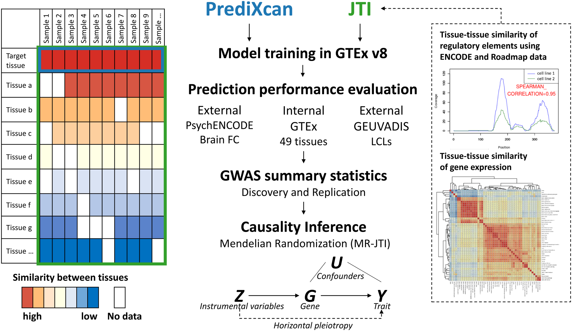
To improve imputation in a target tissue (blue box), JTI borrows information from the remaining tissues (green box) by leveraging tissue-tissue similarity from expression and epigenomic (e.g., ENCODE/Roadmap) profiles. For JTI, the prediction model is generated via cross-validation by solving an optimization problem (Methods) that incorporates data on gene expression similarity and DHS profile similarity across tissues. Prediction performance is assessed through cross-validation in GTEx and validation in additional external datasets (e.g., PsychENCODE and GEUVADIS). In trait mapping applications, prediction models can be applied to GWAS summary statistics to identify robust gene-level associations. Finally, causal effect inference is performed for each of the genes from the association analysis, using a novel summary statistics-based approach, MR-JTI. To this end, MR-JTI estimates the confounding due to invalid genetic instruments on the trait, providing an approximately unbiased causal effect estimate, and implements a statistical test of the null causal hypothesis. The LD contamination, a major challenge for TWAS, is addressed by a variable selection process to estimate the per-instrument contribution to heterogeneity (Methods).

RESULTS

Framework

Extending conventional PrediXcan¹, we developed a multi-tissue expression prediction framework (Fig. 1). PrediXcan generates prediction models using only the samples in the target tissue by solving a family of minimization problems (equation [1] in Methods). In contrast, JTI integrates all tissues through a loss function parameterized by a set of weights (i.e., weighted square error loss; equation [2] in Methods) in order to improve prediction performance in a target tissue, assigning higher weights to tissues with a greater degree of similarity and lower weights to tissues with a lower degree of similarity. A reference multi-tissue transcriptome panel (GTEx) was used to train models. For each target tissue, an optimization problem is solved (Methods) via cross-validation. Besides the within-reference-panel (GTEx) performance evaluation, we tested the models in external datasets (PsychENCODE for brain prefrontal cortex and GEUVADIS for lymphoblastoid cell lines [LCLs]). Methodological and performance comparisons were performed among PrediXcan, JTI, and UTMOST. We applied the models to GWAS data to identify gene-level associations and sought independent replication of results. We developed a causal inference engine MR-JTI, as an extension of JTI, that provides a unified framework for TWAS and (two-sample) Mendelian Randomization. MR-JTI estimates the overall heterogeneity, providing a way to address a major challenge of TWAS interpretation.

Similarity matrix

JTI exploits the shared genetic regulation of gene expression across tissues. The similarity matrix for expression profile was generated from the tissue-level expression Pearson correlation (Extended Data Fig. 2) and, for proof-of-principle, gene-level DNase I hypersensitive sites (DHS) similarity for each tissue-tissue pair (Methods). Weights used in the loss function were calculated as the product of power laws, one for the expression-based similarity and another for the DHS-profile-based similarity (data source: ENCODE and Roadmap; Methods). One feature of a power law, π(r) = r^m, that makes it attractive as a functional form for quantifying similarity is scale invariance; power laws with a predefined exponent are equivalent up to constant factors: π(cr) = c^mπ(r) ∝ π(r). The powers are considered hyper-parameters (with PrediXcan a special instance), and hyper-parameter tuning is performed for each gene by cross-validation (Methods).

Performance of JTI and single-tissue models

We compared the performance of JTI and PrediXcan as imputation methodologies using GTEx v8. On average, PrediXcan resulted in 6,842 imputable genes (“iGenes,” defined as genes with r > 0.1 and P < 0.05 from the correlation between predicted and observed expression) across the 49 tissues (Fig. 2a). The criterion r > 0.1, rather than r² > 0.01, was used to filter genes with a negative correlation between predicted and observed expression. The average number of iGenes, 10,527, was substantially higher with the application of JTI (Fig. 2a, Supplementary Table 1). On average, 92.9% of the PrediXcan-derived iGenes remained imputable under JTI (Fig. 2b). For tissues with more than 200 samples, 96.5% of the iGenes were captured by JTI. To further quantify the performance gain, we calculated the increase in the proportion of iGenes and the increase in r² (expression variance explained by local genetic variation), denoted by ΔpiG and Δr², respectively. The ΔpiG (mean = 60.3%) and Δr² (mean = 0.036) varied from tissue to tissue (Fig. 2c and Supplementary Table 1).

Fig. 2: Comparison of the prediction performance between PrediXcan and JTI.

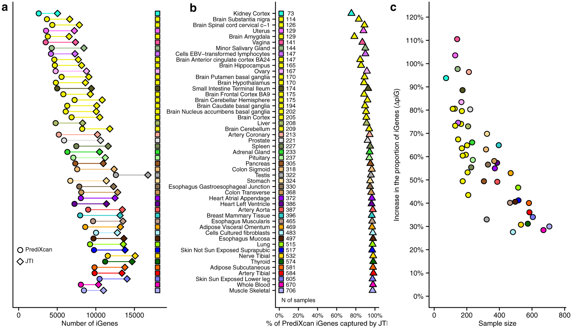
a, The number of imputable genes (iGenes) is greater for JTI than for PrediXcan in all GTEx (v8) tissues. b, Most (92.9% on average) of the iGenes under PrediXcan are also iGenes under JTI. c, The increase in the proportion of iGenes (ΔpiG) is negatively correlated (Spearman r = −0.80, P = 4.4e-12) with tissue sample size; thus, tissues with small sample sizes, which therefore have more to gain, tend to show higher ΔpiG. Tissue panels with more modest sample sizes can benefit more and indeed display greater performance gains under JTI. Tissue panels that have the largest sample sizes also show performance gains though less, as expected.

Tissues with small sample sizes tended to have greater gains in the proportion of imputable genes (Fig. 2c). Among the 49 tissues (Extended Data Fig. 3), the vagina tissue showed the highest performance gain (N = 141, ΔpiG =111.2%, Δr² = 0.050). Tissues with large sample sizes (e.g., whole blood, N = 670, ΔpiG = 27.7%, Δr² = 0.015) and tissues with highly specific genetic regulation or expression profile (e.g., testis, N = 322, ΔpiG = 32.8%, Δr² = 0.021), showed more limited gains. Thus, tissues with more modest sample sizes or those with some similarity with the other tissues are the ones likely to see greater gains from a multi-tissue model. Nevertheless, the performance gain from this model in all tissues was substantial.

We compared JTI with other single-tissue imputation approaches: the top eQTL; Bayesian Sparse Linear Mixed Model (BSLMM), and Dirichlet Process Regression (DPR)¹⁹ (Methods and Extended Data Fig. 4). JTI outperformed these single-tissue approaches, highlighting the performance gain from leveraging the cross-tissue information.

Prediction performance as a function of sample size

To assess the impact of sample size on imputation performance, we conducted a comparison of GTEx v6p and v8 models. Among the 44 overlapping tissues (average sample size N_v6p = 160, N_v8 = 332), the average number of iGenes increased from 4,570 (v6p) to 7,213 (v8) for PrediXcan and from 6,340 (v6p) to 10,969 (v8) for JTI, showing the substantial influence of sample size (Supplementary Table 1, Extended Data Fig. 5).

Comparison with existing joint-tissue methodologies

In addition to the multi-tissue feature, a distinctive feature of JTI is its integration of data on regulatory elements (extensible to functional genomic data [Methods]) from an epigenomic reference panel. We, therefore, evaluated JTI more fully through comparison with UTMOST (i.e., the Cross-Tissue gene Expression IMPutation [CTIMP] of the framework)⁵, which lacks the feature. We modified the UTMOST script after detecting artificially-inflated prediction performance in external datasets (Supplementary Note, Extended Data Fig. 6 and Extended Data Fig. 7). Throughout, “UTMOST” denotes the “modified UTMOST” unless explicitly noted (as “original UTMOST”).

We first evaluated the performance, in PsychENCODE data (brain prefrontal cortex, N = 415), of PrediXcan, UTMOST, and JTI models trained in GTEx v8 brain frontal cortex BA9 tissue. In comparison with the single-tissue PrediXcan (N_iGenes = 3,193), UTMOST (N_iGenes = 4,486) and JTI (N_iGenes = 5,417) identified more iGenes (r > 0.1 and P < 0.05) (Fig. 3a). Of the 3,193 PrediXcan-derived iGenes, 2,920 were captured by both UTMOST and JTI (Fig. 3b). In addition to the 2,920 iGenes, UTMOST and JTI identified 1,219 additional shared iGenes, showing the consistent improvement from a multi-tissue approach. KEGG pathway and Gene Ontology analysis showed that the 1,219 genes were significantly enriched in metabolic pathways (P = 2.80e-06) and membrane (P = 5.10e-05) (Supplementary Table 2). Notably, 1,110 JTI-specific iGenes were replicated in PsychENCODE, compared to 311 UTMOST-specific iGenes, underscoring the substantial gain in replication rate (measured in an external dataset) that can be attained through JTI. Fig. 3c and 3d show the shared and method-specific iGenes from all pairwise comparisons between the methodologies.

Fig. 3: Comparison of the performance of the various methods using external transcriptome data from GEUVADIS LCLs (a-d) and PsychENCODE prefrontal cortex tissues (e-h).

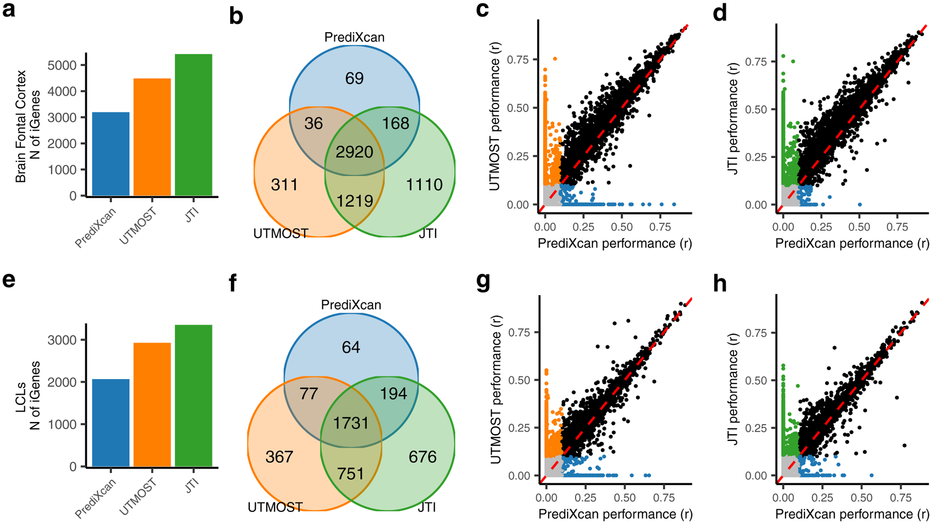
a, e, The Venn diagram plots show the overlap of the iGenes (defined by r > 0.1 and P < 0.05) from PrediXcan, UTMOST, and JTI. b, f, The bar plots of the number of iGenes using the different training models. c, d, g, h, The scatter plots of the correlation r between predicted and observed expression. Comparison of c, g, UTMOST and d, h, JTI with PrediXcan. The orange, green, and blue dots denote genes only imputable using UTMOST, JTI, and PrediXcan, respectively. The black and grey dots denote genes consistently imputable and not imputable, respectively, using both methods in the comparison. The specific training and test datasets used are shown on the left. Note, for example, that we used GTEx EBV-transformed lymphocytes as training set and GEUVADIS LCLs (a matched cell type) as test set in the bottom-half analyses.

Next, we conducted comparisons using GTEx v8 EBV-transformed lymphocytes as the training set and GEUVADIS LCLs data (N = 421) as the test set. In comparison with PrediXcan¹ (N_iGenes = 2,066), UTMOST (N_iGenes = 2,926) and JTI (N_iGenes = 3,352) identified more iGenes (Fig. 3e). UTMOST and JTI captured 87.5% and 93.2%, respectively (Fig. 3f, 3g, 3h), of the 2,066 PrediXcan-derived iGenes.

Type-I error and power analysis

Given the possibility of inflated type I error (e.g., due to shared samples across tissues), we conducted extensive simulations (see Supplementary Note) and found that JTI controls the type I error rate. Indeed, JTI, PrediXcan, and UTMOST displayed equivalent type I error rates (Extended Data Fig. 8 and Supplementary Table 3).

We also estimated their statistical power (see Supplementary Note). The predicted expression (i.e., genetically determined) levels were generated using actual empirical prediction performance (R²) values in the two external datasets (PsychENCODE [brain prefrontal cortex] and GEUVADIS [LCLs]) from the PrediXcan, UTMOST, and JTI models. Notably, the statistical power of JTI was substantially higher than that of UTMOST and PrediXcan across all sample sizes ranging from 5k to 500k (Extended Data Fig. 9) based on the PsychENCODE dataset. By comparison, based on the GEUVADIS dataset, JTI and UTMOST outperformed PrediXcan, with JTI showing a modest improvement in statistical power over UTMOST. Due to the availability of several brain regions in the GTEx resource, JTI benefits from leveraging tissue-similarity information across the relevant (brain) tissues, which may explain JTI’s substantial performance improvement. However, the reduced gain in power for JTI over UTMOST in LCLs may be due to the fact that gene expression in LCLs is more highly tissue-specific and, thus, JTI applied to this tissue has less to gain from leveraging tissue-similarity information.

Application to GWAS data

We applied PrediXcan and JTI models to a continuous trait, low-density lipoprotein cholesterol (LDL-C, quantile-transformed), from a GWAS (UK biobank LDL-C; N = 343,621) dataset (Methods, Fig. 4a). In general (Supplementary Fig. 1), the proportion of true positives π₁ was higher for JTI (0.251) than PrediXcan (0.232). PrediXcan and JTI identified 411 and 680 associations in liver, respectively (P_FDR < 0.05). Among the 411 PrediXcan significant genes (P_FDR < 0.05), 353 (85.9%) also showed nominal association under JTI (P < 0.05). Of the 411, nine were well-known lipid metabolism genes (Supplementary Table 4); JTI extended this number to seventeen (Fig. 4b). The SORT1-PSRC1-CELSR2 cluster, LPA, FADS1, KPNB1, and additional genes were found to be associated with LDL-C level using either PrediXcan or JTI (Supplementary Table 5). Within the well-known SORT1-PSRC1-CELSR2 cluster, JTI and PrediXcan showed similar association signals for the putatively causal gene SORT1. For KPNB1, JTI showed a boosted signal (P = 4.80e-14) relative to PrediXcan (P = 3.95e-09). One possible interpretation is the greater imputation quality (Fig. 5a and 5e) for JTI (r² = 5.16%) than for PrediXcan (r² = 1.91%). Similar levels of improvement were observed for ANGPTL3, PPARG, and LPA (Fig. 5b–5d and 5f–5h).

Fig. 4: Manhattan plot for LDL-C level from the application of PrediXcan and JTI models in liver to UK biobank LDL-C GWAS summary statistics.

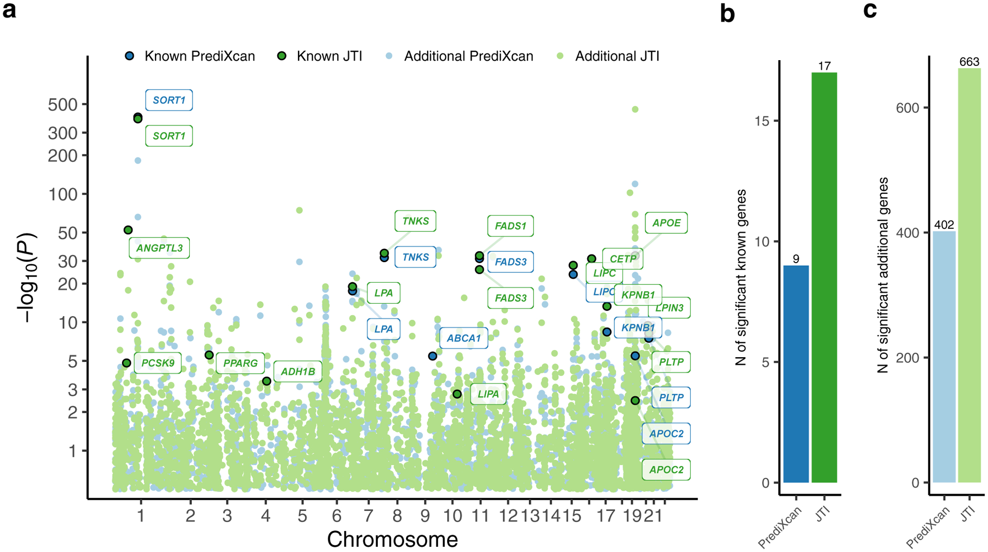
a, LDL-C TWAS Manhattan plot showing the association results from application of PrediXcan (blue) and JTI (green) models. The known genes (from the KEGG cholesterol metabolism pathway and the literature-based silver standard) and additional genes are shown in dark circle and light circle, respectively. Number of b, known genes and c, additional genes that were significantly associated (P_FDR < 0.05) with LDL-C. Except for ABCA1, all (eight) known genes found by PrediXcan (SORT1, LPA, TNKS, FASD3, LIPC, KPNB1, PLTP, and APOC2) were identified by JTI with greater or similar level of significance. JTI identified 8 additional known genes (ANGPTL3, LIPA, PPARG, CETP, etc.).

Fig. 5: Improved performance of JTI relative to PrediXcan in GTEx liver tissue for LDL-associated genes.

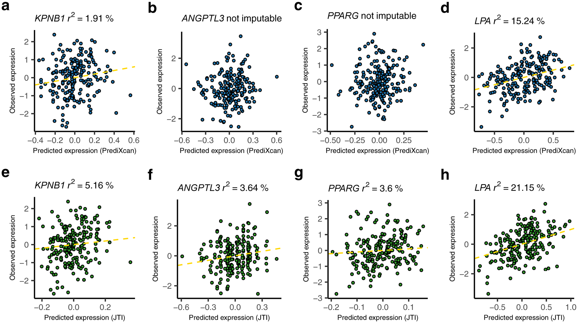
The upper scatter plots a, b, c, and d show the prediction performance for KPNB1, ANGPTL3, PPARG, and LPA, respectively, using PrediXcan. The bottom scatter plots e, f, g, and h show the JTI results, which outperform the corresponding PrediXcan results. (Here “not imputable” is defined as r < 0.1 [which implies r² < 0.01] or P > 0.05.) A regression line (shown as yellow dashed line) is included if the gene is imputable. LDL-C associated genes were identified using JTI or PrediXcan applied to UK biobank GWAS summary statistics.

JTI identified 328 additional associations (JTI P_FDR < 0.05, PrediXcan P > 0.05, Supplementary Table 5). The improved imputation quality for CETP (JTI: r² = 5.30%; PrediXcan: not imputable) and FADS1 (JTI: 10.06%; PrediXcan: not imputable), which were among the 328, likely contributed to the significant associations from JTI (P = 5.71e-32 and P = 9.19e-34 for CETP and FADS1, respectively). JTI identified some novel associations with LDL-C. A signal on CCDC92 (P = 7.14e-06) was amplified by JTI (P = 6.52e-08) via higher r² (JTI: 8.86%; PrediXcan: 2.46%). A genome-wide significant signal for POLK was identified only by JTI (P =3.49e-75). The association of POLK in liver was successfully replicated in both GLGC and BioVU (P = 5.70e-21 and P = 5.24e-03, Supplementary Table 6), with concordant direction of effect. The higher prediction quality of TIRAP resulted in a stronger association signal from JTI (r² = 5.33%, P = 7.10e-06) than PrediXcan (r² = 2.35%, P = 3.68e-03). The association between TIRAP and LDL-C was replicated in BioVU (P = 1.17e-02, Supplementary Table 6).

Performance comparison of PrediXcan and JTI was performed in additional GWAS datasets (Supplementary Table 7), including bipolar disorder, schizophrenia, blood glucose, HDL-C, Vitamin C, C-reactive protein, and creatinine, in relevant tissues. On average, PrediXcan and JTI identified 377.9 (range: 64 – 973) and 576.3 (range: 130 – 1192) significant genes (P_FDR < 0.05), respectively.

Causal effect inference and heterogeneity estimation

We observed that the Mendelian Randomization “model” (θ = αβ, where θ is the trait effect vector and β is the expression effect vector for the instruments, and α is the gene-level causal effect on the trait) describes the summary data (i.e., the genetic effects in GWAS and gene expression data) reasonably well. That is, the causal effect (of the gene on a complex trait) has a consistent magnitude across gene expression based genetic instruments for highly polygenic traits based on theoretical (Methods) and empirical grounds²⁰.

Our primary aim is gene prioritization and determination of gene causal effect on a trait. We provide a novel approach to causal inference (Methods) and highlight possible sources of bias (PSB), including unmeasured confounding, weak instrument bias (Supplementary Note), and invalid instruments due to horizontal pleiotropy. Extending JTI, the MR-JTI framework implements causal effect inference (Fig. 1, Extended Data Fig. 1). By modeling the heterogeneity (mainly involving horizontal pleiotropy), MR-JTI further helps prioritize genes (Methods).

We performed causal inference on the 680 genes in liver with a significant JTI association with LDL-C (JTI P_FDR < 0.05). Because of the generally modest sample size of transcriptome studies (e.g., compared to GWAS meta-analyses of complex traits), the genetic instruments may suffer from weak instrument bias (Supplementary Note); however, the F-statistic for JTI tended to be higher than for PrediXcan, driven by the higher variance in gene expression explained by the JTI models (Extended Data Fig. 3).

For each gene, we compared the MR-JTI estimate of the gene effect with the median estimator, i.e., the median of the Wald ratio estimates (a consistent estimator when less than half of IVs are invalid; Supplementary Note) across the cis-eQTLs (P_FDR < 0.05) (Extended Data Fig. 10). A significant positive correlation was observed (Spearman r = 0.65, P < 2.2e-16) in the actual data but no correlation from shuffled GWAS summary statistics (Extended Data Fig. 10). The LD-pruning at r² = 0.2 may still leave some underlying correlation. We therefore conducted MR-JTI based on LD pruning at r² = 0.01. The Pearson correlation (r) between the effect size (gene-level) using r² = 0.2 and using r² = 0.01 is 0.909.

MR-JTI identified 138 significant genes (based on Bonferroni adjustment) compared to 30 (4.41%) genes based on shuffled GWAS summary statistics. The well-studied gene SORT1 (Supplementary Fig. 2) and nearby co-expressed genes PSRC1 and CELSR2 showed significant association with LDL-C level after heterogeneity control. Furthermore, LPA, TNKS, FASD3, PLTP, and LPIN3 are additional well-known genes showing significant associations (Fig. 6; Supplementary Table 8). The expression of POLK, the replicated LDL-C-associated gene, attained positive correlation via MR-JTI, which indicates a putative causal role for POLK in lipid metabolism. The POLK protein (DNA polymerase kappa) performs DNA synthesis across damaged genomic DNA²¹. Copy loss or mutation of the gene has, in fact, been associated with impaired genome integrity and replication-independent repair²². DNA-damage-induced accumulation of senescent cells in tissues leads to chronic inflammation and impairment of glucose and lipid metabolism²³. Notably, significantly increased mutation frequencies have been observed globally in the liver tissue, an important site of cholesterol metabolism, in Polk −/− mice²⁴. Consistent with this connection between POLK’s role in DNA repair and lipid metabolism, other DNA-repair related genes (SIRT1, SIRT6, PARP1) have also been found to play a role in lipid and glucose metabolism²³.

Fig. 6: MR-JTI identifies LDL-C associated genes with potential causal effect.

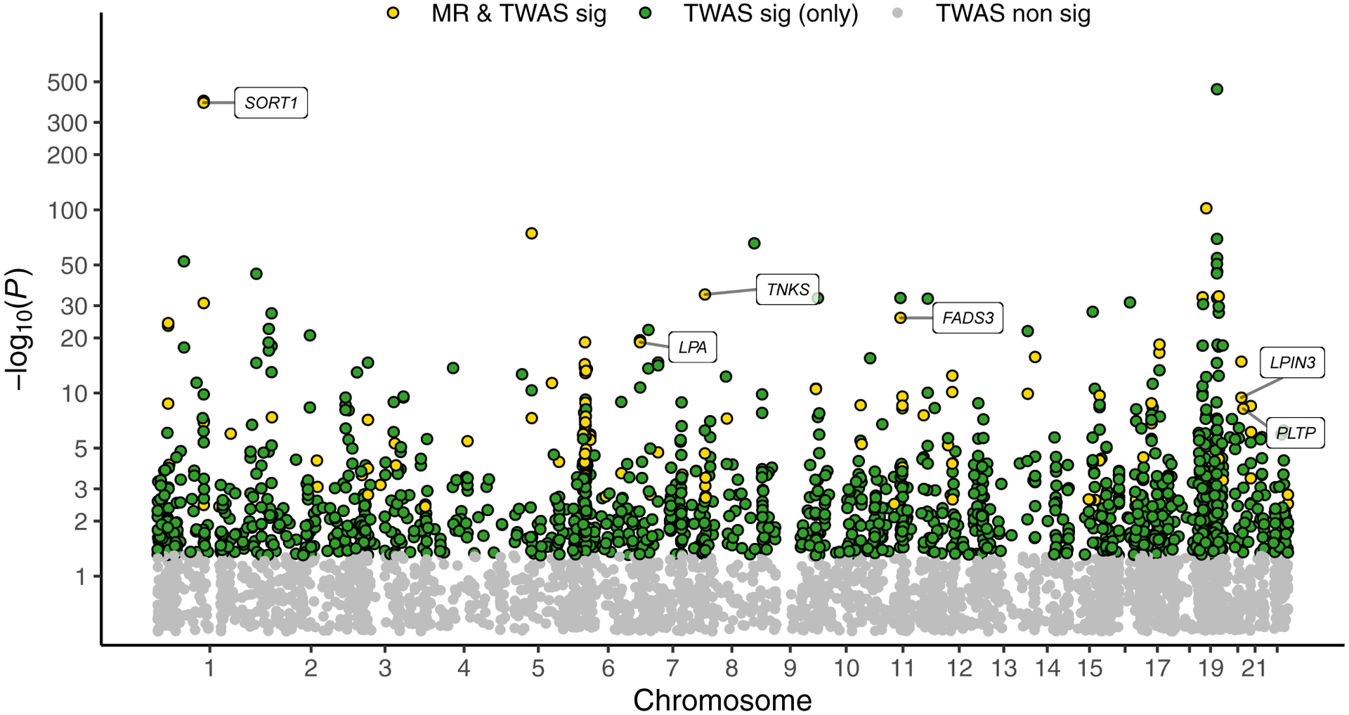
We performed causal inference using MR-JTI. The JTI results are highlighted on the TWAS Manhattan plot. Yellow, green, and grey dots denote the genes with both JTI and MR-JTI significance, only JTI significance, and non-JTI significance, respectively. In total, 138 genes had causal support for effect (Bonferroni-adjusted 95% confidence intervals do not contain 0) on LDL-C after heterogeneity control. Among the 138 genes, 6 are well-known LDL-C related genes. Additional results from the MR-JTI analysis are found in Supplementary Table 8.

To further investigate the performance of MR-JTI, we conducted MR analysis using MR-Egger, MR-PRESSO, SMR-HEIDI, and weighed median. MR-JTI outperformed the other methods, identifying more significant results (138) than the second best-approach, the weighted median (115). In addition, MR-JTI identified six genes from the literature-based silver standard (Methods), which is greater than the other approaches (Supplementary Table 9). Notably, we found that the 138 genes were significantly enriched for genes in the silver standard gene list (P < 0.001, the overlap [6] is 13.3 times as much as the expected count [0.45]) and, separately, in a conserved “cholesterol biosynthetic process” module in mice (P = 0.013, the overlap [16] is 1.68 times as much as the expected count [9.53])²⁵ (Supplementary Note). This analysis provides additional support for 16 of the MR-JTI significant genes (including PLTP, FASD3, and POLK, labeled in Supplementary Table 8 and 9).

DISCUSSION

By leveraging tissue similarity of gene expression and of epigenomic regulatory elements, our methodology significantly improved prediction accuracy especially in brain (which saw twice as many imputable genes) and other tissues with limited sample size. The improved imputation quality, in turn, increased the power for transcriptome-wide association.

We integrated DHS similarity across tissues in the weights used in the JTI loss function, exploiting the wide availability of DHS data. Further improvement can be expected from integrating other epigenomic datasets, including ATAC-seq, Hi-C, and histone modification ChIP-seq.

To evaluate the prediction performance, we applied the models to external data. Leveraging PsychENCODE, JTI resulted in almost double the number of iGenes, substantially outperforming UTMOST; leveraging GEUVADIS, JTI did not see as much improvement likely due to the smaller sample size of the reference panel and the high tissue-specificity of gene expression and DHS profile in LCLs. JTI identified more than 90% of the PrediXcan-derived iGenes, showing the flexibility of our framework, i.e. for tissues that have a highly tissue-specific profile, JTI automatically reduces to PrediXcan via hyper-parameter tuning.

The substantial performance gain for JTI relative to UTMOST may be attributable to several factors. Firstly, tissue similarity based on shared regulatory elements contains relevant information. Secondly, in contrast to UTMOST, JTI estimates only one effect size (not a different effect size) for each SNP across similar tissues. Thirdly, the flexible input window size for JTI captures much of the causal cis-regulatory information with reduced noise. Most multi-tissue eQTLs are closer to the gene body^26,27. Fourthly, in general, the genetic architecture of gene expression may have a better fit with JTI’s model (i.e., a middle ground between a sparse and polygenic architecture).

Applied to the LDL-C GWAS data, JTI showed consistent effect with PrediXcan for the top hits and detects additional associations for genes that were not well-imputed by PrediXcan. Indeed, a considerable number of gene-level associations were identified only by JTI. Among these genes, some were expected (including PPARG, KPNB1, PCSK9) while some were novel (e.g., POLK, TIRAP).

Horizontal pleiotropy is a primary challenge for MR-based studies, especially for a gene-based MR. LD contamination – the scenario in which (certain) SNP predictors for the gene under test are in LD with variants with an effect on the trait through a different causal gene in a GWAS locus – is an instance of horizontal pleiotropy (Extended Data Fig. 1). In our study, we developed a unified framework for TWAS and MR, with MR-JTI providing not only an imputation and association methodology (as PrediXcan has done), but also a causal inference framework (which was absent from PrediXcan). Due to widespread pleiotropy²⁸, we built a flexible framework to model the heterogeneity, with an approximately unbiased causal effect estimate. Aside from population stratification, which should have reduced effect in our ancestrally-homogeneous samples, the instruments should be independent (due to random assortment of genetic variation at gamete formation) of unmeasured confounders typically present in observational epidemiological studies which arise after conception. Any inflation may reflect the residual influence of weak instrument bias or horizontal pleiotropy due to invalid instruments. The enrichment of MR-JTI significant genes in the literature-based silver standard and, separately, in the conserved cholesterol modules in mice is further evidence that using MR-JTI for prioritization considerably increases the likelihood of capturing true causal genes.

MR-JTI differs fundamentally from FOCUS²⁹ and other approaches to causal inference. Both MR-JTI and FOCUS seek to prioritize genes based on the evidence for causality. FOCUS extends probabilistic SNP fine-mapping approaches, modeling the correlation among TWAS signals, to obtain credible gene sets containing the causal gene at a given confidence level. In contrast, MR-JTI aims to test for nonzero direct effect of the gene on the trait and to model instrumental-variable-level heterogeneity (mainly involving horizontal pleiotropy). Furthermore, MR-JTI differs from colocalization approaches³⁰, which aim to show that the same genetic instruments are causal for expression and for the trait. For a gene expression phenotype to be causal for a trait, having shared causal variants is necessary, but not sufficient.

JTI’s current implementation has some limitations. For some GTEx tissues, there is not a matched cell type with ENCODE or Roadmap DHS dataset. We could expect further improvement with more suitable cell types that capture the shared regulatory elements. Furthermore, shared samples across tissues were used to perform the training. Nevertheless, performance evaluation of JTI prediction in external datasets showed reliable prediction quality estimates, and extensive simulations demonstrated the type I error from the association was well-controlled. Finally, JTI had a higher replication rate than PrediXcan, indicating robust associations among the discovered genes.

In conclusion, we have developed a methodology with substantially improved statistical power for post-GWAS analysis. In principle, the approach offers an integrative framework for incorporating the vast functional genomic datasets that are being generated by genomic consortia to functionally annotate the genome. Finally, we implemented a broadly useful causal inference engine, leveraging the MR framework, to help prioritize the discovered genes for functional follow-up studies.

METHODS

Tissue-specific gene expression model building

PrediXcan performs gene expression imputation within a tissue using Elastic Net regularization, as previously described¹. Let y₁, y₂, …, y_n be the gene expression level in a given tissue for the n samples. A PrediXcan gene model solves the following minimization problem:

$$\widehat{\beta }=\text{arg}{\text{min}}_{\beta }\left(1/2\right){{\sum }_{i=1}^n\left(y_i-x_i^T\beta \right)}^2+\lambda \left(\left(\frac{1-\alpha }{2}\right){\Vert \beta \Vert }_2^2+\alpha {\Vert \beta \Vert }_1\right)$$ (1)

The L₁ penalty for the effect-size vector β induces sparsity while the L₂ penalty promotes grouping effect. The parameter α gives the relative weight of the two penalties; here we used α = 0.50. Equation (1) has a Bayesian formulation; solving the minimization problem is equivalent to determining the marginal posterior mode of β | y,λ₁,λ₂ assuming the following choice of prior distribution for β:

$$P\left(\beta \right)\alpha \text{exp}\left(-{\lambda }_2{\Vert \beta \Vert }_2^2-{\lambda }_1{\Vert \beta \Vert }_1\right)$$

which is a “combination” of Gaussian and Laplacian priors.

In this study, gene models were trained in the GTEx^7,8,20 v8 data in 49 tissues. The gene expression level used for training and testing was the residual of the normalized expression level after adjusting for covariates: gender, platform, first five principal components, and PEER factors for each tissue²⁰. Biallelic SNPs within 1 Mb of the gene were used as features. We included SNPs with minor allele frequency (MAF) > 0.05 and in Hardy-Weinberg equilibrium (P > 0.05). LD pruning was performed for SNPs at the r² = 0.9 level. (No significant difference in prediction quality was observed³¹.)

Building multi-tissue gene expression prediction models

We developed an alternative imputation approach, JTI, which borrows information across tissue transcriptomes. The approach leverages information from the other tissues in a tissue-dependent manner. Furthermore, JTI implements a novel approach to integrating high-throughput functional genomic data (such as from reference epigenomes generated by ENCODE³² and Roadmap³³) to improve prediction.

Let y = (y₁, y₂, …, y_n) be n observations. In our case, each observation is a tissue-sample pair. Let X = (x₁, x₂, … x_n)^T be the n × p feature matrix, where p is the number of features (genetic variants) for a gene expression model. Let β_true = (β_{1 true}, β_{2 true}, … β_{p true})^T be the effect-size vector for the p features. We estimate the effect-size vector β_true by solving the following optimization problem over all β:

$$\widehat{\beta }=\text{arg}{\text{min}}_{\beta }\left(1/2\right){\sum }_{i=1}^n{w}_i{\left(y_i-x_i^T\beta \right)}^2+\lambda \left(\left(\frac{1-\alpha }{2}\right){\Vert \beta \Vert }_2^2+\alpha {\Vert \beta \Vert }_1\right)$$ (2)

Here ‖β‖₂ and ‖β‖₁ are the L₂ and L₁ norm for β, respectively. The weight w_i on the i-th observation comes from the similarity matrix generated from the tuned hyper-parameters (see below). The weights are normalized to add up to the number of observations n through a scaling factor: $w_i=w_{i,old}\left(\raisebox{1ex}{$n$}\!\left/ \!\raisebox{-1ex}{${\sum }_{j=1}^n{w}_{j,old}$}\right.\right)$.

This model differs from the tissue-specific model (PrediXcan; equation [1]) in applying weights on tissue-sample pairs. Note the form of the penalty term, a combination of LASSO and ridge penalties, remains the same as in equation (1): $R\left(\beta \right)=\left(\frac{1-\alpha }{2}\right){\Vert \beta \Vert }_2^2+\alpha {\Vert \beta \Vert }_1$, as we want the gene expression model under JTI to continue to maintain the balance between sparsity and grouping effect for the features. The loss function L(y, f(x,β)) now incorporates the weight (see below for definition). Equation (2) has a natural Bayesian formulation that is equivalent to the log of the following likelihood:

$$P\left(\text{y}|\text{X},\beta \right)\alpha {\prod }_{i=1}^n{e}^{-L\left(y_i,f\left(x_i,\beta \right)\right)}$$

and the following choice of prior for β:

$$P\left(\beta \right)\alpha \text{exp}\left(-\lambda R\left(\beta \right)\right)$$

The estimated model $\widehat{\beta }$ (from equation [2]) is therefore equivalent to maximizing the conditional probability P(β | y), i.e., finding the posterior mode. In our current implementation, the penalty hyper-parameter λ was obtained from cross-validation and fixed. We performed external validation and extensive simulations to evaluate the performance of the model (Supplementary Note) in prediction and association analysis given the potential influence of non-linear effects and the shared samples across tissues.

As in the single-tissue PrediXcan models, JTI models were trained using the same data from the GTEx^7,8,20 v8 release. JTI used a flexible cis window size for model training. Since (1) most eQTLs (especially cross-tissue) tend to be close to the transcription start site (TSS)^8,26 and (2) a smaller window size will have less LD contamination (one of the major challenges of traditional TWAS with its lack of control for horizontal pleiotropy)³⁴, for each gene, the cis window size was determined based on cross-validation performance.

Incorporating regulatory elements

Cell-type specific DNase I hypersensitive sites (DHS), representing chromatin accessibility and potential trans-acting factor occupancy, were used as markers of regulatory regions. Some of the tissues in GTEx were mapped to the same cell type in ENCODE/Roadmap because of the lack of cell-type-specific data (Supplementary Table 10). Wig format DHS peaks were downloaded for each tissue/cell type, and quantile normalization was performed across each cell type. For each gene, the cis DHS similarity (in the region 10kb upstream and downstream of TSS) between the focal tissue and the other tissues was estimated by a monotonic function-based Spearman correlation (using “similaRpeak”³⁵).

Similarity matrix

One approach to defining the weights (w_i) in equation (2) is to set them to a constant, thereby weighing all tissue-sample pairs equally in the loss function. However, borrowing information across tissues may substantially improve prediction performance relative to the tissue-specific models.

For each tissue and gene pair, we considered the quantile-normalized gene-level DHS profile D (for a cell type that maps to the tissue) across the local region and the median gene expression level E (in the tissue) across the individuals. For a pair of tissues s and t, we calculated the correlation r_D in DHS profile D (gene-level similarity) and the correlation r_E in median gene expression E across the genes in the genome (tissue-level similarity) between the tissues. We assumed that the similarity between the two tissues is a (sufficiently) smooth function S(s, t) = f(r_D, r_E) of the correlations r_D and r_E. (More generally, this function can be generalized to be defined on an n-dimensional vector of correlations, such as from additional epigenome data.) One can therefore define S(s, t) as the Taylor expansion in (r_D, r_E) around (0, 0):

$$\text{S}\left(\text{s},\text{t}\right)={\sum }_{i,j}{a}_{ij}{r}_D{}^i{r}_E{}^j.$$

If the DHS profile and gene expression level are perfectly correlated between the two tissues (i.e., r_D = r_E = 1), we would define the two tissues to be perfectly correlated, which would impose the constraint ∑_i,ja_ij = 1. For computational tractability, we assumed that this similarity is driven by the leading monomial r_D^mr_Eⁿ. Note that in the simple case of the similarity matrix being equal to the identity matrix:

$$\text{S}\left(\text{s},\text{t}\right)=\{\begin{array}{c}1,s=t\\ 0,s\ne t\end{array}$$

i.e., where observations or tissue-sample pairs from a different tissue are given weight zero while observations in the test tissue are given weight one, then the loss function in equation (2) is the squared error for standard EN and consequently, JTI reduces to single-tissue PrediXcan as a special case.

In contrast to other methodologies⁵, our approach assigns a weight (w_i) to each observation i using relevant information on transcriptional regulation. For a given target tissue s, observations, i.e., tissue-sample pairs, from a tissue t with similar profiles on transcriptional regulation to the target tissue s are given higher weights.

Tuning hyper-parameters using grid search

We conducted hyper-parameter optimization on the similarity matrix using grid search. The choice of values for the hyper-parameter pair (m,n) may vary with tissue and gene, allowing borrowing of information from the other tissues in a gene- and tissue- dependent manner. The values for m and n were from the fixed space:

$$\Omega =\left\{\left(m,n\right)\in \mathbb{Z}\times \mathbb{Z}|m,n\in \left(4^0,4^1,4^2\dots ,4^L\right)\right\}$$

(In our analysis, L = 3.) In general, one can use any compact subset Ω of $\mathbb{Z}\times \mathbb{Z}$; however, the diameter of the lattice Ω determines the computational demands of the grid search. For each gene, five-fold cross-validation was performed for each pair (m,n). The pair with the minimal tuning error was chosen as the optimal pair.

S(s, t) in log-scale is a weighted sum of the correlations, where the weights are given by the hyper-parameters. Thus, the grid search attempts to find the nearly optimal combination of weights for the concordance measures from the input data (in this case, expression and DHS). Furthermore, single-tissue PrediXcan is a special instance of JTI, with the similarity matrix given by the identity matrix. This similarity matrix is equivalent to a specific choice of hyper-parameters (“at infinity”), i.e., PrediXcan and JTI are equivalent at m= n= ∞. This choice would be expected to perform well for genes with highly tissue-specific genetic regulation or expression profile (and which requires no leveraging of the similarity with any of the remaining tissues). As the hyper-parameter pair values – obtained from cross-validation – move away from infinity, JTI incorporates the similarity information in order to improve the prediction performance for the tissue under test.

Prediction performance

For each gene, we performed five-fold cross-validation for each tissue. The model performance was estimated using the correlation between the prediction $\widehat{{\text{y}}_{\mathit{\text{test}}}}=X_{\mathit{\text{test}}}\widehat{\beta }$ and the actual data y. A gene with $r=\text{corr}\left(y,\widehat{{\text{y}}_{\mathit{\text{test}}}}\right)>0.1$ and P < 0.05 was considered an imputable gene (iGene). The threshold r > 0.1 was justified based on simulations (Supplementary Fig. 3) and the testing performance in an external dataset (Supplementary Fig. 4). Genes that satisfied the loose threshold P < 0.05 from the imputation performance were kept so as not to severely limit the number of genes for the downstream association analysis.

Compared to the single-tissue prediction model, the gain in imputation performance (Δr²) and the increased proportion of imputable genes (ΔpiG) were plotted as functions of tissue sample size (N). To assess the impact of tissue sample size on model performance, we also built PrediXcan and JTI models using GTEx v6p data.

Comparison with existing methodologies

For comparison with other methodologies, we utilized 415 brain prefrontal cortex samples from PsychENCODE and 421 LCL samples from GEUVADIS³⁷ as external test data. To quantify the gain in prediction performance from leveraging the cross-tissue information, we ran several single-tissue approaches: the single-SNP “top eQTL” method and two multi-variant Bayesian approaches (performing 5-fold cross validation), namely, Bayesian Sparse Linear Mixed Model (BSLMM) using FUSION with default parameters³ and Dirichlet Process Regression (DPR)¹⁹, a nonparametric method with a Dirichlet process prior on effect-size variance, using ‘TIGAR’¹⁹.

We compared the prediction performance of JTI and UTMOST in the external datasets. However, the original UTMOST code may artificially inflate the prediction quality (Supplementary Note). We modified UTMOST by using uniform hyper-parameter pairs, which resolved the inflation (Supplementary Note). Compared to the performance in the external data, the cross-validation performance of the original UTMOST showed substantial inflation (Extended Data Fig. 6c). Our modification facilitated comparison of UTMOST with PrediXcan and JTI (Extended Data Fig. 6 and Extended Data Fig. 7).

Application to GWAS: discovery and replication

We developed JTI and PrediXcan²⁷ models using the GTEx v8 transcriptome data in 49 tissues and applied the models to GWAS data (Supplementary Table 1 and Supplementary Table 8 for sample sizes). For each GWAS sample, we estimated the genetically determined component $\widehat{{\text{y}}_{\mathit{\text{GWAS}}}}$ using X_GWAS,g, the genotype matrix of the contributing variants to the imputation model for the gene g:

$$\widehat{{\text{y}}_{\mathit{\text{GWAS}}}}=X_{\mathit{\text{GWAS}},g}\widehat{\beta }$$ (3)

The posterior predictive distribution of $\widehat{{\text{y}}_{\mathit{\text{GWAS}}}}$ given the observations y_reference from the reference panel allows one to estimate the uncertainty:

$$P\left(\widehat{{\text{y}}_{new}}|y_{\mathit{\text{reference}}}\right)=\int P\left(\widehat{{\text{y}}_{new}}|\beta ,y_{\mathit{\text{reference}}}\right)P\left(\beta |y_{\mathit{\text{reference}}}\right)\text{d}\beta$$

For primary illustration, we focus on the quantile-transformed LDL-C GWAS summary statistic data from UK biobank (released by Ben Neale Lab on 08/08/2019, http://www.nealelab.is/uk-biobank/). PrediXcan and JTI models for liver tissue were applied to summary-statistics. The SNP-SNP covariance matrices were estimated in the GTEx v8 samples. Replication was conducted in both the Global Lipids Genetics Consortium (GLGC) GWAS summary statistics (95,454 samples)³⁷ and the BioVU repository (18,394 European ancestry samples)³⁸.

In addition, we compared the association results of JTI and PrediXcan for additional traits, including HDL-C, glucose, schizophrenia (SCZ), bipolar disorder (BIP), Vitamin D, C-reactive protein, and rheumatoid factor (Supplementary Table 7).

Causal effect inference and the calculus of MR-JTI

MR-JTI performs multiple-instrumental-variable causal effect inference (Fig. 1) using summary data. The primary aim is to identify genes with causal effects on the trait of interest. However, the estimate of the causal effect of a gene on the trait, using the imputed expression – a weighted allele score – as a single instrumental variable, may be biased given invalid instruments in the allele score. If all instrumental variables are valid, then the estimated causal effect ($\widehat{\alpha }$) from JTI is unbiased, and JTI (without heterogeneity control) and Mendelian Randomization coincide. In our model-based approach, we estimate the contribution of each genetic instrument to the overall heterogeneity given the possibility of invalid instruments¹⁶. Under the Instrument Strength Independent of Direct Effect (InSIDE) assumption, this approach yields a consistent estimate of the causal effect.

For causal inference of the gene-level effect on a trait, we must obtain an unbiased estimate in the presence of invalid instruments. PrediXcan provided an association test but did not attempt to control heterogeneity. Consider J independent genetic instrumental variables x₁, x_2, …, x_J to test for the effect of the gene g on the phenotype y. For the j-th variant, let β_j and θ_j be its effect size on gene expression and on the phenotype, respectively, from summary statistics on genetic associations. For a causal gene on the phenotype, the relationship between the instrumental variable x_j and g and the relationship between x_j and y, for all J valid instrumental variables, are given by the following model:

$$E\left(g|{\text{x}}_j=x\right)={\text{a}}_j+{\beta }_{j}x$$

$$E\left(y|{\text{x}}_j=x\right)={\text{b}}_j+{\theta }_{j}x$$

The relationship between the gene expression trait g and y is given by:

$$E\left(y|g\right)=c+\alpha g$$

Here α encodes the (nonzero) direct effect of the gene on the trait; a_j and b_j are scalars that may vary with the instrumental variable; and c is an intercept term (i.e., the value of the trait when gene expression is zero) for the gene-phenotype relationship. Assuming that these linear relationships hold and that each x_j is a valid instrumental variable, then a direct causal effect of g on y (i.e., $\frac{\partial y}{\partial g}\ne 0$) is equivalent to the “chain rule” (with a nonzero instrumental-variable effect on y, i.e., $\mathit{\theta }\ne \overrightarrow{0}$, only through g):

$${\theta }_i=\frac{\partial y}{\partial x_i}=\frac{\partial y}{\partial g}\frac{\partial g}{\partial x_i}={\alpha \beta }_i$$

or

$$\mathit{\theta }=\mathit{\nabla }\mathit{y}=\left(\frac{\partial y}{\partial g}\right)\mathit{\nabla }\mathit{g}=\alpha \mathit{\beta }$$

where ∇ is the gradient operator. We note that the middle equality does not require ∇y and ∇g to be constant (that is, y and g to be linear in the instrumental variables), and causal inference can be performed in a more general context. Here, the partial-derivative operator $\frac{\partial }{\partial x_i}$ applied to a function f (e.g., y or g) is defined as follows:

$$\frac{\partial f}{\partial x_i}\left(x\right):=\underset{\vartheta \to 0}{\text{lim}}\raisebox{1ex}{$\left(E\left[f|x_i=x+\vartheta \right]-E\left[f|x_i=x\right]\right)$}\!\left/ \!\raisebox{-1ex}{$\vartheta $}\right.$$

Marginal relevance (∇g ≠ 0), confounder independence ($\frac{\partial U}{\partial x_i}=0$, for each confounder U and each instrumental variable x_i), and exclusion restriction (i.e., $\frac{\partial y}{\partial g_{*}}$ exists only for g_* = g) are encoded in the relationship. Let us suppose that there are additional causal pathways g_*,k by which the instrumental variables influence the phenotype y, resulting in a violation of exclusion restriction; that is, $\frac{\partial y}{\partial g_{*,k}}\ne 0$ for each k. Then, the generalized chain rule yields:

$$\mathit{\theta }=\alpha \mathit{\beta }+\sum _k\left(\frac{\partial y}{\partial g_{*,k}}\right)\mathit{\nabla }{\mathit{g}}_{*,\mathit{k}}$$

In this case, a nonzero β (from the assumption of marginal relevance) and a nonzero θ (from the association of the same instruments with the trait) do not necessarily imply a causal effect of the test gene g on the trait (i.e., α ≠ 0).

Here, we model the heterogeneity

$$\mathit{h}:=\mathit{\theta }-\alpha \mathit{\beta }=\sum _k\left(\frac{\partial y}{\partial g_{*,k}}\right)\mathit{\nabla }{\mathit{g}}_{*,\mathit{k}}$$

as a linear sum of the contribution of independent instrumental variables since (a) horizontal pleiotropy (i.e., the existence of a causal pathway due to g_*,k distinct from the test gene g) can be widespread, (b) whether an instrumental variable is valid is not a priori known in most cases (so that ruling out horizontal pleiotropy g_*,k is not easily verifiable and the corresponding effect, i.e., $\frac{\partial y}{\partial g_{*,k}}$ with ∇g_*,k ≠ 0, must be inferred), and (c) weak instrument bias (a form of finite sample bias in the estimate of ∇g or β) may cause departure from asymptotics. The heterogeneity h is the aggregate effect of all PSB. We then perform parameter estimation:

$$\widehat{h}=\widehat{\mathit{\theta }}-\widehat{\alpha }\widehat{\mathit{\beta }}={\sum }_{k=1}^J\widehat{{\delta }_k}{\mathit{e}}_{\mathit{k}}+\widehat{\omega }l$$ (4)

where $\widehat{\mathit{\theta }}\stackrel{\text{def}}{=}\left[\widehat{{\theta }_j}\right]$ and $\widehat{\mathit{\beta }}\stackrel{\text{def}}{=}\left[\widehat{{\beta }_j}\right]$ are J-dimensional vectors with entries given by the estimated effects on trait and gene expression, respectively, of the instrumental variables (from GWAS and the eQTL data, respectively), e_k is the unit vector with 1 in the k-th position and 0 elsewhere, and $\mathit{l}\stackrel{\text{def}}{=}\left[{\text{l}}_j\right]$ is the vector of LD-score for all the variants with its estimated effect $\widehat{\omega }$. Note that in this model, when all instrumental variables are valid, then δ_j = 0, for all j and ω = 0.

An alternative approach is to model h, with each component a random effect. In particular,

$$\widehat{\mathit{\theta }}~\mathit{N}\left(\alpha \mathit{\beta },{\sigma }_{\theta }^{2}I\right)$$

$$\widehat{\mathit{\beta }}~\mathit{N}\left(\mathit{\beta },{\sigma }_{\beta }^{2}I\right)$$

$$\widehat{\mathit{h}}=\widehat{\mathit{\theta }}-\widehat{\alpha }\widehat{\mathit{\beta }}~\mathit{N}\left(\overrightarrow{0},{\phi }^{2}I\right)$$

where ${\phi }^2={\sigma }_{\theta }^2+{\widehat{\alpha }}^2{\sigma }_{\beta }^2$ and ${\sigma }_{\theta }^2$ is upward-biased by horizontal pleiotropy. We obtained an expression for the log likelihood of the GWAS and eQTL effect size data (assuming the independence of the datasets):

$$\text{log}L=-\frac{1}{2}\left[\sum _{i=1}^J\frac{{\left(\widehat{{\beta }_i}-{\beta }_i\right)}^2}{{\sigma }_{\beta }^2}+\sum _{i=1}^J\frac{{\left(\widehat{{\theta }_i}-\alpha {\beta }_i\right)}^2}{{\sigma }_{\theta }^2}\right]-\frac{J}{2}\text{log}\left(4{\pi }^2{\sigma }_{\beta }^2{\sigma }_{\theta }^2\right)$$

We define an estimator for α as follows:

$${\widehat{\alpha }}_{*}=\underset{\alpha }{\text{argmax}}\left[\underset{\beta }{\text{sup}}\text{log}L\left(\mathit{\beta },\alpha \right)\right]=\underset{\alpha }{\text{argmax}}\text{log}L\left({\mathit{\beta }}_{*},\alpha \right)$$

Where β_* is a vector with i-th component given by:

$${\mathit{\beta }}_{*,i}=\frac{{\sigma }_{\theta }^2\widehat{{\beta }_i}+\alpha \widehat{{\theta }_i}{\sigma }_{\beta }^2}{{\sigma }_{\theta }^2+{\alpha }^2{\sigma }_{\beta }^2}$$

However, the estimator ${\widehat{\alpha }}_{*}$ is statistically inconsistent.

To detect heterogeneity (equation (4)), we are looking for deviation from this Wald ratio estimate.

$$\widehat{\alpha }=\frac{\widehat{{\theta }_j}}{\widehat{{\beta }_j}}$$ (5)

The length of the vector ${\sum }_{k=1}^J\widehat{{\delta }_k}{\mathit{e}}_k+\widehat{\omega }l$, which is the difference-vector between the GWAS-defined vector $\widehat{\mathit{\theta }}$ and the expression-defined vector $\widehat{\alpha }\widehat{\mathit{\beta }}$, provides an estimate of the overall heterogeneity. One can perform the following LASSO optimization problem to estimate the gene causal effect ($\widehat{\alpha }$), the contribution ($\widehat{{\delta }_j}$) of the j-th instrument to the heterogeneity, and the effect ($\widehat{\omega }$) of LD confounding:

$$\widehat{\alpha },\widehat{\delta ,}\widehat{\omega }=\underset{\text{u},v_j,\text{w}}{\text{argmin}}\sum _{j=1}^J{\left(\widehat{{\theta }_j}-u\widehat{{\beta }_j}-v_j-w{l}_j\right)}^2+\lambda \left({\Vert \left[v_j\right]\Vert }_1+\left|u\right|+\left|w\right|\right)$$

The optimization problem aims to minimize the objective function (the error in predicting the GWAS effect at a variant from the regulatory effect on expression, the causal effect of the gene on the trait, and the heterogeneity) while enforcing sparsity; that is, we estimate the heterogeneity through optimization in the search space, preferring a model with fewer predictors and about the same explanatory power. However, LASSO provides a weakly consistent estimator with a complicated asymptotic distribution³⁹. We sought to estimate the standard error for each of these estimates using the bootstrap. However, the bootstrap is inconsistent^40,41 in case one or more of the regression parameters is zero (e.g., in the presence of one more valid instrumental variable)^47,48. We define a modified LASSO estimator $\widehat{S}\stackrel{\text{def}}{=}\left({\widehat{\alpha }}_{*},{\widehat{\delta }}_{*},{\widehat{\omega }}_{*}\right)$ of the true value S.

$$\widehat{S}\stackrel{\text{def}}{=}\left({\widehat{\alpha }}_{*},{\widehat{\delta }}_{*},{\widehat{\omega }}_{*}\right)=\{\begin{array}{c}{\widehat{\alpha }}_{*},\widehat{{\delta }_{j,*},}{\widehat{\omega }}_{*}\text{if}\left|{\widehat{\alpha }}_{*}\right|,\widehat{|{\delta }_{j,*}}\left|,\right|{\widehat{\omega }}_{*}|\ge \frac{1}{J+2}\text{respectively}\\ 0\text{if}|{\widehat{\alpha }}_{*}\left|,\widehat{|{\delta }_{j,*}}\right|,\left|{\widehat{\omega }}_{*}\right|<\frac{1}{J+2}\text{respectively}\end{array}$$

We utilized a modified (threshold) residual bootstrap LASSO approach^40,41. This approach provides an estimator $\widehat{T_{m,**}}$ that has the property of being consistent, i.e.,

$$\underset{m\to \infty }{\text{plim}}\widehat{T_{m,**}}=S$$

That is, the estimator $\widehat{T_{m,**}}$ converges in probability to S, i.e., for any fixed τ > 0,

$$\underset{m\to \infty }{\text{lim}}\text{Pr}(|\widehat{T_{m,**}}-S|>\tau \text{)}=0$$

MR-JTI analysis of GWAS data

The genetic associations with exposure (eQTLs in the cis-region) and with the GWAS trait (QTLs) were analyzed in European-ancestry samples (thus reducing the possibility of confounding) in a two-sample Mendelian Randomization framework using summary statistics data. There is no sample overlap between the eQTL and GWAS datasets. Our approach leverages multiple genetic instruments, consistent with the observed allelic heterogeneity²⁰ in gene expression, and estimates the heterogeneity.

We harmonized genetic variants across the eQTL and GWAS datasets to ensure that the per additive copy of the same allele was used in the MR-JTI analysis, following the guidelines for MR investigations^42,43. In our study, the genotype resource for both the eQTL and the GWAS datasets were coded on the positive genomic strand. Only biallelic variants were included in the MR-JTI analysis. Allele and strand information were used to detect potential strand mismatch. In addition, palindromic variants with a MAF greater than 0.45 were removed since it would be nearly impossible to verify that the alleles had been correctly orientated⁴². LD pruning was performed using PLINK (--indep-pairwise 50 5 0.2) to decorrelate the SNPs in the cis-window.

A characteristic feature of our approach is the testing of genes in the human transcriptome as exposures, resulting in a large number of hypotheses. We defined Bonferroni-adjusted P < 0.05 as significant. Although this approach is conservative (and Mendelian Randomization may suffer from low power), we aim to identify potentially causal genes with the strongest support from an integrative GWAS-eQTL analysis.

Furthermore, although the estimated causal effect of the gene on the trait, as derived from Mendelian Randomization, must be interpreted with caution (as the MR guidelines have pointed out⁴²), our approach ultimately seeks to prioritize genes based on the presence of causal effect on the trait, providing a resource for further functional studies (e.g., CRISPR). We conducted analyses on a GWAS of LDL-C, using a literature-based silver standard (Supplementary Table 4), to compare MR-JTI and other MR approaches (see Supplementary Note).

Correlation among effect size estimates and Mendelian Randomization analysis

We evaluated the impact of the correlation among the GWAS effect size estimates ${\widehat{{\theta }_{\text{j}}}}^{\prime }\text{s}$ and, similarly, the correlation among the regulatory effect size estimates ${\widehat{{\beta }_{\text{j}}}}^{\prime }\text{s}$ on the analysis. Given effect size estimates $\widehat{{\theta }_{\text{j}}}$ and $\widehat{{\theta }_{\text{k}}}$ on the trait for the j-th and k-th instrument, respectively, the following relationship holds:

$$\text{corr}\left(\widehat{{\theta }_{\text{j}}},\widehat{{\theta }_{\text{k}}}\right)=2\sqrt{\raisebox{1ex}{$h_j^2{h}_k^2$}\!\left/ \!\raisebox{-1ex}{$\left(1-h_j^2\right)\left(1-h_k^2\right)$}\right.}$$

where $h_j^2$ and $h_k^2$ are the per-SNP contribution to trait variance (heritability) of the j-th and k-th instrument, respectively. For a highly polygenic trait, this quantity is small owing to the modest per-SNP contribution to the trait variance. For gene expression with allelic heterogeneity, the corresponding quantity $\text{corr}\left(\widehat{{\beta }_{\text{j}}},\widehat{{\beta }_{\text{k}}}\right)$ is small for a large proportion of genes (using the imputation quality from the training as an estimate of gene expression heritability). Thus, the pairwise correlations between these effect sizes are small, and the simple model θ = αβ (i.e., without the higher-order terms from the pairwise terms) is a good fit, as was also shown empirically by the recent study²⁰.

Statistical tests

All statistical tests are two-sided unless otherwise stated.

CODE AVAILABILITY

The code for JTI and MR-JTI and for reproducing the figures in this paper is available on github (https://github.com/gamazonlab/MR-JTI).

DATA AVAILABILITY

The protected data for the GTEx project (for example, genotype and RNA-sequence data) are available via access request to dbGaP accession number phs000424.v8.p2. Processed GTEx data (for example, gene expression and eQTLs) are available on the GTEx portal: https://gtexportal.org. The URLs of the summary statistics datasets of all the GWAS meta-analyses analyzed in the paper can be found in Supplementary Table 7. All summary results from the gene-based analyses are in Supplementary Tables. The JTI GTEx models (as well as the PrediXcan and [modified] UTMOST models we generated) are available for download on Zenodo (http://doi.org/10.5281/zenodo.3842289). The PsychENCODE (http://doi.org/10.5281/zenodo.3859065) and GEUVADIS (https://doi.org/10.5281/zenodo.3859075) models have also been deposited.

Extended Data

Extended Data Fig. 1. TWAS could be biased by possible sources of bias (PSB), including invalid instrumental variables (IVs) due to horizontal pleiotropy and weak instruments.

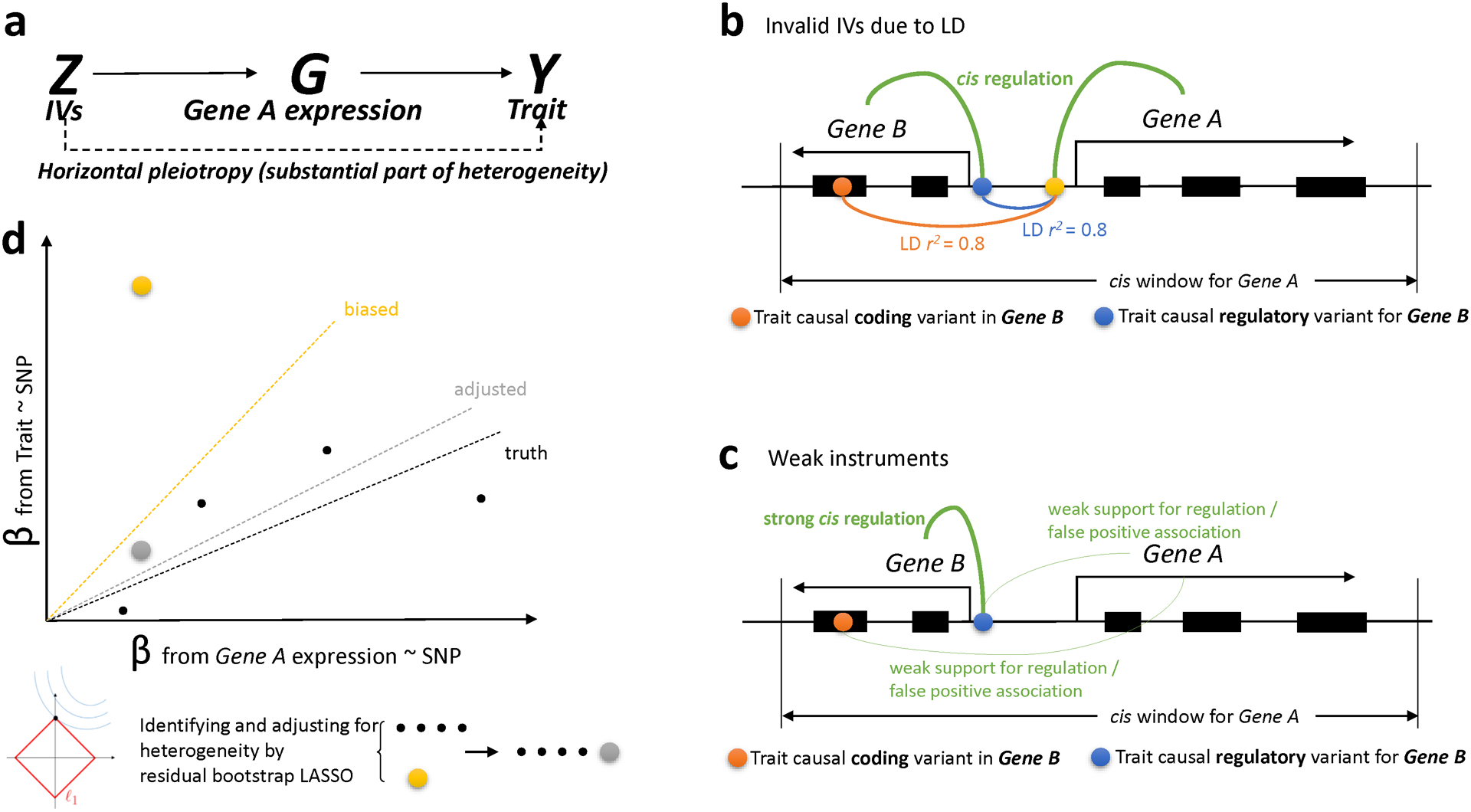
Conventional TWAS, such as PrediXcan, can be viewed as Mendelian Randomization with multiple IVs, but without horizontal pleiotropy control. a, A major source of false positives from TWAS is the use of invalid IVs due to horizontal pleiotropy. b, Horizontal pleiotropy can arise in multiple ways. For example, it can come from LD-induced invalid IVs, i.e., LD contamination. If we are testing the significance of Gene A, but one of the SNPs (yellow) in the prediction model tags another coding (red) or regulatory (blue) variant that is causal for the trait through another Gene B, causal effect estimation will be biased. c, Even without LD contamination, the estimation may also be biased by the inclusion of weak or false positive eQTLs in the prediction model for Gene A. In this case, the effect of the weak or false positive eQTL for Gene A on the trait is actually mediated by another Gene B (by affecting coding or regulation). More generally, weak instrument bias is a type of finite sample bias; it arises in finite samples where the gene expression (“exposure”) is only weakly correlated with the instrument set. Both b, and c, result in d, a biased estimate of gene causal effect on trait. We estimate the heterogeneity due to PSB using threshold-based residual bootstrap LASSO (see Methods). Our approach estimates the heterogeneity due to invalid IVs and gives an adjusted estimate of the gene causal effect on trait.

Extended Data Fig. 2. The gene expression similarity matrix.

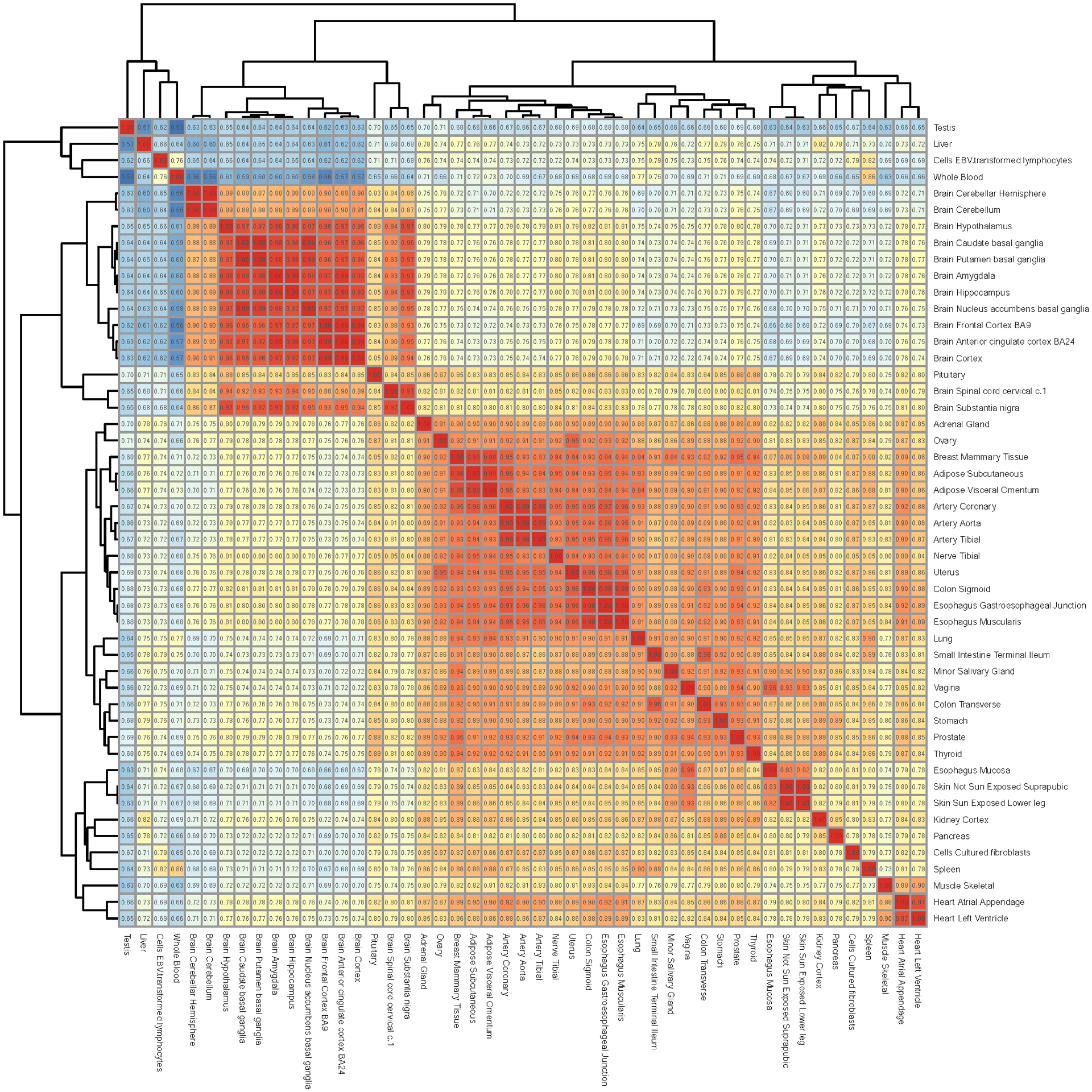
The median expression level (log₂-transformed TPM) across all the samples of a given tissue was used to evaluate the correlation (Pearson) of tissue-tissue pairs across the transcriptome. The similarity map was generated by performing hierarchical clustering.

Extended Data Fig. 3. Comparison of prediction performance between PrediXcan and JTI in all GTEx v8 tissues.

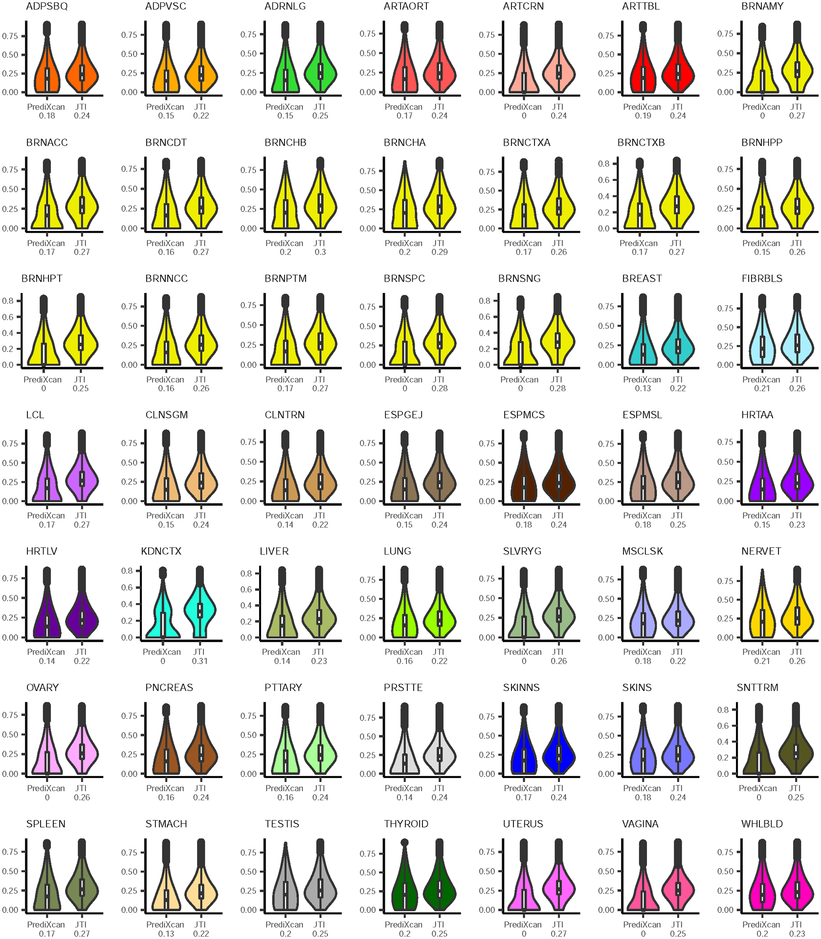
We compared the performance of PrediXcan and JTI using the Pearson correlation r between predicted and observed expression levels for each of the 49 GTEx v8 tissues with more than 70 samples. The white box edges depict interquartile range, whiskers 1.5× the interquartile range, center black dot marks the median level, and the outlines display the kernel probability density. The median correlation is also shown below the x-axis label.

Extended Data Fig. 4. Prediction performance comparison between JTI and three single-tissue approaches (top eQTL, BSLMM, and DPR) in two independent datasets.

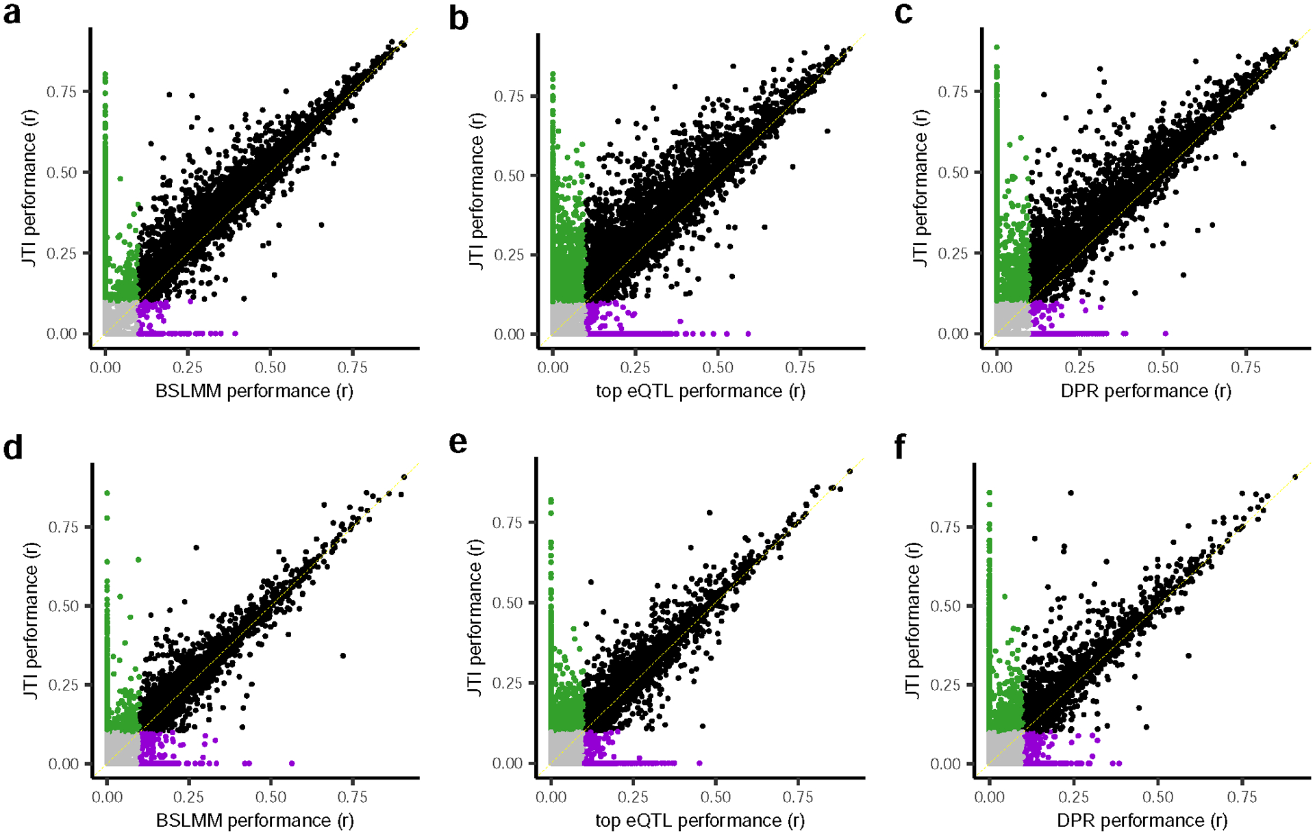
Prediction models were trained using BLSMM (5-fold cross-validation FUSION default setting) and JTI (see Methods) in GTEx v8 a, brain frontal cortex BA9 region and d, EBV-transformed lymphocytes. The x-axis and y-axis represent the Pearson correlation r between the predicted expression and observed expression in external (non-GTEx and independent) datasets. i.e., a, PsychENCODE and d, GEUVADIS. b, and e, show the corresponding comparisons between JTI and top eQTL, which simply models the genetically regulated expression using the top eQTL. c, and f, We also compared the prediction performance with the DPR model, a nonparametric Bayesian method with a Dirichlet process prior on effect-size variance, using the software tool ‘TIGAR’ with 5-fold cross-validation. The green, purple, and pink dots denote genes imputable using only JTI, BSLMM, top eQTL, and DPR, respectively. The black and grey dots denote genes consistently imputable and not imputable, respectively, using both methods.

Extended Data Fig. 5. JTI and PrediXcan showed a substantial increase in iGene discovery between GTEx v6p and v8.

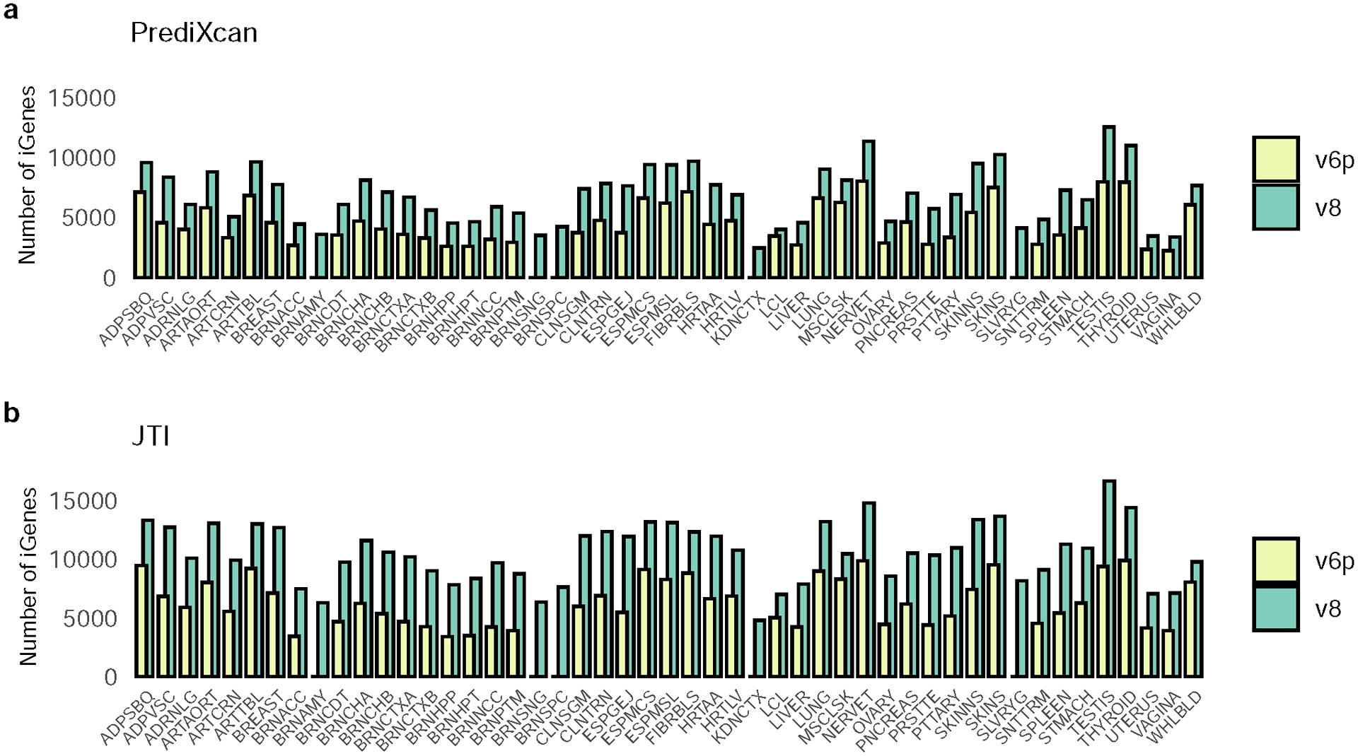
We compared the number of imputable genes across all the tissues between GTEx v6p (yellow) and v8 (green). The prediction performance of GTEx v8 was superior to v6p for both a, PrediXcan and b, JTI in all tissues. The number of iGenes can be found in Supplementary Table 1.

Extended Data Fig. 6. Prediction performance comparison among PrediXcan, JTI, original UTMOST, and modified UTMOST for brain frontal cortex BA9.

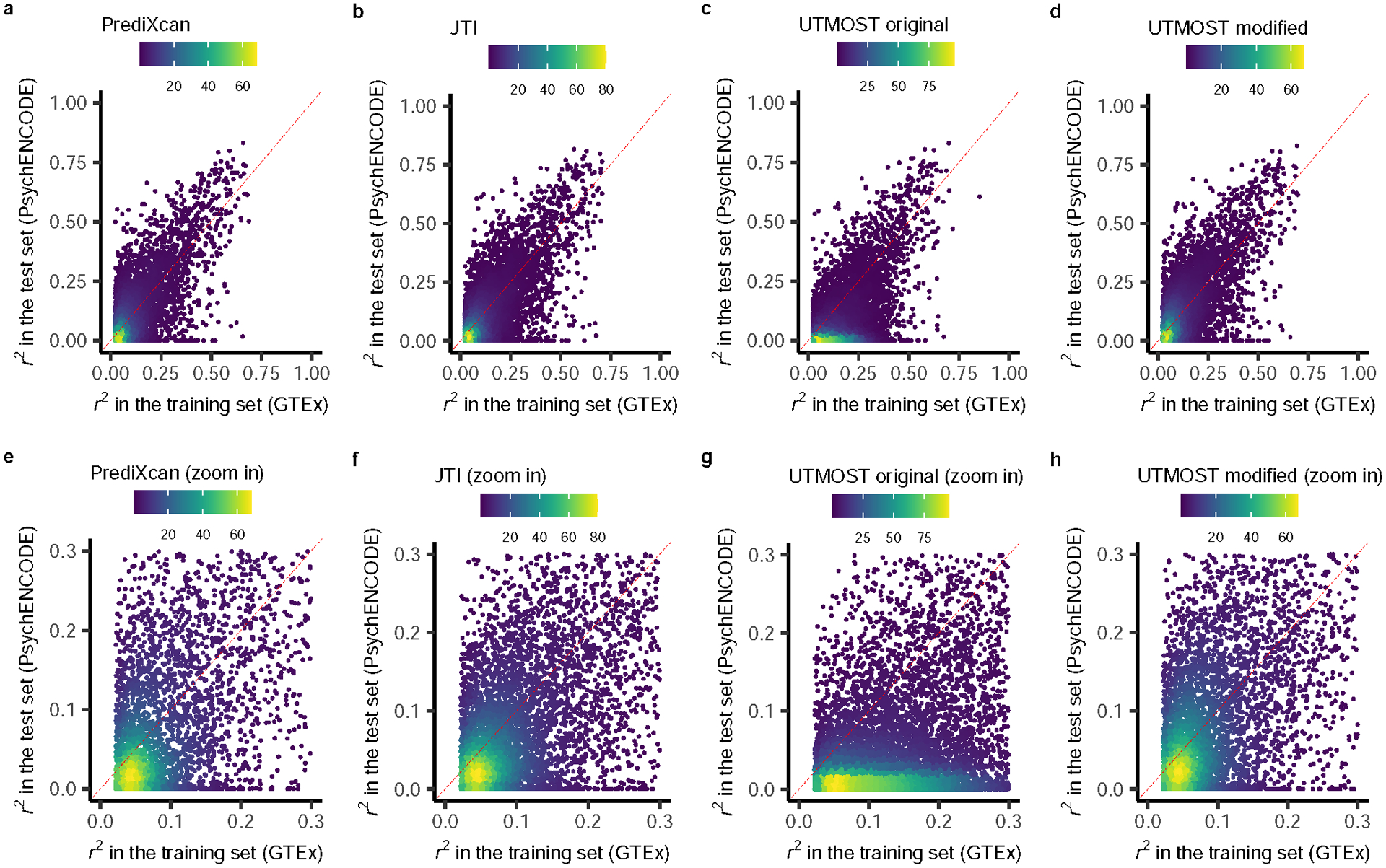
We compared the cross-validation prediction performance (r²) in GTEx (internal, brain frontal cortex BA9) and the prediction performance in PsychENCODE (an external test data set, brain prefrontal cortex) among a, PrediXcan, b, JTI, c, original UTMOST, and d, modified UTMOST. The lower figures e, f, g, and h, are the zoom-in version of the corresponding upper figures. The yellow, green, and purple dots indicate high, medium, and low density.

Extended Data Fig. 7. Prediction performance comparison among PrediXcan, JTI, original UTMOST, and modified UTMOST for EBV transformed lymphocytes.

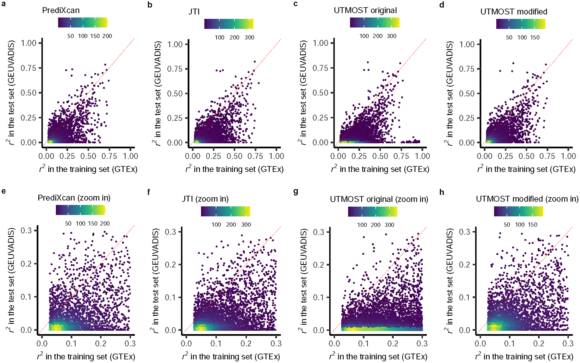
We compared the cross-validation prediction performance (r²) in GTEx (internal, EBV transformed lymphocytes) and the prediction performance in GEUVADIS (an external test data set, LCLs) among a, PrediXcan, b, JTI, c, original UTMOST, and d, modified UTMOST. The lower figures e, f, g, and h, are the zoom-in version of the corresponding upper figures. The yellow, green, and purple dots indicate high, medium, and low density.

Extended Data Fig. 8. Type I error rate for PrediXcan, UTMOST, and JTI.

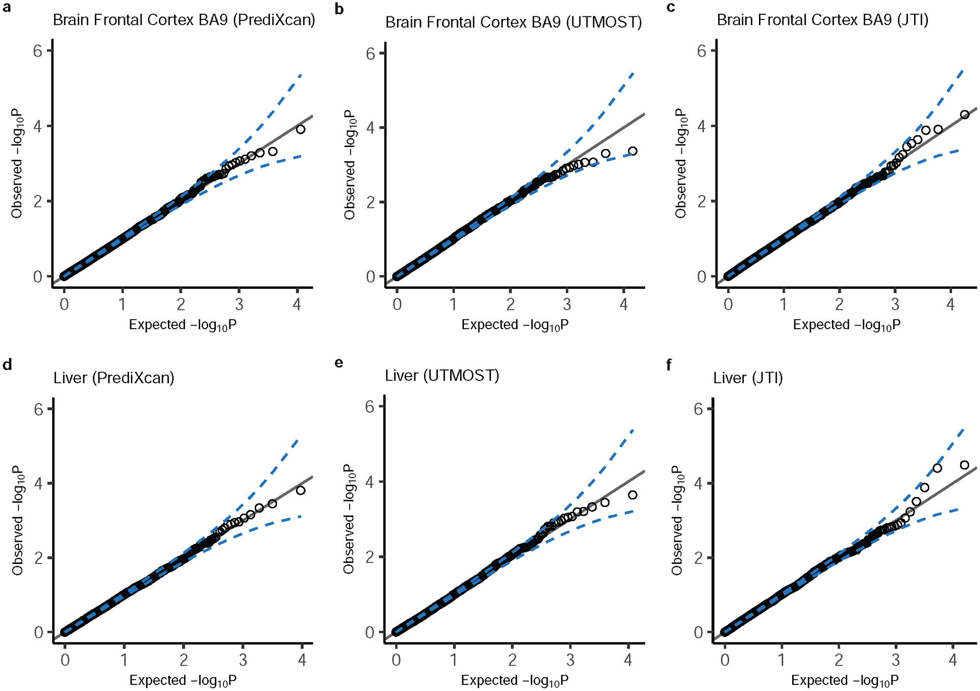
The Q-Q plots show the type I error from applying PrediXcan, UTMOST, and JTI models in a, b, and c brain frontal cortex BA9 and d, e, and f, Liver. The blue dashed lines show the 95% CI of the expected -log(P). Type I error rate for all the tissues can be found in Supplementary table 3.

Extended Data Fig. 9. TWAS power analysis for PrediXcan, UTMOST, and JTI.

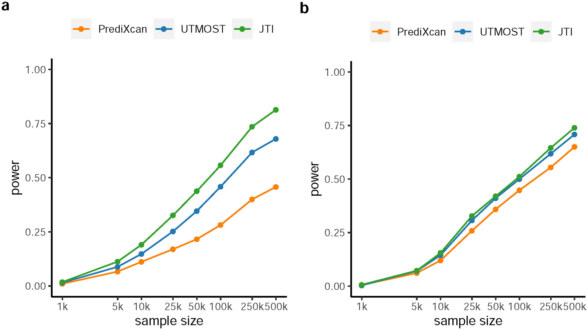
The true expression level of randomly sampled causal genes and the effect size for each gene on trait were simulated. In this model, each gene, on average, contributed 0.5% to the phenotypic variance. For each gene, the predicted (i.e., genetically determined) expression level was generated according to the proportion of variance explained (PVE), based on the actual prediction performance (R²) in two external datasets (a, PsychENCODE and b, GEUVADIS), for each of the three imputation approaches (PrediXcan, UTMOST, and JTI). Power was estimated as the proportion of simulations that attain significance (defined as Bonferroni adjusted P < 0.05).

Extended Data Fig. 10. Comparison of the estimated gene effect size on LDL-C from MR-JTI and the median estimator (median level of Wald ratio estimates across all cis-eQTLs).

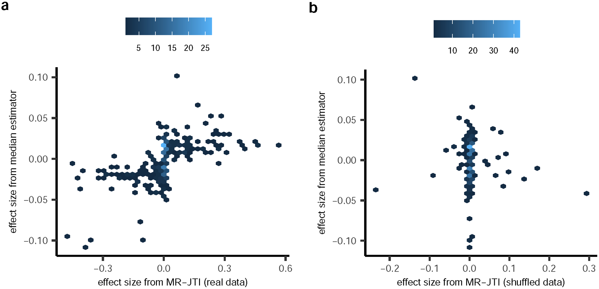
For each gene, the median estimator was calculated as the median of the Wald ratio estimates across all the cis-eQTLs. The Wald ratio estimate for a cis-eQTL is the ratio of the estimate for the GWAS effect size and the estimate for the eQTL effect size.

a, Positive correlation between the estimated gene effect size from MR-JTI and the median estimator effect size (Spearman r = 0.72, P < 2.2e-16) was observed. b, No significant correlation was observed between the median estimator and the MR-JTI estimate from shuffled GWAS summary statistics data. Furthermore, note that MR-JTI’s type I error is well-controlled.

REFERENCES

- 1.Gamazon ER et al. A gene-based association method for mapping traits using reference transcriptome data. Nat Genet 47, 1091–8 (2015). [DOI] [PMC free article] [PubMed] [Google Scholar]
- 2.Zhu Z et al. Integration of summary data from GWAS and eQTL studies predicts complex trait gene targets. Nature genetics 48, 481 (2016). [DOI] [PubMed] [Google Scholar]
- 3.Gusev A et al. Integrative approaches for large-scale transcriptome-wide association studies. Nature genetics 48, 245 (2016). [DOI] [PMC free article] [PubMed] [Google Scholar]
- 4.Barbeira AN et al. Integrating predicted transcriptome from multiple tissues improves association detection. PLoS genetics 15, e1007889 (2019). [DOI] [PMC free article] [PubMed] [Google Scholar]
- 5.Hu Y et al. A statistical framework for cross-tissue transcriptome-wide association analysis. Nature genetics 51, 568–576 (2019). [DOI] [PMC free article] [PubMed] [Google Scholar]
- 6.Flutre T, Wen X, Pritchard J & Stephens M A statistical framework for joint eQTL analysis in multiple tissues. PLoS genetics 9(2013). [DOI] [PMC free article] [PubMed] [Google Scholar]
- 7.Consortium GTEx. Human genomics. The Genotype-Tissue Expression (GTEx) pilot analysis: multitissue gene regulation in humans. Science 348, 648–60 (2015). [DOI] [PMC free article] [PubMed] [Google Scholar]
- 8.Consortium GTEx et al. Genetic effects on gene expression across human tissues. Nature 550, 204–213 (2017). [DOI] [PMC free article] [PubMed] [Google Scholar]
- 9.Urbut SM, Wang G, Carbonetto P & Stephens M Flexible statistical methods for estimating and testing effects in genomic studies with multiple conditions. Nature genetics 51, 187–195 (2019). [DOI] [PMC free article] [PubMed] [Google Scholar]
- 10.Aguet F et al. The GTEx Consortium atlas of genetic regulatory effects across human tissues. BioRxiv, 787903 (2019). [DOI] [PMC free article] [PubMed] [Google Scholar]
- 11.Pierce BL & Burgess S Efficient design for Mendelian randomization studies: subsample and 2-sample instrumental variable estimators. American journal of epidemiology 178, 1177–1184 (2013). [DOI] [PMC free article] [PubMed] [Google Scholar]
- 12.Burgess S & Thompson SG Use of allele scores as instrumental variables for Mendelian randomization. International Journal of Epidemiology 42, 1134–1144 (2013). [DOI] [PMC free article] [PubMed] [Google Scholar]
- 13.Smith GD & Ebrahim S Mendelian randomization: prospects, potentials, and limitations. International journal of epidemiology 33, 30–42 (2004). [DOI] [PubMed] [Google Scholar]
- 14.Johnson T Efficient calculation for multi-SNP genetic risk scores Technical Report, The Comprehensive R Archive Network. (2013). [Google Scholar]
- 15.Burgess S, Butterworth A & Thompson SG Mendelian randomization analysis with multiple genetic variants using summarized data. Genetic epidemiology 37, 658–665 (2013). [DOI] [PMC free article] [PubMed] [Google Scholar]
- 16.Bowden J, Davey Smith G & Burgess S Mendelian randomization with invalid instruments: effect estimation and bias detection through Egger regression. International journal of epidemiology 44, 512–525 (2015). [DOI] [PMC free article] [PubMed] [Google Scholar]
- 17.Bowden J, Davey Smith G, Haycock PC & Burgess S Consistent estimation in Mendelian randomization with some invalid instruments using a weighted median estimator. Genetic epidemiology 40, 304–314 (2016). [DOI] [PMC free article] [PubMed] [Google Scholar]
- 18.Verbanck M, Chen C. y., Neale B & Do R Detection of widespread horizontal pleiotropy in causal relationships inferred from Mendelian randomization between complex traits and diseases. Nature genetics 50, 693–698 (2018). [DOI] [PMC free article] [PubMed] [Google Scholar]
- 19.Nagpal S et al. Tigar: An improved bayesian tool for transcriptomic data imputation enhances gene mapping of complex traits. The American Journal of Human Genetics 105, 258–266 (2019). [DOI] [PMC free article] [PubMed] [Google Scholar]
- 20.Barbeira AN et al. Widespread dose-dependent effects of RNA expression and splicing on complex diseases and traits. BioRxiv, 814350 (2019). [Google Scholar]
- 21.Bavoux C, Hoffmann J & Cazaux C Adaptation to DNA damage and stimulation of genetic instability: the double-edged sword mammalian DNA polymerase κ. Biochimie 87, 637–646 (2005). [DOI] [PubMed] [Google Scholar]
- 22.Williams HL, Gottesman ME & Gautier J Replication-independent repair of DNA interstrand crosslinks. Molecular cell 47, 140–147 (2012). [DOI] [PMC free article] [PubMed] [Google Scholar]
- 23.Shimizu I, Yoshida Y, Suda M & Minamino T DNA damage response and metabolic disease. Cell metabolism 20, 967–977 (2014). [DOI] [PubMed] [Google Scholar]
- 24.Stancel JNK et al. Polk mutant mice have a spontaneous mutator phenotype. DNA repair 8, 1355–1362 (2009). [DOI] [PMC free article] [PubMed] [Google Scholar]
- 25.Li Z et al. Integrating mouse and human genetic data to move beyond GWAS and identify causal genes in cholesterol metabolism. Cell Metabolism (2020). [DOI] [PMC free article] [PubMed] [Google Scholar]
- 26.Gasperini M et al. A Genome-wide framework for mapping gene regulation via cellular genetic screens. Cell 176, 377–390. e19 (2019). [DOI] [PMC free article] [PubMed] [Google Scholar]
- 27.Gamazon ER et al. Using an atlas of gene regulation across 44 human tissues to inform complex disease- and trait-associated variation. Nat Genet 50, 956–967 (2018). [DOI] [PMC free article] [PubMed] [Google Scholar]
- 28.Gratten J & Visscher PM Genetic pleiotropy in complex traits and diseases: implications for genomic medicine. Genome medicine 8, 78 (2016). [DOI] [PMC free article] [PubMed] [Google Scholar]
- 29.Mancuso N et al. Probabilistic fine-mapping of transcriptome-wide association studies. Nat Genet 51, 675–682 (2019). [DOI] [PMC free article] [PubMed] [Google Scholar]
- 30.Wen X, Pique-Regi R & Luca F Integrating molecular QTL data into genome-wide genetic association analysis: Probabilistic assessment of enrichment and colocalization. PLoS genetics 13, e1006646 (2017). [DOI] [PMC free article] [PubMed] [Google Scholar]
- 31.ENCODE Project Consortium. The ENCODE (ENCyclopedia of DNA elements) project. Science 306, 636–640 (2004). [DOI] [PubMed] [Google Scholar]
- 32.Kundaje A et al. Integrative analysis of 111 reference human epigenomes. Nature 518, 317 (2015). [DOI] [PMC free article] [PubMed] [Google Scholar]
- 33.Schubert R, Okoro P, Luke A, Dugas L & Wheeler H Linkage disequilibrium pruning improves gene expression prediction across diverse populations. in ASHG Abstract Vol. PgmNr 2989/T (2019). [Google Scholar]
- 34.Wainberg M et al. Opportunities and challenges for transcriptome-wide association studies. Nature genetics 51, 592–599 (2019). [DOI] [PMC free article] [PubMed] [Google Scholar]
- 35.Deschenes A et al. similaRpeak: Metrics to estimate a level of similarity between two ChIP-Seq profiles. R package version 1.18.0 (2019). [Google Scholar]
- 36.Lappalainen T et al. Transcriptome and genome sequencing uncovers functional variation in humans. Nature 501, 506 (2013). [DOI] [PMC free article] [PubMed] [Google Scholar]
- 37.Teslovich TM et al. Biological, clinical and population relevance of 95 loci for blood lipids. Nature 466, 707 (2010). [DOI] [PMC free article] [PubMed] [Google Scholar]
- 38.Roden DM et al. Development of a large-scale de-identified DNA biobank to enable personalized medicine. Clin Pharmacol Ther 84, 362–9 (2008). [DOI] [PMC free article] [PubMed] [Google Scholar]
- 39.Knight K & Fu W Asymptotics for lasso-type estimators. The Annals of statistics 28, 1356–1378 (2000). [Google Scholar]
- 40.Chatterjee A & Lahiri S Asymptotic properties of the residual bootstrap for lasso estimators. Proceedings of the American Mathematical Society 138, 4497–4509 (2010). [Google Scholar]
- 41.Chatterjee A & Lahiri SN Bootstrapping lasso estimators. Journal of the American Statistical Association 106, 608–625 (2011). [Google Scholar]
- 42.Burgess S et al. Guidelines for performing Mendelian randomization investigations. Wellcome Open Research 4, 186 (2019). [DOI] [PMC free article] [PubMed] [Google Scholar]
- 43.Hartwig FP, Davies NM, Hemani G & Davey Smith G Two-sample Mendelian randomization: avoiding the downsides of a powerful, widely applicable but potentially fallible technique. (Oxford University Press, 2016). [DOI] [PMC free article] [PubMed] [Google Scholar]
Associated Data
This section collects any data citations, data availability statements, or supplementary materials included in this article.
Supplementary Materials
Data Availability Statement