Revealing the structure of pharmacobehavioral space through Motion Sequencing

Abstract

Understanding how genes, drugs and neural circuits influence behavior requires the ability to effectively organize information about similarities and differences within complex behavioral datasets. Motion Sequencing (MoSeq) is an ethologically-inspired behavioral analysis method that identifies modular components of 3D mouse body language called “syllables.” Here we show that MoSeq effectively parses behavioral differences and captures similarities elicited by a panel of neuro- and psychoactive drugs administered to a cohort of nearly 700 mice. MoSeq identifies syllables that are characteristic of individual drugs; we leverage this finding to reveal specific on- and off-target effects of both established and candidate therapeutics in a mouse model of autism spectrum disorder. These results demonstrate that MoSeq can meaningfully organize large-scale behavioral data, illustrate the power of a fundamentally modular description of behavior, and suggest that behavioral syllables represent a new class of druggable target.

Introduction

Animals interact with the world through freely-expressed behaviors whose content reflects sensory information, prior experience and internal state. The brain composes these complex patterns of action by concatenating stereotyped motifs of movement into meaningful sequences^1,2. Characterizing how naturalistic behaviors unfold over time — and how the content of behavior is altered by experimental manipulations or disease — offers a powerful lens to better understand how genes, receptors and neural circuits collaborate to enable brain function.

However, two practical challenges have hindered the effective use of naturalistic behaviors in the lab to understand the brain^3,4. The first relates to measuring behavior, which in unrestrained animals often includes complex changes in pose and position. Recent technical advances are beginning to address this challenge, including the development of deep learning-based platforms (like LEAP, DeepLabCut, and DeepPoseKit) that accurately track user-specified points in behavioral videos, depth cameras that visualize mice in 3D as they freely behave, and miniaturized accelerometers that capture multi-axis head or body motion data^5–11.

The second challenge relates to understanding behavioral data. Traditionally, behavioral neuroscience has relied upon summary statistics that are thought to reflect underlying neural or psychological processes of interest. Researchers studying in anxiety, for example, often place mice in the open field, and then take the number of center entries as a surrogate for its anxiety state; similarly, the total time struggling in a vat of water is taken to reflect a mouse’s level of helplessness^12,13. Even under highly controlled conditions, however, these metrics tend to be unreliable (across mice, days, and labs), and their narrow dynamic range obscures drug-specific behavioral effects, preventing e.g., different drugs belonging to the same pharmacological class from being distingished^14,15.

These limitations have prompted interest in developing unsupervised, data-driven methods that can discover the underlying structure of behavior, and characterize how that structure is altered by experimental interventions such as gene mutations or drug treatments^4,16,17. We have recently developed one such method, referred to as Motion Sequencing (MoSeq), whose underlying model was inspired by the ethological insight that behavior is composed from components that are organized into probabilistic sequences^2,9,18,19. MoSeq combines 3D imaging and unsupervised machine learning to identify a set of reused and stereotyped sub-second 3D behavioral motifs out of which behavior is composed within a given experiment (e.g., rears, turns, head-bobs, etc, referred to herein as behavioral “syllables”), as well as the statistics that govern how syllables transition from one to another over time (i.e., behavioral “grammar”). Importantly, MoSeq recognizes syllables and grammar based upon latent structure present in the behavioral data, and therefore automatically learns the number and identity of behavioral syllables within any dataset, enabling it to flexibly characterize new or unexpected patterns of behavior without human supervision.

While MoSeq was designed to identify repeated patterns in behavioral data, nothing in the MoSeq algorithm is explicitly optimized to distinguish different patterns of behavior, or to identify behavioral relationships. To assess whether MoSeq can usefully organize large-scale behavioral data, here we generate behavioral diversity in hundreds of individual mice using neuro- and psychopharmacology, and then quantify the ability of MoSeq (and, as a comparator, traditional behavioral metrics) to predict information about drug identity, dose and class. These experiments reveal that MoSeq can accurately predict (and therefore distinguish) which of 30 drug-dose pairs any one of ~700 mice received, while simultaneously maintaining key information about behavioral relationships; we leverage these characteristics to identify the specific on- and off-target effects of both established and candidate therapeutics in the CNTNAP2 mouse model of autism²⁰. Taken together, this work demonstrates that MoSeq can effectively encapsulate complex behavioral phenotypes in large-scale behavioral data, and suggests that behavioral syllables represent a new category of therapeutic target for future drug development.

Results

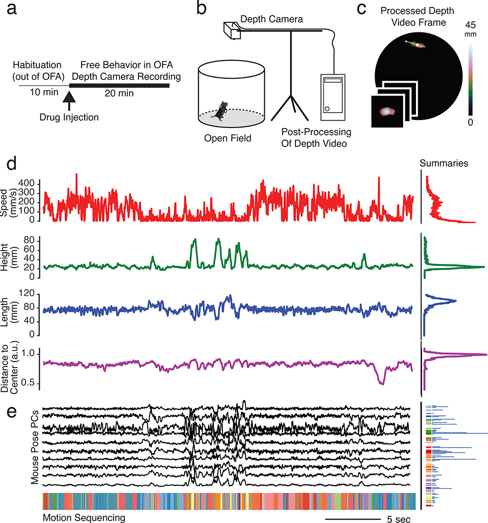
To address whether the modular time-series description of behavior afforded by MoSeq can capture and organize behavioral variation in large-scale data, we acutely exposed mice to a panel of psycho- or neuroactive pharmacological agents at multiple doses known to influence behavior; this drug-based strategy was designed to modulate activity across many neural circuits and neuromodulator systems and to thereby elicit diverse patterns of action in a neutral environment, the circular open field (Figs. 1a–c, n= 673 mice total, Supplementary Table 1).

Fig. 1. Motion Sequencing (MoSeq) captures 3D mouse pose dynamics after drug treatment.

a. Trial structure for mouse open field assay (OFA)-based behavioral imaging.

b. Mouse 3D pose dynamics were recorded using depth cameras placed above the arena, with raw frames stored locally and then processed in a cloud computing environment (see Methods).

c. A pre-processing pipeline identifies the mouse within the depth image, enabling analysis of 3D pose dynamics as well as quantification of scalar behavioral metrics (see Methods).

d. Imaging-based distributions of an example mouse’s speed, height, length and distance to arena center during a 30 second example snippet.

e. The first ten principal components of the pre-processed 3D imaging data (top) were fed to the MoSeq algorithm to assign each frame to a particular behavioral syllable (bottom, see Extended Data Fig. 1). The number of times each syllable is expressed during this 30 second example snippet is represented as a histogram (right); for each mouse a MoSeq-based behavioral summary was generated using 20 minutes of data.

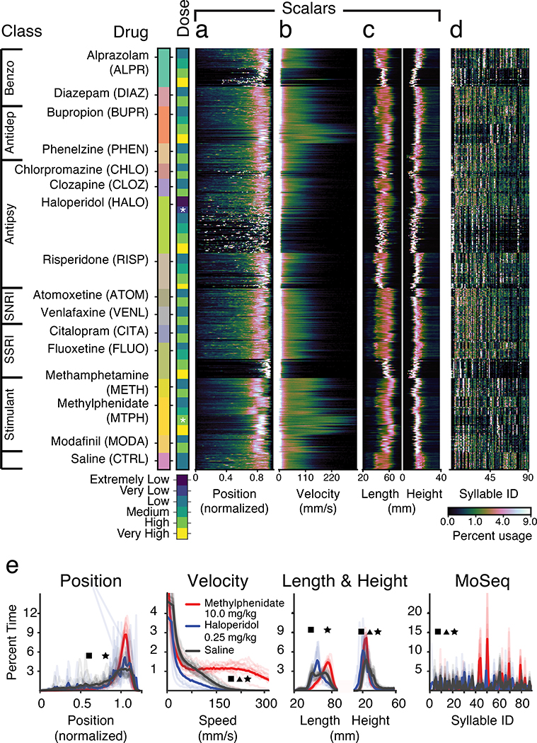
Two distinct behavioral summaries were computed for each imaged mouse. These included a “scalar” summary, composed of parameters typically measured using point tracking over standard 2D video, including distributions of length, speed and position; and a “MoSeq” summary composed of how often each behavioral syllable was used (Figs. 1d–e, 2a–c, see Methods and Extended Data Figs. 1- 2 for details regarding construction of behavioral summaries). Because imaging was performed using 3D cameras, the scalar summary was bolstered by included the centroid height distribution, information not typically available with 2D cameras or beam breaks.

Fig. 2. Generating behavioral diversity though pharmacology.

a. Each mouse (rows) was treated with the indicated drug, and the distribution of mouse positions normalized to the arena center position was computed. Drug class is indicated at left (here and throughout, Benzo = benzodiazepine, Antidep = antidepressant, Antipsy = antipsychotic, SNRI = serotonin non-specific reuptake inhibitor, SSRI = serotonin selective reuptake inhibitor; see Supplementary Table 1 for the number of mice per treatment).

b. Same as a. but for velocity.

c. Same as a. but for length and height.

d. Same as a. but the behavioral summary is composed of how often each MoSeq-identified syllable (arrayed on x-axis) was used.

e. Comparisons of behavioral summaries for methylphenidate, haloperidol and saline at the doses indicated by the stars in the “dose” column in a. (p<0.05, square indicated significant differences between methylphenidate and haloperidol, triangle between haloperidol and saline, and star between methylphenidate and saline; two-sided Mann-Whitney U test is used on mean values for scalars; for MoSeq syllable differences using a two-factor MANOVA; faint lines represent distribution of individual mice).

Visual inspection of the scalar behavioral summaries for each mouse offered intuitive insight into drug-induced behavioral states. For example, high-dose haloperidol caused low average speeds and frequent long-term pausing (apparent as a speckled pattern in mouse position), consistent with its known cataleptic effects²¹ (Figs. 2a, 2b, 2e). In contrast, methylphenidate drove mice to the edge of the arena and substantially increased their velocity, consistent with its known stimulating properties²². MoSeq-based behavioral summaries captured a variety of sub-second stereotyped 3D actions (e.g., darts, rears, pauses, turns) that differentiated most drugs and doses from control (Figs. 2d, 2e, mean duration ± SD = 425 ± 726 ms, see Extended Data Fig. 3 for descriptions of behavioral syllables).

MoSeq enables effective behavioral classification

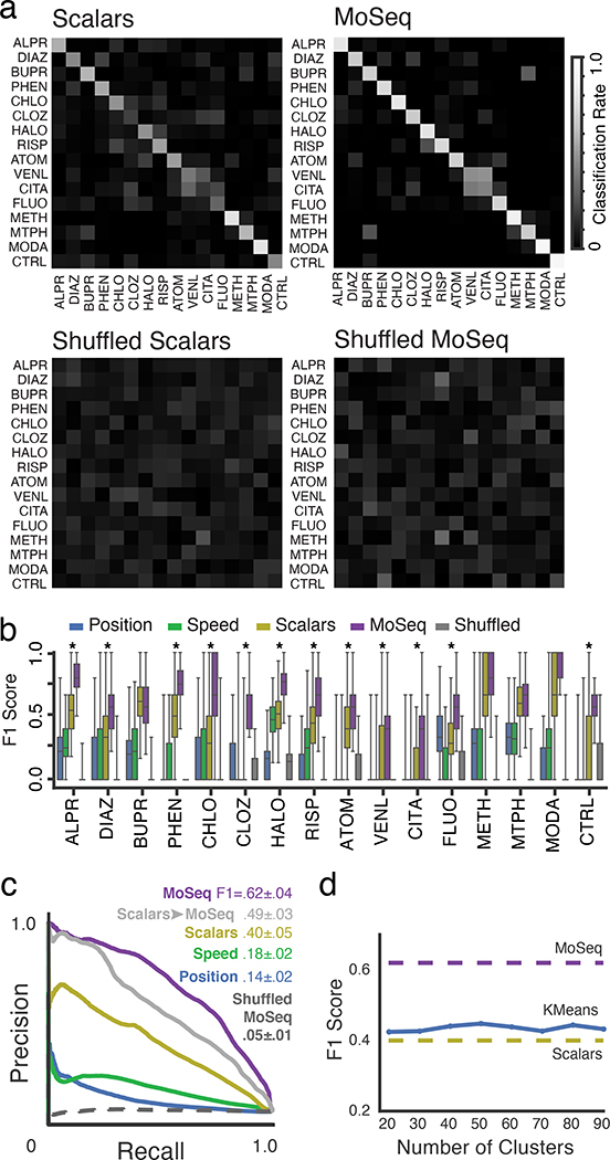
Scalar and MoSeq behavioral summaries for each mouse were submitted to a linear classifier to quantify the ability of each behavioral summary to distinguish each drug. As shown in Fig. 3, MoSeq outperformed traditional summaries at identifying individual drugs based upon behavior (MoSeq F1 = .62 ± .04 vs scalar F1 = .40 ± .05; F1 values represent the harmonic mean between precision and recall, and summarize the ability of a given method to capture true positives while rejecting both false positives and negatives). MoSeq was better at discriminating 14 out of the 16 drugs tested, including the saline controls (Fig. 3b and Supplementary Table 2, see Methods for the use of randomized cross-validation to assess model reliability and statistical significance). Although absolute performance was reduced, MoSeq was also more effective at predicting the specific drug-dose combination each mouse was administered (Extended Data Fig. 4, Supplementary Table 3). Consistent with these classifier-based findings, the effective dimensionality of MoSeq, which measures its intrinsic capacity to describe behavioral variability, was higher than that for scalar metrics (Extended Data Fig. 4c). These experiments demonstrate that each drug elicits a specific pattern of behavior in treated mice, and that — across nearly all drugs tested — MoSeq is more effective at capturing drug-specific behavioral effects than traditional metrics.

Fig. 3. MoSeq discriminates drug-induced patterns of behavior.

a. Normalized classification matrices (across rows and columns, plots represent classifier means after 500 cross-validation folds, see Methods for details and Supplementary Table 1 for number of mice used per treatment) summarizing the performance of a linear classifier at distinguishing different drugs based upon the indicated behavioral summary. Perfect classifier performance (in which each mouse is correctly assigned to its drug label) corresponds to white along the diagonal and black on the off-diagonal (i.e., a classification rate of 1). For the shuffled control (bottom row), drug labels were shuffled on a per-mouse basis to compute a baseline of expected random performance. Heat map indicates classification successes and errors (see Methods for summary definitions). Drug abbreviations here and throughout as indicated in Fig. 2.

b. F1 values, reflecting classification accuracy, for all behavioral summaries, including a label-shuffled random baseline. Box plots represent the distribution across 500 cross-validation folds, with whiskers representing 1.5 times the inter-quartile range. Shuffle controls as in a (p<0.01, paired two-sided t-test, Holm-Bonferroni step-down correction; stars indicate statistically-significant differences between MoSeq and scalars)

c. Mean precision-recall curves and F1 values for all summary types across all drug treatments. Shuffle controls as in a. “Scalars -> MoSeq” indicates performance observed when modeling scalar values rather than 3D imaging data using MoSeq.

d. Mean F1 score of an alternative behavioral summary, constructed by performing KMeans clustering (with cluster number indicated) on the 3D image principal components (see Methods). Note that the MoSeq summaries are composed of 90 syllables, which corresponds to the maximum number of clusters chosen for analysis here. For comparison, mean F1 predictive performance scores are indicated for MoSeq and scalars.

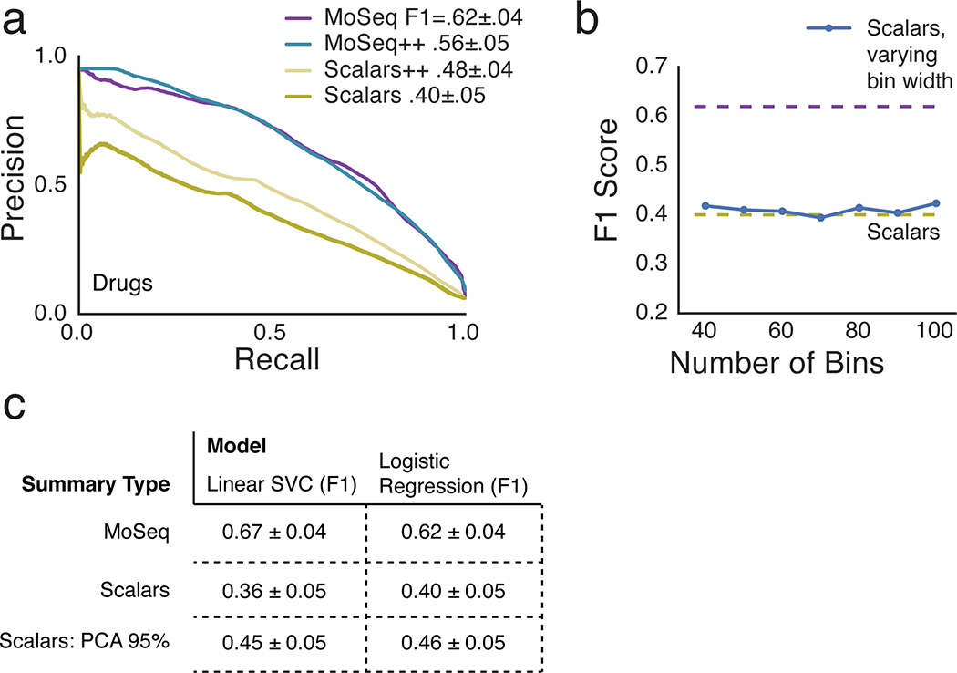
The data that make up each behavioral summary constrain its ability to convey information about behavioral variability, raising the possibility that the specific composition of each summary limits its performance. To address this possibility, we modified both the scalar and MoSeq summaries to include additional measurements that were excluded in our initial analysis (such as acceleration, body angle, area, ellipticity and width in the case of scalar summaries, and syllable transition information for MoSeq). In neither case did performance exceed that of syllable usage-based MoSeq alone (Extended Data Fig. 5a). In addition, MoSeq outperformed scalar metrics regardless of whether the scalar data were subject to dimensionality reduction, whether the scalar data were lumped into more or fewer bins, or whether alternative classifier types were used to assess performance (Extended Data Figs. 5b and 5c).

These observations suggest that the time-series modeling approach used by MoSeq captures more relevant behavioral variance than simply aggregating behavioral data into histograms (as done by the scalar behavioral summary). To assess the importance of time-series modeling per se, we fed the frame-by-frame values of the parameters that make up the scalar behavioral summary to MoSeq, thereby identifying “syllables” based upon scalar measurements instead of the 3D imaging data. This hybrid scalar/MoSeq summary exhibited improved performance relative to the scalar summary, and yet was still worse than classification performed using 3D imaging data (Fig. 3c). We also subjected the 3D pixel data to KMeans clustering, thereby generating a summary in which behavior is characterized by how often mice adopt one of many possible 3D poses; this KMeans summary, in which behavior was clustered without regard to time, also significantly underperformed MoSeq (Figure 3D). These findings demonstrate that time-series modeling can substantially improve the performance of even simple scalar metrics, and that the 3D pixel data describing the mouse’s full pose dynamics contribute information important to behavioral classification that is absent from scalar metrics alone.

MoSeq separates treatment groups while capturing individual variation

Why is the behavioral summary generated by MoSeq effective at discriminating between closely-related patterns of behavior? In principle, there are two (non-mutually exclusive) possible reasons. First, MoSeq might primarily act to separate treatment classes (here, mice treated with a given drug or drug/dose combination); if this were the case, the separation among the mean MoSeq behavioral summaries for each class should be large, and greater than that observed when using scalar behavioral summaries. Alternatively, the mean class separation could be similar among summary types, but MoSeq might generate summaries with relatively low mouse-by-mouse variability, thereby reducing the confusion between drugs when assessed by the classifier.

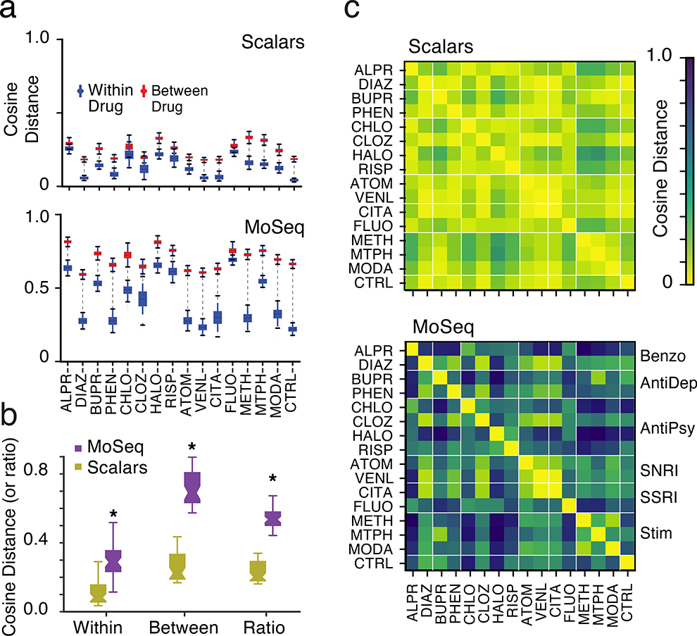
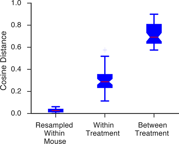
To explore these possibilities, we quantified the cosine distance that separated MoSeq summaries, and compared these distances to those observed using scalar summaries. This analysis revealed that the mean separation between mice treated with different drugs, or drug-dose combinations, was greater when using MoSeq (Figs. 4a and 4b, Extended Data Fig. 6). Surprisingly, the cosine distances that separate individual mice within a given treatment class — i.e., which all received the same drug — were also greater when using MoSeq than when using scalar summaries (Figs. 4a and 4b). Bootstrapping analysis demonstrated that these greater distances were not due to noise, but rather to bona fide behavioral differences between individual mice belonging to the same treatment class (Extended Data Fig. 7). Together these results demonstrate that MoSeq supports behavioral classification by increasing the separation (relative to other metrics) between different treatment groups, while at the same time maintaining information about the behavioral variability of individual mice within each treatment group.

Fig. 4. MoSeq enhances the separation between treatment classes relative to scalars.

a. Average cosine distances of individual mice given the same drug (blue) compared to mice given different drugs (red, ±1 standard deviation indicated; see Supplementary Table 1 for number of mice used per treatment).

b. Mean within- and between-treatment cosine distances, and their ratio, for scalar summaries and MoSeq (p<0.05, stars indicate significant difference between MoSeq and scalars, paired two-sided t-test).

c. Average pairwise cosine distances between mice given indicated drug treatments (distance indicated by color bar; lines separate drug classes indicated to right of lower panel).

MoSeq reveals behavioral relationships in large-scale datasets

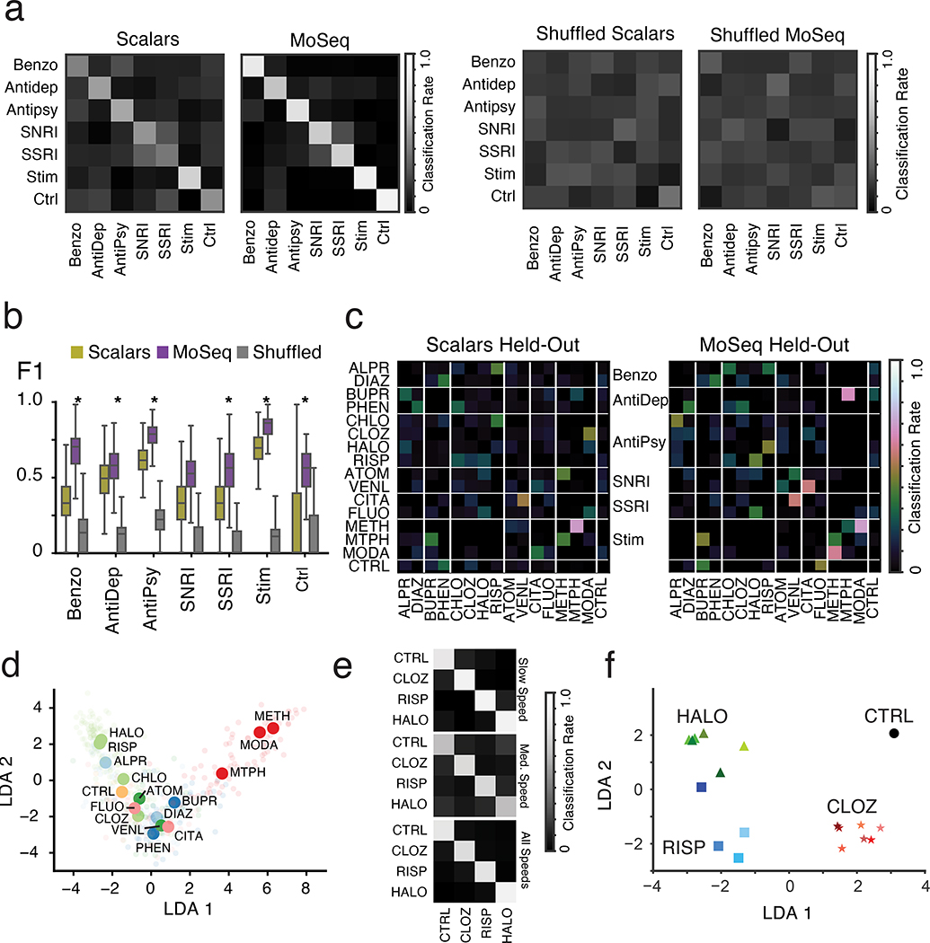
These findings indicate that MoSeq effectively distinguishes patterns of behavior imposed by specific drugs. However, it is not clear whether MoSeq also captures information about drug-related behaviors that are shared across drugs, which could be diminished if MoSeq simply decorrelates representations for each mouse’s behavior; indeed, the greater overlaps between the representations of individual mice observed in the scalar summaries (Fig. 4c) could enable those summaries to better represent behavioral relationships. However, classifier analysis revealed that MoSeq was uniformly more effective than traditional metrics at identifying the pharmacological class to which a given drug belongs (moSeq F1 = .65 ± .04, scalar F1 = .42 ± .06, chance F1 = .12 ± 02, Figs. 5a and 5b).

Fig. 5. MoSeq reveals behavioral relationships between drug classes and can distinguish catalepsy from sedation.

a. Normalized classification matrices (across rows and columns, plots represent means after 500 cross-validation folds, see Methods) summarizing classification performance of linear classifiers trained to predict drug class on a mouse-for-mouse basis (left). Heat map indicates classification successes and errors; perfect classifier performance (in which each mouse is correctly assigned to its class label) corresponds to white along the diagonal and black on the off diagonal (i.e., a classification accuracy of 1). For the shuffled control (right), class labels were shuffled on a per-mouse basis to compute a baseline of expected random performance. See Supplementary Table 1 for number of mice used per treatment.

b. F1 scores for linear classifiers designed to predict pharmacological drug class on a mouse-for-mouse basis. Box plots represent the distribution across 500 cross-validation folds, with whiskers representing 1.5 times the inter-quartile range (p < .01, stars indicate significant differences between MoSeq and scalars, paired two-sided t-test corrected with Holm-Bonferroni step-down procedure, see Methods). Shuffle control performed as in a.

c. Held-out confusion matrices (across rows and columns) indicating the classification of a given drug when that drug was excluded from the drug classifier (and thus these matrices represent confusions made over 16 separate classifiers). This procedure identifies the drugs most confused with the query drug (given that, by design, the held-out classifier must identify a non-query drug as the correct label for each mouse). As correct within-drug classification is impossible in this representation, the diagonal is dark (plots depicts means after 500 cross-validation folds, see Methods for details of “held-out” classification, drug classes are indicated).

d. Linear discriminant analysis (LDA) plot indicating the similarity between the mean behavioral summaries of mice across drug treatments. Opaque circles indicate mean summary embeddings, and semi-transparent circles show the embedding location of each mouse. Colors indicate drugs from the same pharmacological class.

e. Normalized classification matrices for different drugs, where the specific doses chosen for each drug were grouped based upon mouse speed (mean centroid speed of saline control mouse = 74 mm/sec; “medium speed” = 54 mm/sec; “slow speed” = 24 mm/sec; see Methods for description of Gaussian Mixture Model-based method for grouping doses based upon speed). Perfect classification is indicated by white along the diagonal and black off diagonal; the high degree of predictability when stratifying different below normal speeds demonstrates that MoSeq can distinguish these drugs independent of their effects on gross movement.

f. LDA plot indicating the observed mean MoSeq-characterized pattern of syllable usages for the three indicated drugs (green = haloperidol, red = clozapine, blue = risperidone) at doses tiling very low (light) to very high (dark, see Methods). In general, all doses of each drug cluster together in LDA space, and separate from a control saline treatment, although at the highest doses risperidone and haloperidol elicit similar patterns of behavior (see darkest blue square and darkest green triangle).

Given that the notion of pharmacological class is not rigorous — as many drugs used in neurological and psychiatric practice are deployed for indications that cross diagnostic boundaries²³ — we asked whether MoSeq or scalar behavioral representations could identify behavioral relationships independent of constructed categories. Indeed, the pairwise correlation matrices describing behavioral similarities and differences revealed behavioral relationships between drugs across distinct pharmacological classes (Fig. 4c). To explore drug relationships from a classification perspective, we removed a single drug from our dataset, and then built a linear classifier based upon the MoSeq or scalar summaries of the remaining drugs to identify those agents that were most behaviorally similar to the “held-out” drug. By iteratively holding out each drug in the set, we could identify overlaps in the patterns of behavior evoked by all drugs in our dataset, and then compare the overlaps identified by MoSeq and scalars (Fig. 5c).

When applied to MoSeq summaries, this approach identified relationships among drugs that belong to the same class (e.g., modafinil/methamphetamine, haloperidol/risperidone), and as well three prominent inter-class relationships (e.g., methylphenidate (stimulant) /bupropion (anti-depressant), venlafaxine (SSRIs) /citalopram (serotonin non-selective reuptake inhibitor) and chlorpromazine (anti-psychotic) /alprazolam (anxiolytic)). These same drug relationships were observed when embedding the MoSeq behavioral summaries into a two-dimensional space using Linear Discriminant Analysis for visualization purposes (LDA, Fig. 5d), but were weaker or absent when held-out confusion matrices were computed using scalar summaries. Interestingly, data-mining revealed that two of the inter-class pairs share clinical indications, while the third pair (alprazolam/chlorpromazine) shares sedation as a side effect²³ (Supplementary Table 4, see Methods). Thus, MoSeq identifies relationships amongst drugs that both include and transcend traditionally-defined pharmacological classes; these behavioral relationships may in part reflect the observed effects of drugs in the clinic.

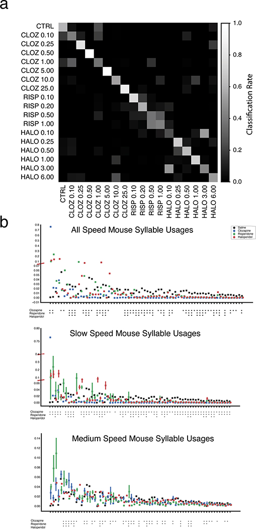
To pressure-test the notion that MoSeq can simultaneously capture useful information about behavioral similarities and differences, we generated dose response curves for three anti-psychotic drugs — haloperidol, clozapine and risperidone — that all elicit a reduction in movement, albeit through different mechanisms; haloperidol and risperidone both antagonize the dopamine D2 receptor (D2R) and therefore trigger catalepsy, while clozapine and risperidone inhibit the 5-HT_2A receptor (5-HT_2AR), which is thought to lead to sedation^24,25. Clozapine is also a high-affinity histamine H1 receptor antagonist, which contributes to its sedative effects^24,25. Consistent with each of these agents antagonizing different receptors with distinct affinities^24,25, classifier analysis demonstrated that MoSeq effectively distinguished nearly all drug-dose combinations (Extended Data Fig. 8a). Each drug altered a specific complement of behavioral syllables, many of which were unrelated to locomotion — e.g, grooming, rearing (Extended Data Fig. 8b); consistent with this observation, MoSeq could effectively classify the three drugs independent of their differential effects on velocity (Fig. 5e). Embedding the dose-response data using LDA revealed that at high doses risperidone and haloperidol converged upon a similar pattern of behavior distinct from that evoked by clozapine (Fig. 5f, compare darkest blue square, green triangle and red star). These results demonstrate that MoSeq can differentiate between catalepsy (i.e., haloperidol-typical behaviors) and sedation (i.e., clozapine-typical behaviors), which both reduce movement and are often confused in traditional behavioral assays²⁶; the fact that at high doses risperidone acts predominantly as a cataleptic rather than a sedative suggests that its primary behavioral effects at high doses are caused by antagonism of the D2R rather than the 5-HT_2AR (despite the higher affinity of risperidone for the 5-HT_2AR relative to the D2R); importantly, this inference (drawn based upon MoSeq analysis alone) is consistent with the previous finding that locomotion is persistently reduced by risperidone in 5-HT_2AR knockout mice²⁶.

MoSeq identifies subsets of behavioral syllables that encapsulate phenotypes

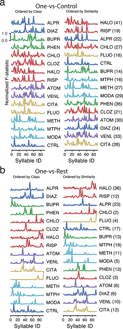
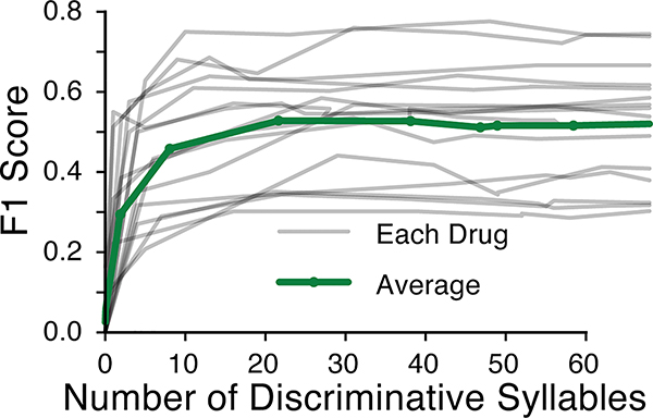
The ability of MoSeq to effectively distinguish drug effects while maintaining information about related patterns of behavior raises the question of how drug treatments alter the pattern of expression of behavioral syllables. Each drug appeared to significantly alter a large subset of syllables when considered relative to control (Fig. 6a). However, LASSO regression revealed that most of the information required to tell individual drugs apart from each other resides in a small subset of syllables (typically 5, nearly always fewer than 15, Extended Data Fig. 9). These small groups of drug-characteristic syllables reflected the similarities and differences between drugs as identified via the “held-out” classifier, including within drug-class relationships (e.g., modafinil/methampehtamine) as well as across-class relationships (e.g., citalopram/venlafaxine) (Fig. 6b, see Supplementary Figs. 1, 2 for a description of similarities and differences among drug-regulated and discrimination-relevant syllables).

Fig. 6. Subsets of syllables fingerprint each drug.

a. A normalized F statistic identifies the quantitative relevance of each indicated syllable for discriminating a given drug treatment from a control saline treatment; ordering on left is based upon pharmacological class, ordering on right is based upon similarities in the F statistic-identified syllables. The number of significant syllables is indicated next to the drug treatment name on the right (Holm-Bonferroni corrected p<0.01 from the two-sided F-test). The control treatment F statistic is computed by comparing against all other treatments.

b. Same as a. but computing the F statistic between a given drug treatment and all other treatments; the all-vs-all comparison reveals many fewer statistically-significant syllables than when comparing to control alone. Note that those syllables that distinguish a given drug from control can be distinct from those that maximially distinguish a particular drug from all other tested drugs.

In accord with its known role as a stimulant, all of the five most discriminant methamphetamine-related syllables encoded different forms of forward movement; three of these syllables overlap with the five most discriminant syllables for modafinil, with the two modafinil-specific syllables encoding exploratory behaviors, including a partial rear and a pause-and-head-flick motif (Supplementary Fig. 3). These observations demonstrate that modafinil shares at least some stimulant-related activity with methamphetamine, consistent with modafinil and methamphetamine acting through an overlapping set of molecular targets^27,28; however, modafinil also recruited additional investigatory behaviors, consistent with modafinil engaging receptors distinct from those recruited by methamphetamine. Similarly, citalopram-related syllables encode forward movement and grooming behaviors; a subset of these syllables are shared with venlafaxine, which also recruited pausing and rearing behaviors not differentially up-regulated by citalopram (Supplementary Fig. 4).

Behavioral syllables enable objective assessment of interactions between genes and candidate therapeutics

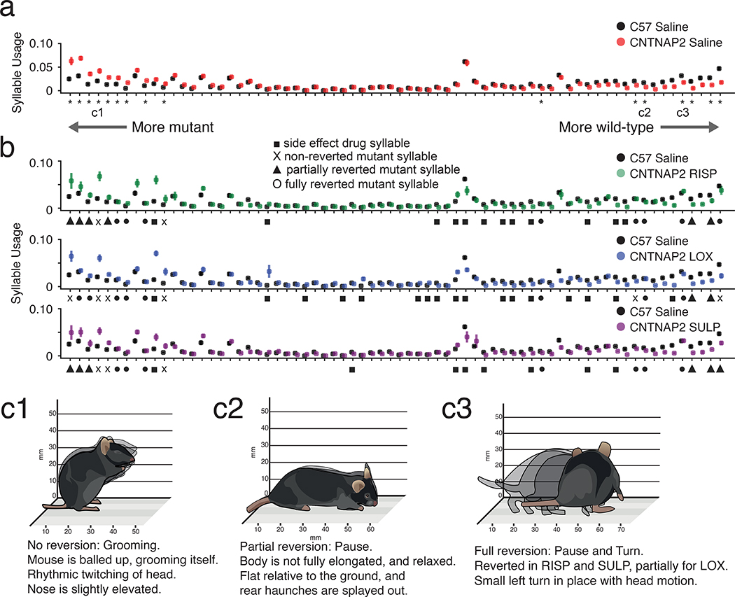
Given its ability to identify specific drug-related behavioral effects, we asked whether MoSeq could characterize the ability of a drug to revert behavioral phenotypes in a disease model. To explore this possibility, we used MoSeq to phenotype mice mutant for the CNTNAP2 gene, which is associated with human autism^20,29,30. Consistent with prior results, velocity measurements revealed that the CNTNAP2 mice are hyperactive^20,31 (Supplementary Fig. 5). MoSeq identified 16 behavioral syllables whose expression is statistically altered with respect to wild-type mice (Fig. 7a). Visual inspection revealed that many of these syllables would be predicted to be associated with a “hyperactive” phenotype (e.g., downregulated pauses, and upregulated micromovements and running); however, many high-velocity syllables were not affected by the CNTNAP2 mutation (data not shown), demonstrating that CNTNAP2 hyperactivity does not reflect generalized arousal, but instead is composed of a specific array of syllabic changes (Fig. 7a).

Fig. 7. MoSeq-based phenotypic fingerprinting reveals on- and off-target drug effects in a mouse model of autism spectrum disorder.

a. Usage plots for wild-type (black) and Cntnap2 −/− (red) mice injected with saline control (bootstrapped 95% confidence intervals indicated). Syllables sorted by the degree to which they are overused in the mutant (see Methods), with differentially used syllables marked by asterisks (for all statistical tests in this figure, Kruskal-Wallis and post-hoc Dunn’s two-sided test with permutation, with Benjamini/Hochberg FDR with alpha = 0.05). Example syllables illustrated in c are indicated as c1, c2 and c3. See Methods for number of mice per treatment group.

b. Usage plots for wild-type (black) and Cntnap2 −/− mice injected with risperidone (RISP; green), loxapine (LOX; blue) and sulpiride (SULP; purple). Symbols indicate differentially used syllables (circle: fully reverted mutant syllable, triangle: partially reverted mutant syllable, cross: not reverted mutant syllable; square: drug-induced side-effect syllable, see Methods for definitions of reversions and side effects).

c. Schematic illustrations of syllables that were either not reverted (c1), partially reverted (c2) or fully reverted (c3) by drug treatments. Note that syllable c3 was fully reverted with RISP and SULP, but only partially reverted with LOX.

Previous experiments have shown that the CNTNAP2 hyperactivity phenotype can be reverted by treatment with risperidone, which is used clinically to treat hyperactivity and aggression in autistic patients²⁰. Of the 16 behavioral syllables that define the CNTNAP2 mutant phenotype, seven were statistically normalized by risperidone treatment, seven were partially reverted and two remained uncorrected (Figs. 7a–c). Despite not fully reverting the observed mutant phenotype, risperidone also altered a large number of additional behavioral syllables, several of which represent high velocity behaviors like running. These results quantitatively demonstrate that risperidone has a specific (albeit partial) effect on the phenotype induced by mutation of the CNTNAP2 gene, and a much broader set of side effects on normal behavioral syllables.

We also wished to test the utility of MoSeq for characterizing the on- and off-target effects of novel or previously-untested therapeutics in the CNTNAP2 model; to identify candidates, we took advantage of a repurposing dataset in which possible ASD therapies were nominated based upon the intersection of genome-wide association data and drug-induced changes in gene expression³². From this list we identified two drugs, loxapine and sulpiride, that have not been previously tested in CNTNAP2 mutant mice and whose mechanisms of action overlap with — but are distinct from — risperidone (loxapine also antagonizes both the D2R and 5-HTR_2A, but with a lower relative inhibition ratio than risperidone³³, while sulpiride is a pure D2R antagonist).

Like risperidone, both sulpiride and loxapine reverted the gross hyperactivity of the CNTNAP2 mutant mice, as assessed by velocity measurements (Supplementary Fig. 5). However, MoSeq revealed that loxapine was less efficacious than risperidone at correcting CNTNAP2-specific syllables, and further recruited more side-effect syllables. In contrast, sulpiride exhibited nearly identical on-target effects with risperidone, but altered fewer off-target syllables (Figs. 7a–c); importantly, with one exception the off-target syllables induced by sulpiride — which specifically antagonizes the D2R — overlapped with the broader set induced by risperidone. These data suggest that D2R antagonism is sufficient to revert the CNTNAP2 phenotype, and further that the risperidone-specific off-target effects (relative to sulpiride) are likely due to antagonism of other receptors, such as the 5-HT_2AR (Supplementary Figs. 5 and 6). These experiments reveal that MoSeq can identify a syllabic fingerprint that characterizes complex behavioral changes in a disease model; this fingerprint can be usefully used both to quantitatively assess the intended and inadvertent effects of candidate therapeutic agents, and to deconvolve relationships between drugs, receptors and behavior.

Discussion

Before these experiments it was not apparent whether MoSeq is more like a Northern blot — a bespoke approach for understanding the relative expression levels of a small number of target RNAs from a limited set of samples — or RNASeq, which creates a broad and general representation of the transcriptome that can be effectively used to infer relationships amongst many different cell types and experimental interventions. This work reveals that MoSeq can parse experimentally-induced behavioral variability within large-scale and diverse datasets. Despite the fact that MoSeq is highly discriminative — and therefore can identify the specific behavioral effects of closely-related drugs and doses — it retains information about behavioral relationships, allowing drug categorization independent of presumed mechanism of action. These features also enable MoSeq to unveil the intersecting effects of gene and drug manipulations, even when the mechanistic consequences of those interventions are incompletely understood.

Drugs act at specific complements of receptors that selectively modulate the activity of neural circuits, which in turn cause changes in behavior. However, efforts to link drug effects to molecular mechanisms and behaviorally-relevant circuits have been significantly complicated by the low dimensionality, poor signal-to-noise, and lack of specificity of traditional behavioral metrics. The discriminative capacity of MoSeq suggests that it may ultimately enable receptor modulation to be causally mapped onto patterns of neural circuit activity and behavior, thereby allowing inferences to be drawn about the role of drug receptors in composing and shaping behavioral space. Our proof-of-concept experiments provisionally linking the differential expression of particular syllables to the modulation of specific receptors (made possible by phenotyping different drugs with distinct but overlapping receptor specificities) suggest that this sort of mapping could also enable accurate predictions of drug mechanism of action from behavior alone.

We speculate that MoSeq outperforms traditional behavioral representations for four reasons. First, MoSeq organizes information about 3D pose dynamics based upon the inherent structure of the behavioral data, and in a manner that respects the observation that mouse behavior is both continuous and discrete. Second, MoSeq does not prespecify the number and identity of behavioral syllables, but instead learns these features on an experiment-by-experiment basis. Thus, the richness of the behavioral representation scales with the amount of observed behavioral variability, enabling MoSeq to summarize behavior in a manner that is simultaneously compact and expressive^9,34. Third, MoSeq defines individual syllables in part based upon the order in which they occur, and thus leverages the sequential nature of naturalistic behavior^3,35–37. And finally, recent work suggests that the dorsolateral striatum encodes syllable identity and is required to assemble syllables into coherent sequences¹¹. Thus MoSeq may be particularly effective because it describes behavior, at least in part, in modular terms similar to those used by the brain to create it.

We explicitly chose to measure behavior in experiments in which mice explore featureless environments after acute drug exposure, reasoning that this represented a ground state in which behavioral differences should be difficult to quantify, thereby putting MoSeq to a rigorous test. It is clear that different patterns of behavior would be observed if mice were given drugs chronically rather than acutely, or placed in richer contexts that demand goal-oriented behaviors. For example, one might expect chronic methamphetamine (which is highly addictive) and chronic modafinil (which is not) to be more distinguishable than was observed here with acute treatment alone²³; similarly, drugs that influence frontal circuits (like anti-psychotics) might elicit greater behavioral differences in the context of social or stress assays. Furthermore, the relatively brief experiments carried out here almost certainly fail to capture the ability of many drugs (and associated neural circuits) to reshape behavior over long timescales. Future work will be required to assess the utility of MoSeq in long-term behavioral assays or in assays designed to elicit specific psychological reactions, like the forced swim test or three chamber social assay.

Many of the chemical templates for currently used psychotherapeutics were discovered in the 1950s and 60s based upon their behavioral effects³⁸. This led to the widespread use of behavioral phenotypes (ranging from open field entries to spider web geometry) to screen for candidate therapeutics^39,40; however, limited by low resolution and high variability, these behavior-based approaches have generally failed to yield novel pharmacology. More recent drug development efforts have focused on identifying risk genes and using medicinal chemistry to actuate or inhibit those specific targets. This alternative strategy has also not been entirely successful, perhaps in part because most clinically-approved neuro- and psychotherapeutics exhibit mixed selectivity for multiple targets^23,25,38. The observation that MoSeq summarizes complex behavioral phenotypes induced by drug and genetic manipulations — which almost certainly exert their effects through many receptors and neural circuit mechanisms in parallel — as discrete changes in subsets of behavioral syllables suggests that syllables themselves could serve as druggable targets. The ability of MoSeq to reveal on- and off-target effects of risperdone, sulpiride and loxapine in CNTNAP2 mutant mice is consistent with this possibility. Given its low cost, scalability, and interpretability, MoSeq may be useful as a discovery platform for characterizing the specific disease-relevant effects of candidate therapeutics.

Methods

Ethical Compliance

All experimental procedures were approved by the Harvard Medical School Institutional Animal Care and Use Committee (protocol number 04930) and were performed in compliance with the ethical regulations of Harvard University as well as the Guide for Animal Care and Use of Laboratory Animals.

Data Acquisition

Drugs were tested on n=673 6–8 week old C57/BL6 males (Jackson Laboratories). Mice were housed in standard animal facility conditions, at a temperature of 71 ± 3 degrees, and at a relative humidity of 50 ± 15 percent. Mice were introduced into the colony at five weeks of age, and group-housed for one week in a reverse 12 hours light/12 hours dark cycle. On the day of testing, mice were brought into the laboratory in a light-tight container, where they were habituated to the experiment room under red light for 10 minutes in disposable cages (Innovive) containing fresh bedding, with food and water available ad libitum. After the habituation period and subsequent drug injection, mice were placed in the middle of a circular 18” diameter open field assay (OFA) enclosure with 15”-high opaque walls (US Plastics), immediately after which video recording was begun. All experiments were performed under red light. Mice were allowed to freely explore the enclosure for the 20 minute experimental period. At the end of the experiment the enclosure was cleaned with 70% ethanol before reuse.

Drug treatments

Each mouse was treated with a single drug/dose combination, and used only once. Drug names, their concentration, the method used for dilution, the number of mice treated with each drug/dose combination, and supporting citations for the choice of dose are described in Supplementary Table 1. Drug doses were selected based upon the published literature to maximize the likelihood of observing a behavioral effect within the dose-response window. All drugs were delivered via intraperitoneal (IP) injection. All drug dilutions were prepared fresh on the day of experimentation, dissolved in accordance with previously published work, and delivered IP in a final volume of 200 μl. Drugs were generally diluted in lactated ringers solution (LRS), except for fluoxetine (at doses higher than 10 mg/kg), haloperidol (at doses higher than .25 mg/kg), and methylphenidate, which were diluted in ddH₂O. In instances where a drug was not soluble in LRS or ddH₂O, the drug was first diluted in Dimethyl Sulfoxide (DMSO), then further diluted in LRS. Drug-dose pairs were tested in pseudorandomized order, with control mice interspersed with drug treatments throughout the data acquisition phase of the experiment. The data acquisition phase of the experiment lasted for a period of 12 weeks (excluding the CNTNAP2 experiments). Data collection and analysis were not performed blind to the conditions of the experiments. No statistical methods were used to pre-determine sample sizes, but our sample sizes are similar to those reported in previous publications¹.

CNTNAP2 mutant mouse experiments

Male wild-type or mutant littermates from breeding pairs of heterozygous CNTNAP2 mutants (JAX stock No. 017482) were subjected to acute drug or saline injections as described above. Data from mice included in the analysis (for wild-type mice, n=39 with saline, n=20 with .1 mg/kg risperidone, n= 4 with .5 mg/kg loxapine, n=8 with 20 mg/kg sulpiride; for CNTNAP mice, n=9 with saline, n=4 with risperidone, n=6 with loxapine, n = 5 with sulpiride) were modeled separately from the remainder of the drug data (see below).

Behavioral Recording

Data acquisition was performed identically as in Wiltschko et al⁹, using three parallel set-ups to maximize throughput. Mice were tracked in 3D using a Kinect for Windows v1 (Microsoft). This camera projects structured infrared light onto the imaging field, and the three-dimensional position of objects in the imaging field are computed based upon parallax. A boom tripod (Manfrotto) was used to suspend the camera above the recording arena, affording a stable top-down view of the mouse. The Kinect v1 has a minimum working distance (in Near Mode) of 0.5 meters; by quantitating the number of missing depth pixels within an imaged field, we have found that the optimal sensor position data is between 0.6 and 0.75 meters depending on ambient light conditions and assay material.

Data from the Kinect was sent to an acquisition computer (hand-assembled, 16GB RAM, Intel i7 CPU, 512GB SSD) via USB. A custom Matlab script was used to interface the Kinect via the official Microsoft .NET API that retrieves depth frames at a rate of 30 frames per second and saves the frames in raw binary format (16-bit unsigned integers) to disk. Relevant experimental metadata (mouse ID, drug ID and dose) was captured and saved in the same folder name into which the raw binary depth data recorded to disk. Because USB 3.0 has sufficient bandwidth to allow streaming of the data to an external hard-drive in real-time, hot-swappable external hard drives were used for all data storage. After the completion of the experiment, a region-of-interest (ROI) was specified to delineate the area where the mouse could feasibly explore. This polygon was saved alongside the depth data, and used to simplify the data extraction process by eliminating pixels outside the arena.

Data preprocessing and extraction

Raw frames recorded to external hard drives were immediately copied to the network-attached storage (NAS) associated with the Harvard Medical School Orchestra cluster. Custom mouse tracking software was then run to extract the mouse’s position, orientation and body morphometry from the raw depth data. All extraction software was implemented in the Python programming language, using the MPI4Py, H5Py, joblib, pandas, OpenCV, Scikit-Learn, Scikit-Image, MoviePy, NumPy and SciPy libraries.

To extract and align the 3D image of the mouse from the video data, raw frames depth frames were first read in as rectilinear blocks of unsigned 16-bit integers, and then these bits were shifted right by three places, yielding distance measurements in millimeters. A background image, used for background subtraction, was then calculated by taking the median value of the first 1000 frames of the recording. Noise in the depth image is highly-correlated in both space and time, due to the structured-illumination technique used to acquire depth information. Missing data was imputed by replacing missing depth pixel values with the spatially nearest valid pixel, in both space and time. The raw depth images were resampled so that every pixel covered 2 square millimeters, using the published properties of the camera’s field-of-view. The resampled images were re-centered by subtracting them from the background image, yielding values indicating how high a given pixel is above the baseline background image. All negative values (portions of the image below the background, usually occurring because of spurious noise), were set to zero. All values above a maximum height (200 mm) were set to zero. Objects above the background that were smaller than a mouse were removed with morphological image operations, using the Scikit-Image “remove_small_objects” and “binary_opening” functions. After these cleaning operations, the largest contiguous group of non-zero values in each frame is the mouse’s body, which was identified with the OpenCV “findContours” function. From this contour polygon, the area, center-of-mass, orientation, and, using the “fitEllipse” function from OpenCV, the best-fit ellipse for each mouse was calculated. A square view measuring 120 mm x 120 mm centered on the mouse was then extracted in every frame, using the mouse contour’s center-of-mass and orientation; the major axis of the ellipse defining the mouse was oriented along the horizontal axis of the square view.

Although in an ideal case this procedure would yield a square field of view in which a mouse was aligned horizontally along the virtual axis of its spine, in reality the best-fit ellipse is not necessarily oriented in the direction of the mouse’s head. To correctly identify the head of the mouse, a random forest classifier was generated using Scikit-Learn, and trained on a corpus of several thousand hand-oriented extracted mouse images. After acquiring a properly-oriented extracted mouse image, and associated contour and positional data, the resultant aligned mouse movie was written to an HDF5 file. To accelerate the extraction process, the extraction over overlapping time-chunks of the experiment was parallelized using MPI. A single mouse’s recording was extracted into a single HDF5 file, and for convenience, all mice were concatenated together into one central HDF5 file, containing the entirety of the recorded data used in this study.

Data Modeling

Once extraction of all experiments completed, the extracted data contained in a single HDF5 file was moved to a customized Starcluster on-demand high-perfomance compute cluster, hosted on Amazon Web Services Elastic Compute Cluster (EC2). Many of the processing steps either benefit from many CPU cores, or require a very high memory budget, so much of the analysis was performed on an x1.32xlarge EC2 machine, with 128 virtual CPU cores, and 2 terabytes of onboard RAM. All cluster configuration and required code was saved on attached Elastic Block Store drives, and all imported data, and any further results of analyses, were saved on an attached Elastic File System (EFS) drive, which was chosen because it did not require manual reformatting when additional storage was required. Local scratch drives were used for intermediate results that did not need persistence.

The extracted mouse images form a time-series that is 3600 (60 pixels * 60 pixels) dimensional, sampled at 30 frames per second. These data were first dimensionally reduced this data using principal components analysis (PCA). All extracted mouse images were loaded into memory, and the RandomizedPCA model from Scikit-Learn was used to learn a 10-dimensional linear embedding of the image time-series. The principal component (PC) time-series was then whitened across all mice to remove covariance between PC dimensions. The PCs were saved onto EFS to avoid recomputing this step.

An Autoregressive Hierarchical Dirichlet Process Hidden Markov Model (AR-HMM), identical to the model specified in Wiltschko et al⁹, was fit to the whitened PCs. All of the data were fit in a single model, except for the CNTNAP2 data, which was modeled separately. Hyperparameters were validated via held-out likelihood assessment and qualitative inspection. Autoregressive observation distributions were initialized using Empirical Bayes⁴². Kappa, the self-transition bias that controls the average duration of states, was set to produce states with duration distributions whose mode matches an independently-specified changepoint detection model (Extended Data Fig. 3). The number of lags in the autoregressive distribution was selected with an automatic relevance detection prior and yielded the highest held-out likelihood (100 ms or 3 frames, see Wiltschko et al.⁹). As was observed in Wiltschko et al⁹, model output was insensitive to the hyperparameters of the hierarchical dirichlet process prior. State sequences were initialized randomly. After initialization, the AR-HMM fit was burned-in with 1000 iterations of Gibbs sampling, and then a maximum likelihood estimate was found with the Viterbi Expectation-Maximization algorithm. This model fitting procedure yielded 92 syllables capturing 95% of total frames in the main dataset (truncated to 90 syllables for convenience), and 67 syllables capturing 95% of total frames for the CNTNAP2 experiment.

Data Quality Control

Data quality was assessed at several stages of the processing pipeline. First, each video recording was directly inspected to determine whether mouse tracking was successful. If there were persistent periods of the mouse’s orientation being labeled as incorrectly flipped, these frames were added as new training data to the random forest flip classifier, described above, and the extraction procedure was run again. A heatmap of the mouse’s body location over the course of the entire experiment was next examined to identify any sharp boundaries or disproportionately bright areas that might indicate tracking of non-mouse objects. If a non-mouse object was tracked (typically the edge of the arena), the ROI of the experiment was redefined, and the experiment was re-extracted. If, after applying all data quality correction methods listed above, the mouse’s body was not tracked and extracted properly, or more than 5% of total frames were dropped or unavailable, the recording was not used in the dataset or any further analyses.

Generating behavioral summaries

Preprocessed behavioral recordings of mice in the open field were further summarized into fixed-length descriptions of behavior. A variety of summaries were constructed, based upon the following parameters:

Position

The center of a hand-drawn circle demarcating the edge of the OFA was considered the center of the arena. The 2D position of a mouse in the arena was subtracted from the circle center position. A histogram of these values was constructed with 90 bins equally spaced between 0 and 120 pixels.

Speed

Mouse speed was calculated as the absolute magnitude of the first time derivative of the mouse’s 2D position in the arena. A histogram of these values was constructed with 90 bins equally spaced between 0 and 20 px/frame.

Length

An ellipse was fit using the Python bindings of OpenCV to the animal’s top-down body contour in each recorded video frame. The length of the mouse for each frame was determined to be the length of the major axis of this ellipse. A histogram of these values was constructed with 45 bins equally spaced between 20 and 100 pixels.

Height

The animal’s height was determined to be the maximum height of the extracted mouse image in each frame. A histogram of these values was constructed with 45 bins equally spaced between 0 and 60 millimeters.

Length and Height

The histograms of length and height were concatenated into a behavioral summary with 90 dimensions.

Acceleration

Mouse acceleration was calculated as the absolute magnitude of the second time derivative of 2D position in the arena. A histogram of these values was constructed with 90 bins equally spaced between 0 and 5 px/framê2.

Angle

A histogram of mouse orientation was constructed, in degrees, with 90 equally spaced bins between 0 and 360°.

Area

A histogram of the area of the best-fit ellipse to the top-down contour of the mouse was constructed, with 90 equally spaced bins between 0 and 12000 px^2.

Ellipticity

A histogram of the ratio of a given mouse’s length to its width was constructed, derived from the best-fit ellipse of the animal’s top-down contour, with 90 equally spaced bins between 1 and 3.

Width

A histogram of mouse width was constructed, derived from the best-fit ellipse of the mouse’s top-down contour, with 90 equally spaced bins between 20 and 50 pixels.

Scalars

The length, height, speed and position summaries were concatenated together.

Scalars++

We concatenated all of the parameters measured in the scalar summary together with the summaries for acceleration, angle, area, ellipticity and width.

MoSeq

MoSeq summaries were composed of a histogram describing the frequency of use of each of the 90 most-used syllables.

KMeans

We fit a KMeans model (using sklearn.cluster.KMeans method with kmeans++ initialization) on the principal components of aligned mouse images (the input to the MoSeq method) with varying numbers of clusters. The fingerprint was composed of the number of frames assigned to each cluster.

MoSeq on Scalars

We fit an AR-HMM model on scalar data (as opposed to the principal components of aligned mouse images), using a 4-dimensional time-series composed of the animal’s distance-to-center, speed, height and length. To match the dimensionality of MoSeq, 90 states were used. The best-fit state sequence of the time-series data was summarized as a histogram of state frequencies, identically to the MoSeq summary described above.

Summaries are displayed (but not analyzed) in the paper as the square-root of their values, to increase visual dynamic range.

MoSeq-based behavioral distance measurements

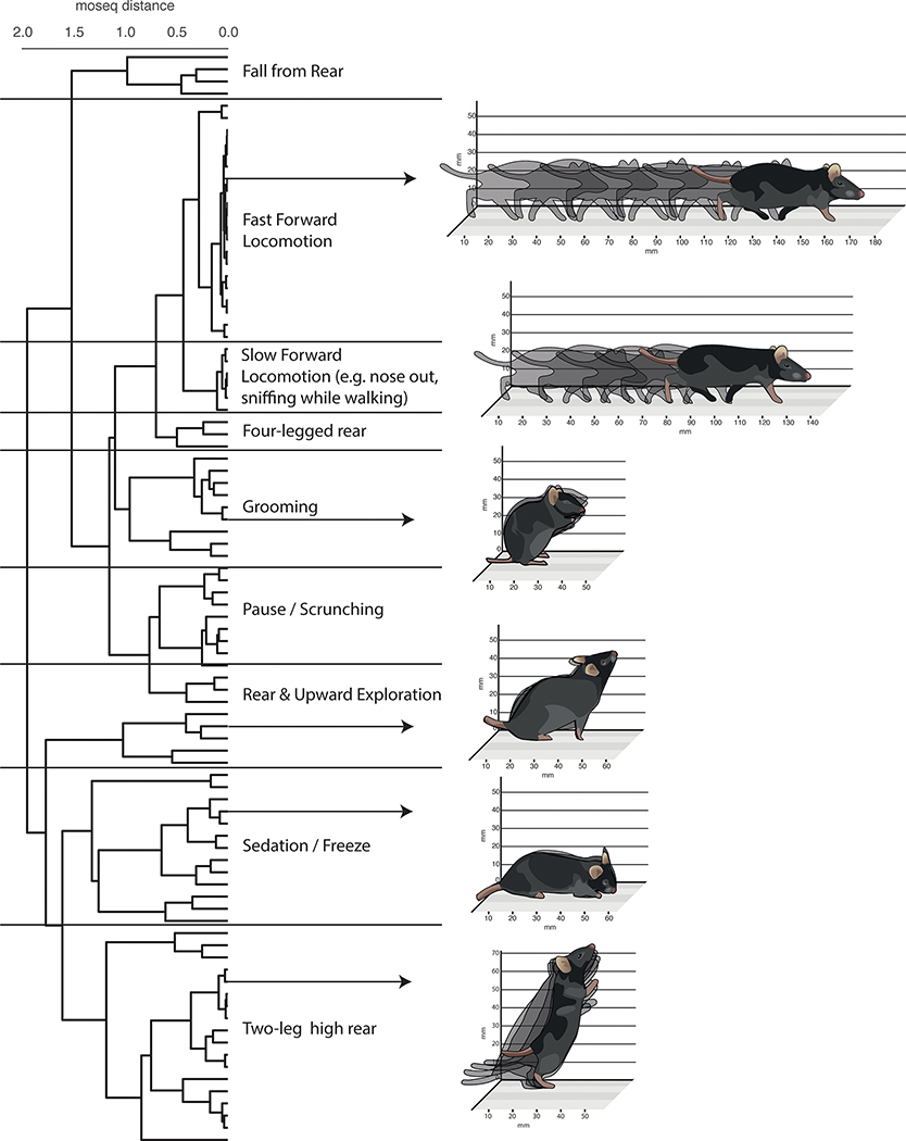
To measure similarity between syllables, we performed MoSeq-based behavioral distance measurements as described in Markowitz et al¹¹. Briefly, we assessed the similarity between pose trajectories of different syllables. We simulated pose trajectories for each syllable over 10 time steps (corresponding to 300ms) using the autoregressive coefficients described by the AR-HMM model fit. Then, we computed the pairwise correlation distance (1 - Pearson’s r) between the top 90 most used syllables to generate a distance matrix, where low distances (near 0) represent similar syllables and high distances (near 2) represent dissimilar syllables.

The cladogram was generated from the distance matrix using the Voor Hees hierarchical clustering algorithm (scipy.cluster.hierarchy.linkage).

Linear classification of behavioral summaries

Classification based upon behavioral summaries was performed using logistic regression as implemented in the Scikit-Learn Python package. The underlying implementation took advantage of the liblinear C/C++ library, using a “one-vs-rest” formulation of multi-class classification. An L2 weight penalty with an inverse regularization strength was also used. We scanned the values 0.01, 0.1, 1.0, 10.0 and 100.0 for each feature type, and presented results for the optimal choice per-feature. To guard against overfitting, 500-fold cross validation was performed, using randomly shuffled folds with 10% of the data held-out per fold, keeping the relative proportion of each label the same in both train and held-out sets. To predict drug identity alone, data from all doses of a given drug were merged, and individual mice were held out. To predict drug class, data from all doses of all drugs belonging to a class were merged. For classification of drug pharmacological class, we also used an additional stratification strategy, where all mice given a particular drug were placed in either the training or held-out set. We observed no appreciable difference in absolute or relative performance (data not shown). The mean and standard error of performance metrics on these randomly-generated held-out folds are reported.

To evaluate performance, confusion matrices, precision-recall (PR) curves, and the F1 score were computed.

Each confusion matrix was a square matrix, with each side length equal to the number of possible target labels, and each square indexed by i,j is the proportion of time a data point with true label i was classified as having label j. When i==j, the classifier correctly predicted the label. Confusion matrices were produced with the confusion_matrix function in Scikit-Learn. Matrices were normalized such that every row and column summed to one, to indicate a probability of classification or misclassification. “Held-out” confusion matrices were calculated by repeating the linear model training and evaluation process N times, where N is the number of treatment groups. For each iteration, one target class was removed from the training set, but added into the held-out set for each fold. This forced the classifier to never correctly classify the removed treatment class, and allowed analysis of the treatments the classifier deemed most similar to the target treatment class. This process was repeated for all treatments to generate the complete “held-out” confusion matrix was plotted.

Precision and recall are quantities computed from the number of true positives, tp, the number of false positives fp, and the number of true negatives tn. Precision and recall are defined as

$$precision=\frac{tp}{tp+fp},recall=\frac{tp}{tp+fn}$$

The PR curve is a plot of the precision and recall of the model, as a decision threshold is varied. The curve is calculated for binary prediction problems by varying the decision threshold for binary predictions (e.g., classifying a mouse as having received a specific drug, versus not having received any other drug), and measuring the false-positive and true-positive rates at that decision threshold for all data in the validation set.

The F1 score is the harmonic mean of precision and recall, and is a measure of binary classification performance:

$$F1=2\ast \frac{precision\ast recall}{precision+recall}$$

The per-label class F1 values were calculated using the f1_score function in scikit-learn. Class-weighted averaging was used across the F1 score of all classes to report a single mean F1 score for a behavioral summary, and standard errors were also calculated.

Behavioral summary distance comparisons

Cosine distance matrix. Distances between two summaries u and v were directly assessed using the cosine distance, computed (using the SciPy Python package) as

$$c(u,v)=1-\frac{u\cdot v}{\left|\right|u\left|{|}_2\right|\left|v\right|{|}_2}$$

The cosine distance was used because it is bounded between 0 and 2, allowing comparisons between behavioral summaries with different units. Within- and between-treatment cosine distances were also computed. Between-treatment cosine distance was calculated as

$$B(i,j)=\frac{1}{N_p}\sum _{u\in G_i,v\in G_j,u\ne v}c(u,v)$$

where G_i is the set of behavioral summaries given treatment i, and N_p is the number (u,v) pairs in the sum. The within-treatment distance was calculated when i = j. The ratio of the within-treatment and between-treatment cosine distances is calculated as:

$$\frac{\frac{1}{N_t}{\sum }_{i}B(i,i)}{1+\frac{1}{N_t}{\sum }_{j\ne i}B(i,j)}$$

Where N_t is the number of treatments.

To visually highlight the relationships between behavioral summaries, we re-ordered a square matrix containing all pairwise cosine distances using hierarchical clustering (Ward’s linkage) implemented by the SciPy Python scientific computing package.

Identifying syllables critical for classification

LASSO regression was used to identify how many syllables were on average needed to distinguish treatments in an all-to-all comparison. LASSO regression is an L1-regularized logistic regression; the regularization term was scaled from zero to a maximum value where no syllables were used, resulting in random predictions. We densely sampled the L1 penalty so that we evenly sampled the number of used syllables. For each L1 value, we recorded the auROC for each drug treatment, and the number of syllables with non-zero weight used in the classifier.

To identify which syllables were most discriminative for a particular drug treatment (either relative to control, or relative to all other drugs), a F univariate statistical test was used. We reasoned that syllables whose usage frequency in mice was statistically independent of the drug treatment given to mice would not be useful for linear classification. Conversely, syllables with high statistical dependence on the drug treatment would be useful for classification, and therefore characteristic of a given treatment.

Visualizing behavioral summaries with low-dimensional embeddings

To visualize the relationship between drug treatments, as measured by behavioral summaries, we calculated low-dimensional 2D embeddings from MoSeq behavioral summaries. We used the Linear Discriminant Analysis (LDA; McLachlan 2004) algorithm to calculate a linear 2D projection of the MoSeq summaries that maximizes linear separability between all drug classes. We used the scikit-learn function call with the following defaults: discriminant_analysis.LinearDiscriminantAnalysis(solver=‘svd’, n_components=2).

Calculating effective dimensionality of behavioral summaries

To quantify the effective dimensionality of both scalar and MoSeq behavioral summaries, we used both principal components and a method from Fukunaga and Olsen, 1971⁴¹. For the PCA method, we used scikit-learn’s sklearn.decomposition. PCA method to calculate the number of components that were required to explain 95% of variance in the behavioral summary data. Note that for this analysis, we apply PCA to the behavioral summaries output by MoSeq and the scalar analysis, not to the raw mouse depth images. For the Fukunaga and Olsen method, we calculated the eigenvalues of the behavioral summary array, normalized them so their values fall between 0 and 1, and counted the number that fall above a threshold of 0.01.

Stratifying and classifying drug treatments by induced movement speed

Multiple doses of clozapine, haloperidol and risperidone were given to mice, each of which slowed overall mouse movement speed in reference to control treatment. We stratified the treatments by the mean movement speed of mice given the treatment, in order to test whether a MoSeq fingerprint could disambiguate different drugs that each had an equal effect on overall locomotion. We bucketed each drug and dose into four movement speeds: “very slow”, “slow”, “medium” and “fast” according to a 4-component Gaussian Mixture Model fit on the full distribution of mean mouse movement speeds. The average movement speed in each group was 7 mm/s, 21 mm/sec, 42 mm/s and 76 mm/s, respectively. The “very slow” and “slow” speeds were combined into a single “slow” movement speed bucket. The threshold movement speed dividing the “slow” and “medium” speed groups was 24 mm/s, and the threshold dividing the “medium” and “fast” groups was 53 mm/s. For each of the treatments that were placed in the “slow” and “medium” groups, we trained a linear classifier, as described above, to predict the drug identity given to each mice, using MoSeq fingerprints.

Querying clinical main and side effects

FDA approved and non-FDA approved indications, as well as main side effects, were manually scraped for each drug from the IBM Micromedex database (http://truvenhealth.com/Products/Micromedex).

Statistical tests

Error bars refer to either 95th percent confidence interval (CI), standard error of the mean (SEM), or standard deviation (SD), as indicated. For statistical tests that assumed normality, data distributions were assumed to be normal but this was not formally tested.

Statistical differences in the mean scalar measurements of behavior between methylphenidate, haloperidol and saline treatments in Fig. 2f were established using the two-sided Mann-Whitney U test. The mean, per mouse, for each of speed, length, height and distance from arena were first calculated. We then applied a two-sided Mann-Whitney U test to assess whether to treatments had either significantly greater or smaller values. The resultant p-values for the four comparisons were then adjusted using the Holm-Bonferroni stepdown procedure. For MoSeq summaries, which are not easily reduced into single scalar metrics per mouse, significance between each of the three aforementioned treatments was assessed using a two-factor MANOVA. The MANOVA calculation was performed using the R statistical language.

F1 scores were tested for statistically significant differences using the two-sample t-test. F1 scores were first calculated for each unique label (each drug identity irrespective of dose in Fig. 3, each pharmacological class in Fig. 5 and each unique drug and dose pair in Extended Data Fig. 6), on each held-out fold (of 500 total folds as described above). F1 scores were compared between summary types using the two-sample t-test, with multiple comparison correction using the Holm-Bonferroni step-down procedure, with significance set at p<0.05 after correction.

Differentially used behavioral syllables in the CNTNAP2 experiment were identified using the Kruskal-Wallis and Dunn’s post-hoc two-sided tests with permutation. In the Kruskal-Wallis, for each syllable, we calculated the H-statistic from the actual data (H-data) and from the permuted data in which group labels were randomly shuffled for all 4 groups (H-permutation). Raw p-values were then established by calculating the ratio of permutations where H-permutation is larger than H-data, and these p-values were corrected by Benjemini/Hochberg FDR across syllables. Syllables with FDR < 0.05 were identified as significant. For each of the syllables that passed Kruskal-Wallis test, we then performed a Dunn’s post-hoc test by calculating the z-statistic both from the actual data (z-data) and from the permuted data in which group labels of corresponding 2 groups were shuffled (z-permutation). We established the raw p-values by calculating the ratio of permutations where z-permutation is larger than z-data, and then corrected those p-values by Benjemini/Hochberg FDR across all pairwise comparisons. Syllables with FDR < 0.05 were identified as significant.

For syllables differentially used between WT and Cntnap2 −/− mice treated with saline control, we considered the usage is fully reverted if a given syllable satisfied these two criteria. First, a given syllable is within one standard deviation (of the overall differences in syllable usage observed between WT and CNTNAP2 −/− mice) between WT mice treated with saline and Cntnap2 −/− mice treated with the drug; second, that syllable is significantly different between Cntnap2 −/− mice treated with saline and Cntnap2 −/− mice treated with the drug. A given syllable is considered as “partially reverted” if it only satisfied one of these criteria, and considered “not reverted” if neither of these criteria were satisfied. Syllables are considered “side-effects” if there is no statistical difference in their level of expression in WT and CNTNAP2 mice, but treatment of the CNTNAP2 mice with drug induces a statistically-significant change between the genotypes. Syllables in Figs. 7 and Supplementary Fig. 5 are sorted based upon how different their usage is in the CNTNAP2 −/− and wild-type saline control mice (mutant - wild-type)/(mutant + wild-type).

We assessed whether the variability of syllable usage within each mouse met, exceeded or was less than the variability between mice given the same treatments, or across different treatments. To quantify within-mouse variability, we randomly sampled the syllable labels for 1000 frames with replacement, and constructed a MoSeq fingerprint using the labels associated with those frames (of the 36,000 total frames available per mouse), and measured the mean and standard deviation of all unique pairwise cosine distances after repeating that procedure 100 times. To measure between-mouse variability (either for mice given the same or different treatments), we computed the mean and standard deviation of all unique pairwise cosine distances.

Data Availability Statement

All datasets generated and/or analyzed during the current study will be available from the corresponding author on reasonable request. The raw per-frame data, MoSeq per-frame labels, and per-mouse behavioral summary data organized as NumPy arrays are stored in a Python pickle file, and available for download on an open-access basis via github.com/dattalab/moseq-drugs. Correspondence and requests for materials should be addressed to srdatta@hms.harvard.edu.

Code Availability Statement

All code used in this manuscript will be made available on GitHub at github.com/dattalab/moseq-drugs.

Extended Data

Extended Data Fig. 1.

Depth cameras are used to capture 3D video data encapsulating mouse postural dynamics in the open field. These data are saved locally before being uploaded to the cloud, where the videos are denoised and aligned. The image of the mouse is then extracted from the larger image; at this step, scalar behavioral metrics (like the position of the mouse within the arena, or its velocity) are computed. After extraction, aligned 3D mouse images are analyzed either locally or in the cloud, depending upon resource demands. 3D mouse images are compressed by PCA (for ease of computation), then these data are used to train an AR-HMM (as in Wiltschko et al⁹). The output of this training procedure is the optimal set of behavioral syllables that describe the 3D pose dynamics observed within the experiment (each of which is described as an autoregressive process through pose space). Every frame of the imaging data is then labeled with behavioral syllable MoSeq considers most likely, thereby revealing the behavioral grammar that governs the transitions from any given syllable to any other syllable. Herein, each mouse is characterized by a MoSeq behavioral summary that includes only information about how often each behavioral syllable is expressed during the experiment (without consideration of the syllable transition matrix), whereas the scalar summary includes a wide variety of data describing the mouse’s behavioral comportment (including height, length, speed, position). These MoSeq and scalar behavioral summaries are then submitted to linear classifiers to predict the identity of the drug, drug and dose, or drug class to which each mouse was exposed.

Extended Data Fig. 2.

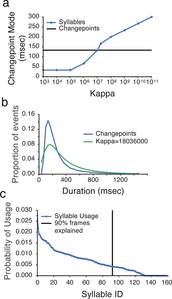
a. Scanning the MoSeq kappa parameter (which sets the timescale at which syllables are identified) reveals a value at which the modal syllable length matches the model-free block length identified by changepoints analysis (see Methods).

b. The mode of the syllable duration distribution established by MoSeq, given the kappa established in a, matches that for the model-free changepoint distribution.

c. Ninety percent of the total frames are explained by 92 behavioral syllables; for the sake of simplicity herein we analyze the top 90 syllables.

Extended Data Fig. 3.

A cladogram describing behavioral relationships among syllables was computed using hierarchical clustering performed on the autoregressive matrices describing all syllables (see Methods). Nine general behavioral categories were identified after visual inspection and given natural language names. Illustrations are representative of syllables in each category.

Extended Data Fig. 4.

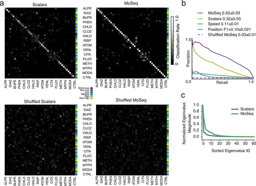
a. Normalized confusion matrices as in Fig. 3a, but computed for all drug/dose combinations. For the shuffled control (bottom row), syllable labels were shuffled on a per-mouse basis to compute a baseline of expected random performance. Heat map indicates classification successes and errors (see Methods for summary definitions).

b. Mean precision-recall curves for all drugs and doses, computed for each behavioral summary type.

c. The Fukunaga and Olsen method⁴⁴¹ was used to estimate the effective dimensionality of both scalar and MoSeq summaries; this analysis demonstrated that that MoSeq has a higher effective dimensionality than scalars (34 versus 26 dimensions), using a threshold value of 0.01 (see Methods).

Extended Data Fig. 5.

a. Additional information was added to the MoSeq and scalar behavioral summaries used to predict drug identity. For “MoSeq++,” the empirical transition matrix derived from the syllable label sequence was calculated, flattened, and concatenated to the syllable usage frequency information. For “Scalars++,” histograms of mouse acceleration, the mouse’s heading, the area contained by the mouse’s body contour, the ellipticity of the best-fit ellipse around the mouse’s contour, and the mouse’s width were added to the initial scalar behavioral summary.

b. The granularity of the bins used to generate scalar behavioral summaries was systematically varied; bin size did not affect classification performance.

c. To ensure that the higher dimensionality of the scalar summaries did not adversely affect performance, behavioral summaries containing scalars were also subjected to PCA to assess the consequences of dimensionality reduction (keeping the number of dimensions required to capture 95 percent of the variance; for scalars this is 33 dimensions); although performance was modestly improved, performance did not equal that observed for MoSeq.

Extended Data Fig. 6.

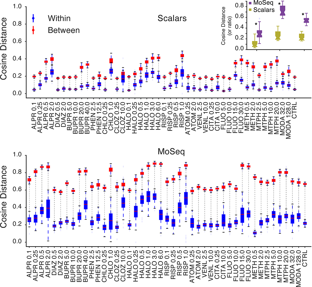
Average cosine distance ±1 standard deviation of mice given the same drug/dose pair (blue) and mice given different drug/dose pairs (red) using either scalar- (top) or MoSeq-based behavioral summaries (bottom). The difference observed between mice given the same drug/dose pair and different drug/dose pairs is uniformly larger when behavior is summarized using MoSeq when compared to scalars.

Inset: summary of mean within- and between- class differences and their ratio for either scalar- and MoSeq-based analysis. MoSeq shows larger differences (two-sided paired t-test, p<0.05, stars indicate statistically significant differences between MoSeq and scalars).

Extended Data Fig. 7.

To test whether the cosine distances that separate individual mice within a treatment class reflect individual variability or technical noise, we subsampled the data from each individual mouse and then asked how these sub-samples of each individual mouse compared to each other; observing low variability in these sub-samples would be consistent with each individual mouse expressing a stable set of behavioral syllables within an experiment, and with the within-condition variability observed across mice reflecting differences in individual mouse responses to a given drug and dose. In specific, within-mouse variability of MoSeq was assessed by randomly picking 1000 frames (with replacement) of the 3D imaging data (which for each mouse was constituted of approximately 36,000 frames), identifying the syllable associated by MoSeq with that frame, and then using those syllable labels to compute overall syllable usages; this procedure is roughly equivalent to randomly choosing less than one third of the syllables to quantify the pattern of syllable usage within a mouse. We repeated this procedure 100 times, and by computing cosine distances between each sub-sample within-mouse variability could be assessed. The bootstrapped estimate of individual variability (Resampled Within Mouse) was lower than the treatment-induced variability (Within tTreatment), as measured by the cosine distance between all pairs of mice given the same treatment, and was also lower than the cosine distance between pairs of mice given different treatments (Between Treatment). Thus the observed within-treatment variability reflects stable differences in behavior expressed by individual mice.

Extended Data Fig. 8.

a. Similar as Fig. 3a, but classifying drug/dose identity instead of drug identity, across the entire risperidone, haloperidol, clozapine dose-response experiment. Many significant syllables that differentiated drug-treated mice from controls were, by inspection, behaviors like grooming or rearing that do not include significant two-dimensional velocity components (data not shown).

b. Syllable usages for all mice and all drug/dose combinations (top), doses which resulted in slow mouse movement speed (middle) or moderate movement speed (bottom). Slow and medium speeds (relative to normal) were identified via a Gaussian Mixture Model (mean centroid speed of saline control mouse = 74 mm/sec; “medium speed” = 54 mm/sec; “slow speed” = 24 mm/sec; see Methods). Significant differential syllable usage for each drug versus control indicated with an asterisk (Kruskal-Wallis and post-hoc Dunn’s two-sided test with permutation, with Benjamini/Hochberg FDR with alpha = 0.05).

Extended Data Fig. 9.

Sparsification reveals the number of syllables required to correctly distinguish each drug, as assessed by F1 scores emerging from linear classifiers trained on subsets of syllables (see Methods).

References

- 1.Tinbergen N The study of instinct. (Clarendon Press, 1951). [Google Scholar]
- 2.Dawkins R in Growing points in ethology. (Cambridge U Press, 1976). [Google Scholar]
- 3.Datta SR, Anderson DJ, Branson K, Perona P & Leifer A Computational Neuroethology: A Call to Action. Neuron 104, 11–24, doi:papers3://publication/doi/ 10.1016/j.neuron.2019.09.038 (2019). [DOI] [PMC free article] [PubMed] [Google Scholar]
- 4.Anderson DJ & Perona P Toward a science of computational ethology. Neuron 84, 18–31, doi: 10.1016/j.neuron.2014.09.005 (2014). [DOI] [PubMed] [Google Scholar]
- 5.Mathis A et al. DeepLabCut: markerless pose estimation of user-defined body parts with deep learning. Nature Publishing Group 21, 1281–1289, doi:papers3://publication/doi/ 10.1038/s41593-018-0209-y (2018). [DOI] [PubMed] [Google Scholar]
- 6.Meyer AF, Poort J, O’Keefe J, Sahani M & Linden JF A Head-Mounted Camera System Integrates Detailed Behavioral Monitoring with Multichannel Electrophysiology in Freely Moving Mice. Neuron 100, 46–60.e47, doi:papers3://publication/doi/ 10.1016/j.neuron.2018.09.020 (2018). [DOI] [PMC free article] [PubMed] [Google Scholar]
- 7.Klaus A et al. The Spatiotemporal Organization of the Striatum Encodes Action Space. Neuron 95, 1171–1180.e1177, doi:papers3://publication/doi/ 10.1016/j.neuron.2017.08.015 (2017). [DOI] [PMC free article] [PubMed] [Google Scholar]
- 8.Pereira TD et al. Fast animal pose estimation using deep neural networks. Nature methods 16, 117–125, doi:papers3://publication/doi/ 10.1038/s41592-018-0234-5 (2019). [DOI] [PMC free article] [PubMed] [Google Scholar]
- 9.Wiltschko AB et al. Mapping sub-second structure in mouse behavior. Neuron 88, 1121–1135 (2015). [DOI] [PMC free article] [PubMed] [Google Scholar]
- 10.Graving JM et al. Fast and robust animal pose estimation. biorxiv.org, http:--dx.doi.org- 10.1101 - 620245, doi:papers3://publication/doi/ 10.1101/620245 (2019). [DOI] [PMC free article] [PubMed] [Google Scholar]
- 11.Markowitz JE et al. The Striatum Organizes 3D Behavior via Moment-to-Moment Action Selection. Cell 174, 44–58.e17 (2018). [DOI] [PMC free article] [PubMed] [Google Scholar]
- 12.Crawley JN Behavioral phenotyping of rodents. Comparative medicine 53, 140–146 (2003). [PubMed] [Google Scholar]
- 13.Crawley JN Behavioral phenotyping strategies for mutant mice. Neuron 57, 809–818, doi: 10.1016/j.neuron.2008.03.001 (2008). [DOI] [PubMed] [Google Scholar]
- 14.Crabbe JC Genetics of Mouse Behavior: Interactions with Laboratory Environment. Science (New York, NY) 284, 1670–1672, doi: 10.1126/science.284.5420.1670 (1999). [DOI] [PubMed] [Google Scholar]
- 15.Wahlsten D et al. Different data from different labs: Lessons from studies of gene-environment interaction. Journal of neurobiology 54, 283–311, doi: 10.1002/neu.10173 (2002). [DOI] [PubMed] [Google Scholar]
- 16.Egnor SER & Branson K Computational Analysis of Behavior. Annu. Rev. Neurosci. 39, 217–236 (2016). [DOI] [PubMed] [Google Scholar]
- 17.Berman GJ, Choi DM, Bialek W & Shaevitz JW Mapping the stereotyped behaviour of freely moving fruit flies. Journal of the Royal Society, Interface / the Royal Society 11, doi:papers3://publication/doi/ 10.1098/rsif.2014.0672 (2014). [DOI] [PMC free article] [PubMed] [Google Scholar]
- 18.Fentress JC & Stilwell FP Letter: Grammar of a movement sequence in inbred mice. Nature 244, 52–53 (1973). [DOI] [PubMed] [Google Scholar]
- 19.Berridge KC, Fentress JC & Parr H Natural syntax rules control action sequence of rats. Behavioural brain research 23, 59–68 (1987). [DOI] [PubMed] [Google Scholar]
- 20.Peñagarikano O et al. Absence of CNTNAP2 Leads to Epilepsy, Neuronal Migration Abnormalities, and Core Autism-Related Deficits. Cell 147, 235–246, doi: 10.1016/j.cell.2011.08.040 (2011). [DOI] [PMC free article] [PubMed] [Google Scholar]
- 21.Zetler G Haloperidol catalepsy in grouped and isolated mice. Pharmacology 13, 526–532, doi:papers3://publication/doi/ 10.1159/000136947 (1975). [DOI] [PubMed] [Google Scholar]
- 22.Millichap JG & Boldrey EE Studies in hyperkinetic behavior. II. Laboratory and clinical evaluations of drug treatments. Neurology 17, 467–471 (1967). [DOI] [PubMed] [Google Scholar]
- 23.Ebenezer I Neuropsychopharmacology and Therapeutics. (Wiley, 2015). [Google Scholar]
- 24.Duncan GE, Zorn S & Lieberman JA Mechanisms of typical and atypical antipsychotic drug action in relation to dopamine and NMDA receptor hypofunction hypotheses of schizophrenia. Molecular Psychiatry 4, 418–428, doi:papers3://publication/doi/ 10.1038/sj.mp.4000581 (1999). [DOI] [PubMed] [Google Scholar]
- 25.Roth BL, Sheffler DJ & Kroeze WK Magic shotguns versus magic bullets: selectively non-selective drugs for mood disorders and schizophrenia. Nat Rev Drug Discov 3, 353–359, doi:papers3://publication/doi/ 10.1038/nrd1346 (2004). [DOI] [PubMed] [Google Scholar]
- 26.McOmish CE, Lira A, Hanks JB & Gingrich JA Clozapine-induced locomotor suppression is mediated by 5-HT2A receptors in the forebrain. Neuropsychopharmacology : official publication of the American College of Neuropsychopharmacology 37, 2747–2755, doi:papers3://publication/doi/ 10.1038/npp.2012.139 (2012). [DOI] [PMC free article] [PubMed] [Google Scholar]
- 27.Volkow ND et al. Effects of modafinil on dopamine and dopamine transporters in the male human brain: clinical implications. JAMA 301, 1148–1154, doi:papers3://publication/doi/ 10.1001/jama.2009.351 (2009). [DOI] [PMC free article] [PubMed] [Google Scholar]
- 28.Zolkowska D et al. Evidence for the involvement of dopamine transporters in behavioral stimulant effects of modafinil. Journal of Pharmacology and Experimental Therapeutics 329, 738–746, doi:papers3://publication/doi/ 10.1124/jpet.108.146142 (2009). [DOI] [PMC free article] [PubMed] [Google Scholar]
- 29.Alarcón M et al. Linkage, association, and gene-expression analyses identify CNTNAP2 as an autism-susceptibility gene. Am. J. Hum. Genet. 82, 150–159, doi:papers3://publication/doi/ 10.1016/j.ajhg.2007.09.005 (2008). [DOI] [PMC free article] [PubMed] [Google Scholar]
- 30.Rodenas-Cuadrado P, Ho J & Vernes SC Shining a light on CNTNAP2: complex functions to complex disorders. Eur. J. Hum. Genet. 22, 171–178, doi:papers3://publication/doi/ 10.1038/ejhg.2013.100 (2014). [DOI] [PMC free article] [PubMed] [Google Scholar]
- 31.Brunner D et al. Comprehensive Analysis of the 16p11.2 Deletion and Null Cntnap2 Mouse Models of Autism Spectrum Disorder. PLoS ONE 10, e0134572–0134539, doi: 10.1371/journal.pone.0134572 (2015). [DOI] [PMC free article] [PubMed] [Google Scholar]
- 32.So H-C et al. Analysis of genome-wide association data highlights candidates for drug repositioning in psychiatry. Nature Neuroscience 20, 1342–1349, doi:papers3://publication/doi/ 10.1038/nn.4618 (2017). [DOI] [PubMed] [Google Scholar]
- 33.Ferreri F et al. The in Vitro Actions of Loxapine on Dopaminergic and Serotonergic Receptors. Time to Consider Atypical Classification of This Antipsychotic Drug? Int. J. Neuropsychopharmacol. 21, 355–360, doi:papers3://publication/doi/ 10.1093/ijnp/pyx102 (2018). [DOI] [PMC free article] [PubMed] [Google Scholar]
- 34.Datta SR Q&A: Understanding the composition of behavior. BMC biology 17, 44, doi:papers3://publication/doi/ 10.1186/s12915-019-0663-3 (2019). [DOI] [PMC free article] [PubMed] [Google Scholar]
- 35.Brown AEX, Yemini EI, Grundy LJ, Jucikas T & Schafer WR A dictionary of behavioral motifs reveals clusters of genes affecting Caenorhabditis elegans locomotion. Proceedings of the National Academy of Sciences 110, 791–796, doi: 10.1073/pnas.1211447110 (2013). [DOI] [PMC free article] [PubMed] [Google Scholar]
- 36.Berman GJ, Choi DM, Bialek W & Shaevitz JW Mapping the structure of drosophilid behavior. (2013).
- 37.Vogelstein JT et al. Discovery of brainwide neural-behavioral maps via multiscale unsupervised structure learning. Science (New York, NY) 344, 386–392, doi: 10.1126/science.1250298 (2014). [DOI] [PubMed] [Google Scholar]
- 38.Swinney DC & Anthony J How were new medicines discovered? Nat Rev Drug Discov 10, 507–519 (2011). [DOI] [PubMed] [Google Scholar]
- 39.Hendriksen H & Groenink L Back to the future of psychopharmacology: A perspective on animal models in drug discovery. Eur. J. Pharmacol. 759, 30–41 (2015). [DOI] [PubMed] [Google Scholar]
- 40.Witt PN Drugs alter web-building of spiders: a review and evaluation. Behav Sci 16, 98–113 (1971). [DOI] [PubMed] [Google Scholar]
Methods References
- 41.Fukunaga K & Olsen DR An algorithm for finding intrinsic dimensionality of data. IEEE Transactions on Computers 20, 176–183, doi:(null) (1971). [Google Scholar]
- 42.Bishop CM Pattern Recognition and Machine Learning. (Springer, 2006). [Google Scholar]
Associated Data
This section collects any data citations, data availability statements, or supplementary materials included in this article.
Supplementary Materials