

Abstract
Understanding how and why rates of character evolution vary across the Tree of Life is central to many evolutionary questions; for example, does the trophic apparatus (a set of continuous characters) evolve at a higher rate in fish lineages that dwell in reef versus nonreef habitats (a discrete character)? Existing approaches for inferring the relationship between a discrete character and rates of continuous-character evolution rely on comparing a null model (in which rates of continuous-character evolution are constant across lineages) to an alternative model (in which rates of continuous-character evolution depend on the state of the discrete character under consideration). However, these approaches are susceptible to a “straw-man” effect: the influence of the discrete character is inflated because the null model is extremely unrealistic. Here, we describe MuSSCRat, a Bayesian approach for inferring the impact of a discrete trait on rates of continuous-character evolution in the presence of alternative sources of rate variation (“background-rate variation”). We demonstrate by simulation that our method is able to reliably infer the degree of state-dependent rate variation, and show that ignoring background-rate variation leads to biased inferences regarding the degree of state-dependent rate variation in grunts (the fish group Haemulidae). [Bayesian phylogenetic comparative methods; continuous-character evolution; data augmentation; discrete-character evolution.]
Variable rates of continuous-character evolution are central to many evolutionary questions. These questions may involve changes in the rate of character evolution over time (time-dependent scenarios) or among lineages (lineage-specific scenarios). Such questions may be pursued by means of agnostic surveys to detect rate variation (data-exploration approaches; Harmon et al. 2010; Eastman et al. 2011; Venditti et al. 2011) or by testing predictions regarding factors hypothesized to influence rates of character evolution (hypothesis-testing approaches; O’Meara et al. 2006; Collar et al. 2009). A particular type of hypothesis posits that the rate of continuous-character evolution depends on the state of a discrete trait, for example, the evolutionary rate of the feeding apparatus (a set of continuous traits) in a lineage depends on the habitat type (the discrete trait) of its members.
Testing hypotheses regarding state-dependent rates of continuous-character evolution is currently pursued using a computational procedure (e.g., Collar et al. 2009, 2010; Price et al. 2011, 2013) comprised of four steps: 1) fit a Brownian motion model to the observations (the tree and continuous-trait values at its tips), where the rate of continuous-character evolution is assumed to be constant across all branches of the tree (the “null” or constant-rate model); 2) generate a sample of discrete-character histories (“stochastic maps”, Nielsen 2002; Huelsenbeck et al. 2003); 3) for each stochastic map, fit a Brownian motion model to the observations, where the instantaneous rate of continuous-character evolution at a given point on a given branch depends on the corresponding state of the discrete-character mapping (the “state-dependent model” O’Meara et al. 2006), and; 4) compare the fit of the state-dependent model (averaged over the sample of stochastic maps) to the constant-rate model using the Akaike Information Criterion (AIC). If the state-dependent model is preferred, we infer that rates of continuous-character evolution are correlated with the state of the discrete character.
The current approach has two potential problems. First, stochastic maps of the discrete character are generated without reference to the continuous characters. By construction, however, the state-dependent model specifies that the discrete and continuous characters are evolving jointly. The continuous characters therefore possess information about the history of the discrete character; disregarding this mutual information will lead to biased parameter estimates Revell 2012). Second, the null model—where the continuous characters are assumed to evolve at a constant rate across lineages—is extremely unrealistic. Any variation in the rate of continuous-character evolution—whether or not it is associated with the discrete character under consideration—is apt to be interpreted as evidence against the overly simplistic null model. This “straw-man effect” has the potential to mislead our inferences regarding the factors that impact rates of continuous-character evolution.
We describe a Bayesian approach for inferring the impact of a discrete trait on rates of continuous-character evolution that addresses the problems described above. We begin by developing a stochastic process that explicitly models the joint evolution of the discrete and continuous characters; this stochastic process can accommodate one or more continuous characters evolving under a state-dependent multivariate Brownian motion process. We refer to this new model as MuSSCRat (for Multiple State-Specific Rates of continuous-character evolution). We then develop an inference model that accommodates variation in the background rate of continuous-character evolution (i.e., rate variation across lineages that is independent of the discrete character under consideration). We implement this model in a Bayesian framework, which accommodates uncertainty in the phylogeny, discrete-character history, and parameters of the state-dependent model. We show by simulation that the method is able to reliably infer the state-dependent rates of continuous-character evolution, and that ignoring background-rate variation leads to an inflated false-positive rate. Finally, we demonstrate the new method with an empirical analysis of grunts (a group of haemulid fish) to illustrate the impacts of background-rate variation and prior specification on inferences about state-dependent rate variation.
Methods
Our goal is to develop a state-dependent multivariate Brownian motion model, MuSSCRat, in a Bayesian statistical framework. We begin with a simple simulation to describe the parameters and basic properties of the MuSSCRat model. We then show how to calculate the probability of observing the discrete and continuous characters across the tips of a phylogeny under the model (i.e., how to compute the likelihood). Finally, we describe the relevant details—the priors and Markov chain Monte Carlo (MCMC) machinery—required to perform Bayesian inference under the MuSSCRat model.
The State-Dependent Multivariate Brownian Motion Process
A simulation example
We introduce the salient properties of the MuSSCRat model by
describing a simple simulation with a binary discrete character,
 , and a single continuous character,
 , over a single branch. The discrete
character has two states, 0 and 1; the continuous character can be any real number. The
state of the simulation at time
, over a single branch. The discrete
character has two states, 0 and 1; the continuous character can be any real number. The
state of the simulation at time  is the pair of
discrete- and continuous-character values,
is the pair of
discrete- and continuous-character values,  . (We use
capital letters—
. (We use
capital letters— and
and  —to
represent random variables, and lowercase letters—
—to
represent random variables, and lowercase letters— and
and
 —to represent specific values of those
random variables.)
—to represent specific values of those
random variables.)
The discrete trait evolves under a continuous-time Markov process, changing from state
0 to state 1 with rate  , and from state 1 to state 0 with
rate
, and from state 1 to state 0 with
rate  . The continuous character evolves
under a state-dependent Brownian motion process, where the diffusion rate,
. The continuous character evolves
under a state-dependent Brownian motion process, where the diffusion rate,
 , measures the rate of
continuous-character evolution when the discrete character is in state
, measures the rate of
continuous-character evolution when the discrete character is in state
 (i.e.,
  indicates that the continuous
character evolves faster in discrete state 1 than in discrete state 0). In a small time
interval of duration
indicates that the continuous
character evolves faster in discrete state 1 than in discrete state 0). In a small time
interval of duration  , where the discrete character
begins in state
, where the discrete character
begins in state  , the continuous character changes by a
normally distributed random variable with mean 0 and variance
, the continuous character changes by a
normally distributed random variable with mean 0 and variance  , and the discrete character
changes state with probability
, and the discrete character
changes state with probability  .
.
We begin the simulation at time  , with the
discrete character in state
, with the
discrete character in state  and the continuous character with
value
and the continuous character with
value  . We then increment the simulation
forward in time by a small time interval,
. We then increment the simulation
forward in time by a small time interval,  , applying the
above rules describing how the state of the process changes during each time interval.
We continue to increment the simulation forward in time until we reach the end of the
branch (at time
, applying the
above rules describing how the state of the process changes during each time interval.
We continue to increment the simulation forward in time until we reach the end of the
branch (at time  ). The outcome of the simulation is a
sample path that records the state of the process from the beginning
to the end of the branch (Fig. 1a).
). The outcome of the simulation is a
sample path that records the state of the process from the beginning
to the end of the branch (Fig. 1a).
Figure 1.

Simulations under the state-dependent multivariate Brownian motion process. The
process is either in discrete state 0 (blue) or discrete state 1 (orange), where the
rate of change between discrete states is equal ( ), and the rate of
continuous-character evolution is higher when the process is in the orange state
(
), and the rate of
continuous-character evolution is higher when the process is in the orange state
( ,
,
 ). A) A single sample path
from
). A) A single sample path
from  to
to  . The process begins and ends in the
blue state, but spends some time in the orange state. Note that there is more
evolution in the orange state than in the blue state. B) The distribution of end
states for 10 million simulated realizations. Solid lines represent the simulated
joint probability densities of the discrete and continuous states. Dashed lines
represent the normal densities with parameters estimated from the simulated end
states. Note that the simulated densities depart from the normal densities (both
Kolmogorov–Smirnov
. The process begins and ends in the
blue state, but spends some time in the orange state. Note that there is more
evolution in the orange state than in the blue state. B) The distribution of end
states for 10 million simulated realizations. Solid lines represent the simulated
joint probability densities of the discrete and continuous states. Dashed lines
represent the normal densities with parameters estimated from the simulated end
states. Note that the simulated densities depart from the normal densities (both
Kolmogorov–Smirnov 
The transition-probability density specifies the probability that the
process ends in some state,  , given an initial state
 , after a certain amount of
time,
, after a certain amount of
time,  , has elapsed. The resulting frequency
histogram of end states provides a Monte Carlo approximation of the
transition-probability density for a branch of duration
, has elapsed. The resulting frequency
histogram of end states provides a Monte Carlo approximation of the
transition-probability density for a branch of duration
 . Note that the transition-probability
densities of standard (i.e., state-independent) Brownian motion processes are normal
densities. By contrast, it is clear from our simulations that the transition-probability
densities under the state-dependent process are not normal densities (Fig. 1b).
. Note that the transition-probability
densities of standard (i.e., state-independent) Brownian motion processes are normal
densities. By contrast, it is clear from our simulations that the transition-probability
densities under the state-dependent process are not normal densities (Fig. 1b).
Parameters of the MuSSCRat model
We model the joint evolution of a discrete binary character,  , and
a set of
, and
a set of  continuous characters,
 , as a stochastic process.
The discrete trait has two possible values, which we arbitrarily label
, as a stochastic process.
The discrete trait has two possible values, which we arbitrarily label
 and
and  ;
;
 . The continuous characters
are a vector of real-valued random variables, where
. The continuous characters
are a vector of real-valued random variables, where  is
the value of the
is
the value of the  continuous character
(
continuous character
( ).
Variables of the MuSSCRat model are summarized in Table 1.
).
Variables of the MuSSCRat model are summarized in Table 1.
Table 1.
The variables of the MuSSCRat model and their interpretation.
| Variable | Interpretation |
|---|---|

|
The continuous characters for one lineage |

|
The state of the continuous characters at time

|

|
The number of continuous characters |

|
An  matrix containing the matrix containing the
 continuous characters for the continuous characters for the
 species in the tree species in the tree |

|
The discrete character for one lineage |

|
The state of the discrete character at time

|

|
An  matrix containing the
discrete character for the matrix containing the
discrete character for the  species in the
tree species in the
tree |

|
The complete history of the discrete character (the state at the beginning and end of the process, |
and all of the changes in between) along the lineage

|
|

|
The instantaneous-rate matrix of the discrete-character CTMC model |

|
The instantaneous rate of change from state
 to state to state

|

|
The background rate of continuous-character evolution among all lineages |

|
The background rate of continuous-character evolution for lineage

|

|
The relative rates of continuous-character evolution for each continuous character |

|
The relative rates of continuous-character evolution for each discrete state |

|
The evolutionary correlation matrix |

|
The evolutionary correlation between continuous characters
 and and 
|

|
The discrete-state-independent evolutionary variance–covariance matrix |
We assume that the discrete character evolves under a continuous-time Markov process,
and that the continuous characters evolve under a multivariate Brownian motion process
with rates that depend on the state of the binary character. These model components
collectively describe how the set of characters,  , evolve together over a
single branch; we detail the evolutionary dynamics of this process over an entire tree
when we describe the likelihood function.
, evolve together over a
single branch; we detail the evolutionary dynamics of this process over an entire tree
when we describe the likelihood function.
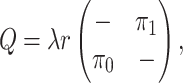
The instantaneous-rate matrix,  , describes the rates
at which the binary character evolves:
, describes the rates
at which the binary character evolves:  describes the
instantaneous rate of change from state
describes the
instantaneous rate of change from state  to state
 :
:
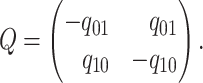 |
The complete history of the discrete trait on branch  —which
we represent as
—which
we represent as  —specifies the state of the
character at the beginning and end of the branch, and also the times of any state
changes along the branch.
—specifies the state of the
character at the beginning and end of the branch, and also the times of any state
changes along the branch.
While the process is in a particular discrete state, we assume the continuous
characters evolve under a multivariate Brownian motion model. We allow the background
rate of evolution to vary among lineages in the phylogeny by letting each branch have
its own rate parameter,  (we call this “background-rate
variation”). While in discrete state
(we call this “background-rate
variation”). While in discrete state  , the background rate
is multiplied by the state-specific relative rate,
, the background rate
is multiplied by the state-specific relative rate,  . We also allow the relative rate
of evolution to vary among the continuous characters. The vector
. We also allow the relative rate
of evolution to vary among the continuous characters. The vector
 contains these
relative rates;
contains these
relative rates;  is the relative rate at which
continuous character
is the relative rate at which
continuous character  evolves. The evolutionary correlations
between characters are contained in the
evolves. The evolutionary correlations
between characters are contained in the  symmetric
correlation matrix,
symmetric
correlation matrix,  , where
  specifies the
correlation between characters
specifies the
correlation between characters  and
and
 .
.
We assume that the relative rates of change between characters,
 , and the
evolutionary correlations between characters,
, and the
evolutionary correlations between characters,  , are independent of
the discrete state; in other words, we assume that the state of the discrete trait
affects only the overall rate of continuous-character evolution, but
not the nature of the evolutionary process (as represented by
, are independent of
the discrete state; in other words, we assume that the state of the discrete trait
affects only the overall rate of continuous-character evolution, but
not the nature of the evolutionary process (as represented by
 and
and
 ). We combine the relative rates among
characters and the correlation matrix to form the overall evolutionary
variance-covariance matrix,
). We combine the relative rates among
characters and the correlation matrix to form the overall evolutionary
variance-covariance matrix,  :
:
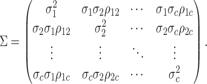 |
Bayesian Inference
We implement the MuSSCRat model with background-rate variation as a Bayesian model to infer the joint posterior density of the parameters given the observed data. We must specify both the likelihood function and also the joint prior density to compute the joint posterior distribution. We describe each of these components below.
Data
We imagine that we have sampled one discrete character and  continuous characters for each of
  species; relationships
among these species are defined by the phylogeny,
species; relationships
among these species are defined by the phylogeny,  .
We store the discrete characters in an
.
We store the discrete characters in an  column
vector,
column
vector,  , and the continuous
characters in an
, and the continuous
characters in an  matrix,
 . We assume that the discrete
and continuous characters evolve independently along each of the
. We assume that the discrete
and continuous characters evolve independently along each of the
 branches of the tree. We index the
internal nodes according to their sequence in a post-order traversal of the tree,
starting from the root (which has index
branches of the tree. We index the
internal nodes according to their sequence in a post-order traversal of the tree,
starting from the root (which has index  ).
).
Likelihood function
We simplify likelihood calculations by including the vector of character histories,
 , where
 is the discrete-character
history along branch
is the discrete-character
history along branch  (including the state at the beginning
and end of the branch), as variables in the model. In effect, we are “augmenting” the
discrete-character data observed at the tips of the tree with unobserved
discrete-character histories over the entire tree; this technique is referred to as
data augmentation (Tanner and Wong
1987; Robinson et al. 2003; Mateiu and Rannala 2006; Lartillot 2006; Landis et al.
2013).
(including the state at the beginning
and end of the branch), as variables in the model. In effect, we are “augmenting” the
discrete-character data observed at the tips of the tree with unobserved
discrete-character histories over the entire tree; this technique is referred to as
data augmentation (Tanner and Wong
1987; Robinson et al. 2003; Mateiu and Rannala 2006; Lartillot 2006; Landis et al.
2013).
The augmented likelihood is a product of the joint probability of
 and
the conditional probability density of
and
the conditional probability density of  given
given
 :
:
 |
where  are the parameters of the
MuSSCRat model. We compute the joint probability of
are the parameters of the
MuSSCRat model. We compute the joint probability of
 as a
product of independent probabilities across each of the
as a
product of independent probabilities across each of the  branches:
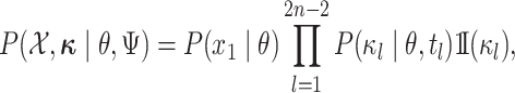 |
where  is
an indicator function that ensures that character histories are consistent across
ancestor-descendant branches (i.e., that the state at the end of one branch matches the
state at the beginning of its descendant branches), and ensures that character histories
for terminal branches end in the observed state. We compute
is
an indicator function that ensures that character histories are consistent across
ancestor-descendant branches (i.e., that the state at the end of one branch matches the
state at the beginning of its descendant branches), and ensures that character histories
for terminal branches end in the observed state. We compute  as
illustrated in Figure 2. By convention, we use the
stationary distribution of the Markov chain defined by
as
illustrated in Figure 2. By convention, we use the
stationary distribution of the Markov chain defined by  as
the probability of the root state,
as
the probability of the root state,  .
.
Figure 2.
Computing the probability of a character history,  . Blue and orange segments
correspond to discrete states 0 and 1, respectively. The probability of the history
is the product of the probabilities of waiting times between events (or the
probability of no event in the final segment) given the current rate of change.
. Blue and orange segments
correspond to discrete states 0 and 1, respectively. The probability of the history
is the product of the probabilities of waiting times between events (or the
probability of no event in the final segment) given the current rate of change.
To calculate the conditional probability density of the continuous characters, we first
consider how the continuous characters,  , evolve
along a single branch of length
, evolve
along a single branch of length  when the history of
the discrete character along that branch is known. Given that the discrete character is
in state
when the history of
the discrete character along that branch is known. Given that the discrete character is
in state  for duration
  ,
changes in the continuous character follow a multivariate normal distribution with mean
,
changes in the continuous character follow a multivariate normal distribution with mean
 and variance-covariance
matrix
and variance-covariance
matrix  .
This implies that the changes in
.
This implies that the changes in  while in
discrete state
while in
discrete state  ,
,  , are
multivariate-normally distributed:
, are
multivariate-normally distributed:
 |
where  is the amount of time
the history spends in discrete state
is the amount of time
the history spends in discrete state  and
and
 is a
is a
 vector of zeros (indicating
that the expected amount of change for each continuous character is 0). Because it is
the sum of multivariate-normally distributed random variables,
vector of zeros (indicating
that the expected amount of change for each continuous character is 0). Because it is
the sum of multivariate-normally distributed random variables,  is also multivariate-normally distributed:
 |
where  is the branch-specific variance-covariance matrix given the discrete-character history
and the background rate of evolution for the branch,
is the branch-specific variance-covariance matrix given the discrete-character history
and the background rate of evolution for the branch,  .
.
Because changes to the continuous characters follow a multivariate normal distribution,
we can compute the conditional probability density of the continuous characters,
 ,
using standard algorithms to integrate over the distributions of the states at internal
nodes. Specifically, we use Felsenstein’s REML algorithm (Felsenstein 1973, 2004), extended to
multivariate Brownian motion (Huelsenbeck and Rannala
2003; Freckleton 2012), to compute the
conditional probability density of
,
using standard algorithms to integrate over the distributions of the states at internal
nodes. Specifically, we use Felsenstein’s REML algorithm (Felsenstein 1973, 2004), extended to
multivariate Brownian motion (Huelsenbeck and Rannala
2003; Freckleton 2012), to compute the
conditional probability density of  . This
algorithm assumes a uniform prior over all possible continuous states at the root.
. This
algorithm assumes a uniform prior over all possible continuous states at the root.
Incorporating background-rate variation in the MuSSCRat model does not complicate the computation of the augmented likelihood, since it simply “rescales” the variance-covariance matrices on each branch. However, including background-rate variation does complicate inference; specifically, it causes the MuSSCRat model to become nonidentifiable (see Supplementary Material available on Dryad at http://dx.doi.org/10.5061/dryad.499c4j2). A model is nonidentifiable when multiple combinations of parameters have identical likelihoods (Rannala 2002). Consequently, parameters of a nonidentifiable model cannot be estimated by standard maximum-likelihood methods because there may be no unique “maximum” likelihood. In this case, it is necessary to apply constraints on nonidentifiable parameters that “penalize” different combinations of parameters that have identical likelihoods. Bayesian models provide a natural solution to nonidentifiability, as the prior distributions on the parameters naturally penalize combinations of parameters that might have identical likelihoods (i.e., the joint posterior probability of parameter combinations with identical likelihoods will differ if their joint prior probabilities are different). We describe our assumed prior distribution on background rates in the next section.
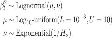
Priors
We assume that the background-rate parameters,  , are drawn from a
hierarchical model with parameters
, are drawn from a
hierarchical model with parameters  and
and
 , and the remainder of the parameters
are drawn from independent prior distributions, so that the joint prior density becomes:
, and the remainder of the parameters
are drawn from independent prior distributions, so that the joint prior density becomes:
 |
We describe our prior distributions in the following paragraphs; these parameterizations reflect our “baseline” model, but we explore alternative priors and prior sensitivity in our empirical analyses.
We draw the lineage-specific background rates of continuous-character evolution,
 , iid from a shared
lognormal distribution with mean
, iid from a shared
lognormal distribution with mean  and standard
deviation
and standard
deviation  . We use a uniform prior on
 , such that
 is drawn from a
log
is drawn from a
log -uniform distribution between
 and
and  . We
draw the standard deviation,
. We
draw the standard deviation,  , from an
exponential distribution with mean
, from an
exponential distribution with mean  . The constant
 is the standard deviation for a
lognormal distribution that indicates that our
is the standard deviation for a
lognormal distribution that indicates that our  prior belief ranges over one order of magnitude (see Supplementary Material available on
Dryad). This model is the continuous-character analog of the uncorrelated lognormal
(UCLN) relaxed-clock model used to describe variation in rates of molecular evolution
across lineages (e.g., Drummond et al. 2006; Lemey et al. 2010). Accordingly, we refer to this
extension of the MuSSCRat model with background-rate variation as
the MuSSCRat + UCLN model. A convenient property of the UCLN
model is that—as
prior belief ranges over one order of magnitude (see Supplementary Material available on
Dryad). This model is the continuous-character analog of the uncorrelated lognormal
(UCLN) relaxed-clock model used to describe variation in rates of molecular evolution
across lineages (e.g., Drummond et al. 2006; Lemey et al. 2010). Accordingly, we refer to this
extension of the MuSSCRat model with background-rate variation as
the MuSSCRat + UCLN model. A convenient property of the UCLN
model is that—as  shrinks to 0—it collapses to a
“strict” morphological-clock model, where
shrinks to 0—it collapses to a
“strict” morphological-clock model, where  for all
lineages. Our prior on
for all
lineages. Our prior on  specifies that we expect the values
of
specifies that we expect the values
of  to range over about
one order of magnitude, but the exponential prior allows the standard deviation to
shrink to 0 if the data prefer a strict morphological clock. In summary, we specify the
background-rate-variation component of the prior model as:
to range over about
one order of magnitude, but the exponential prior allows the standard deviation to
shrink to 0 if the data prefer a strict morphological clock. In summary, we specify the
background-rate-variation component of the prior model as:
 |
The parameter vector  describes the
relative rate of continuous-character evolution for each of the discrete states. We
specify a Dirichlet distribution on half the values of
describes the
relative rate of continuous-character evolution for each of the discrete states. We
specify a Dirichlet distribution on half the values of
 . Specifying the
prior on half the values of
. Specifying the
prior on half the values of  ensures that the mean value of
  is
1, which allows us to interpret these parameters as the relative rate
of continuous-character evolution in the alternative discrete states. We assume the
concentration parameters of the Dirichlet distribution are the same, so this is a
symmetric Dirichlet distribution with parameter
is
1, which allows us to interpret these parameters as the relative rate
of continuous-character evolution in the alternative discrete states. We assume the
concentration parameters of the Dirichlet distribution are the same, so this is a
symmetric Dirichlet distribution with parameter  :
:
 |
The average rate of change for each of the  continuous characters
may vary; we allow the relative rate of continuous characters to vary by including a
parameter vector,
continuous characters
may vary; we allow the relative rate of continuous characters to vary by including a
parameter vector,  , where
 is the rate of evolution of
the
is the rate of evolution of
the  continuous character. We
specify a Dirichlet distribution on
continuous character. We
specify a Dirichlet distribution on  of the
values of
of the
values of  . We adopt the same
logic as above for the prior on
. We adopt the same
logic as above for the prior on  ,
specifying a symmetric Dirichlet distribution with parameter
,
specifying a symmetric Dirichlet distribution with parameter  such that the mean value of
 is 1:
is 1:
 |
The symmetric matrix  determines the evolutionary correlation
between each pair of continuous characters;
determines the evolutionary correlation
between each pair of continuous characters;  is the correlation between characters
  and
and
 . The matrix
  has
a special constraint (it must be positive semidefinite) that makes it difficult to
specify, for example, iid priors on each matrix element,
has
a special constraint (it must be positive semidefinite) that makes it difficult to
specify, for example, iid priors on each matrix element,  . We use the LKJ distribution as a
prior on
. We use the LKJ distribution as a
prior on  , which defines a prior over
positive-semidefinite correlation matrices (Lewandowski
et al. 2009). Correlation matrices drawn from this distribution have prior
density:
, which defines a prior over
positive-semidefinite correlation matrices (Lewandowski
et al. 2009). Correlation matrices drawn from this distribution have prior
density:
 |
where  is inversely related to the
variance of the correlation parameters: larger values of
is inversely related to the
variance of the correlation parameters: larger values of  result in marginal distributions on
  that are
concentrated closer to 0, while smaller values of
that are
concentrated closer to 0, while smaller values of  result in distributions that are more diffuse. We choose
  , which indicates a uniform
distribution over all possible positive-semidefinite correlation matrices:
, which indicates a uniform
distribution over all possible positive-semidefinite correlation matrices:
 |
Finally, the matrix  describes the rates of change between
the discrete-character states. We parameterize the stationary frequencies,
describes the rates of change between
the discrete-character states. We parameterize the stationary frequencies,
 , and the average rate of
change,
, and the average rate of
change,  . We build
 from these parameters as follows:
 |
where the diagonal elements are specified so that the sum of each row is 0, and the
scalar  is an arbitrary value that guarantees
that the expected number of transitions over a tree of length
is an arbitrary value that guarantees
that the expected number of transitions over a tree of length  is
is
 .
.
Assuming that the rates of change are symmetric ( ) or asymmetric
(
) or asymmetric
( ) may have some impact
on our analysis through the distribution on
) may have some impact
on our analysis through the distribution on  .
Moreover, inferring whether rates of change are (a)symmetric is often of direct interest
to researchers studying discrete-character evolution. We therefore specify a mixture
distribution on
.
Moreover, inferring whether rates of change are (a)symmetric is often of direct interest
to researchers studying discrete-character evolution. We therefore specify a mixture
distribution on  , so that
 may be symmetric or
asymmetric. Specifically, we draw
may be symmetric or
asymmetric. Specifically, we draw  , from
a degenerate distribution concentrated on equal rates,
, from
a degenerate distribution concentrated on equal rates,  , with
probability
, with
probability  , and from a Dirichlet
distribution with parameter
, and from a Dirichlet
distribution with parameter  with
probability
with
probability  . We draw
 from a lognormal prior
distribution with standard deviation
from a lognormal prior
distribution with standard deviation  , and specify the mean
such that the expected number of transitions over the entire phylogeny is
, and specify the mean
such that the expected number of transitions over the entire phylogeny is
 . The prior expected number of
transitions reflects an empirical prior, and should be specified differently for
different data sets; for the simulations and analyses we describe later, we use
. The prior expected number of
transitions reflects an empirical prior, and should be specified differently for
different data sets; for the simulations and analyses we describe later, we use
 . Our overall prior on
 is:
is:
 |
Posterior
Having specified the augmented likelihood function and the joint prior density, we can write down the joint posterior density of the model parameters and the discrete-character histories:
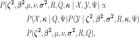 |
(1) |
where the first two terms on the right-hand side are the augmented likelihood, and the third term is the joint prior density on the model parameters.
The above Bayesian model conditions on a known tree,  .
It is straightforward to relax the assumption of a fixed tree by including it as a
parameter in the model. In this case, we may include a sequence alignment and specify a
subsitution model, and jointly infer the phylogeny and the parameters of the
MuSSCRat and substitution models.
.
It is straightforward to relax the assumption of a fixed tree by including it as a
parameter in the model. In this case, we may include a sequence alignment and specify a
subsitution model, and jointly infer the phylogeny and the parameters of the
MuSSCRat and substitution models.
Constant background rates
The MuSSCRat model with constant-background rates is nested
within the model with background-rate variation described above: as
 , the lognormal prior on
 collapses to a point
centered on
collapses to a point
centered on  (so that all values of
 for all branches
become increasingly similar).
for all branches
become increasingly similar).
To specify the constant-background-rate model explicitly, we draw a single value for
 from a
log
from a
log -uniform distribution between
 and
and  .
Otherwise, we use the same prior distributions for the constant-background-rate model as
we described for the variable-background-rate model, above.
.
Otherwise, we use the same prior distributions for the constant-background-rate model as
we described for the variable-background-rate model, above.
Markov chain Monte Carlo
The joint posterior probability density cannot be calculated analytically because we
cannot evaluate the normalizing constant of equation 1 (the marginal likelihood). We therefore approximate the joint
posterior probability density numerically using MCMC; specifically, we draw samples from
the joint posterior distribution using the Metropolis–Hastings and Green algorithm
(Metropolis et al. 1953; Hastings 1970; Green 1995). We
use standard proposal distributions for the majority of the model parameters; for
brevity, we only provide details for two of our more uncommon proposal distributions—for
moves between symmetric and asymmetric  matrices, and for the
discrete-character histories—in the Supplementary Material available on Dryad.
matrices, and for the
discrete-character histories—in the Supplementary Material available on Dryad.
Our data-augmentation strategy involves including the complete history of the discrete
character,  , as a variable in the
Markov chain. As such, the MCMC procedure includes proposals that change the
discrete-character history. When a new character history,
, as a variable in the
Markov chain. As such, the MCMC procedure includes proposals that change the
discrete-character history. When a new character history,  , is proposed, it is
accepted with probability
, is proposed, it is
accepted with probability  , computed as:
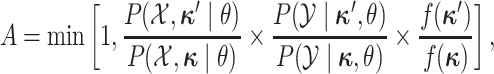 |
where  is the
distribution from which the new character history is drawn. Note that the probabilities
of the discrete characters,
is the
distribution from which the new character history is drawn. Note that the probabilities
of the discrete characters,  ,
and continuous characters,
,
and continuous characters,  ,
both contribute to the probability that the proposed discrete-character history is
accepted. Importantly, this means that the continuous characters are able to correctly
influence the discrete-character histories; that is, we are correctly modeling the joint
distribution of the discrete and continuous characters.
,
both contribute to the probability that the proposed discrete-character history is
accepted. Importantly, this means that the continuous characters are able to correctly
influence the discrete-character histories; that is, we are correctly modeling the joint
distribution of the discrete and continuous characters.
Implementation
We implemented our MuSSCRat model in the open-source Bayesian phylogenetic software, RevBayes (Höhna et al. 2016). Our implementation relies upon the data-augmentation functionality developed in RevBayes by Michael J. Landis and Sebastian Höhna for discrete characters (unpublished), extended to accommodate phylogenetic uncertainty. Owing to the flexibility of RevBayes, our implementation allows users to explore the impact of binary or multistate discrete traits on rates of continuous-character evolution, provides tremendous flexibility for specifying priors, enables simultaneous inference of ancestral states for both discrete and continuous characters, and allows joint inference of the phylogeny, divergence times, and parameters of the MuSSCRat model. We provide Rev scripts for performing analyses under the MuSSCRat model in RevBayes (see Data Dryad repository http://doi.org/10.5061/dryad.499c4j2 and GitHub repository https://github.com/mikeryanmay/musscrat_supp_archive/releases/tag/1.1.
Statistical behavior
The MuSSCRat model has many parameters relative to the number of
observations,  and
and  . It is therefore unclear how well
this complex model can detect rate variation, or distinguish between state-dependent and
background sources of rate variation. Accordingly, we performed a simulation study to
characterize the statistical behavior of the state-dependent model. Specifically, we
performed experiments to understand: 1) its ability to detect state-dependent rate variation
in the absence of background-rate variation; 2) its ability to detect state-dependent rate
variation in the presence of background-rate variation; 3) the cost of including
background-rate variation in the model when background rates are actually constant, and; 4)
the consequences of assuming background rates are constant when they are actually
variable.
. It is therefore unclear how well
this complex model can detect rate variation, or distinguish between state-dependent and
background sources of rate variation. Accordingly, we performed a simulation study to
characterize the statistical behavior of the state-dependent model. Specifically, we
performed experiments to understand: 1) its ability to detect state-dependent rate variation
in the absence of background-rate variation; 2) its ability to detect state-dependent rate
variation in the presence of background-rate variation; 3) the cost of including
background-rate variation in the model when background rates are actually constant, and; 4)
the consequences of assuming background rates are constant when they are actually
variable.
For the following analyses, we approximated the joint posterior probability density by running two replicate MCMC simulations for each simulated data set. We performed MCMC diagnosis to ensure that the joint posterior density was adequately approximated. We provide details of the MCMC simulations and MCMC diagnoses in the Supplementary Material available on Dryad.
Measures of Performance
Frequentist properties
The frequentist interpretation of a Bayesian credible interval (CI) is that the true
value of a parameter has a  chance of being
within the
chance of being
within the  CI of its
corresponding marginal posterior distribution (assuming the model is true, see Huelsenbeck and Rannala 2004). With this
interpretation in mind, we assessed the frequentist properties of the
CI of its
corresponding marginal posterior distribution (assuming the model is true, see Huelsenbeck and Rannala 2004). With this
interpretation in mind, we assessed the frequentist properties of the
 CI inferred for our simulated data
sets (assuming the conventional significance level,
CI inferred for our simulated data
sets (assuming the conventional significance level,  ). We define the
coverage probability as the frequency with which the true value of a
parameter is contained in the
). We define the
coverage probability as the frequency with which the true value of a
parameter is contained in the  CI, the
false-positive rate as the frequency with which the true value is
excluded from the
CI, the
false-positive rate as the frequency with which the true value is
excluded from the  CI (one minus the coverage
probability), and the power as the frequency with which a
state-independent model is excluded from the
CI (one minus the coverage
probability), and the power as the frequency with which a
state-independent model is excluded from the  CI when the
state-dependent model is true.
CI when the
state-dependent model is true.
Accuracy and bias
We assess the accuracy and bias of the posterior-mean estimate of
 using the percent-error
statistic, defined as:
using the percent-error
statistic, defined as:
 |
where  is the true value of
state-dependent rate for discrete state 1, and
is the true value of
state-dependent rate for discrete state 1, and  is estimated value of
the state-dependent rate for discrete state 1 (we use the mean of the corresponding
marginal posterior distribution). Values of
is estimated value of
the state-dependent rate for discrete state 1 (we use the mean of the corresponding
marginal posterior distribution). Values of  indicate an underestimate; conversely, values of
  indicate an
overestimate.
indicate an
overestimate.
Simulation Experiments
Experiment 1: Constant background rates
We simulated data sets of different sizes (with  continuous
characters), over a variety of tree sizes (with
continuous
characters), over a variety of tree sizes (with  species), and
state-dependent rate-ratios,
species), and
state-dependent rate-ratios,  (where
  corresponds
to the case when rates do not depend on the state of the discrete trait). For each
combination of
corresponds
to the case when rates do not depend on the state of the discrete trait). For each
combination of  ,
,  , and
, and
 , we simulated 100
trees under a constant-rate birth–death process with a speciation rate of 1 and an
extinction rate of 0.5 using the R (R Core Team 2017) package TESS (Höhna et al. 2015); we then rescaled each tree to
have a root height of 1. We simulated discrete-character histories under a symmetric
continuous-time Markov chain with a rate specified such that the expected number of
transitions was 5. We then drew correlation matrices from an LKJ distribution with
, we simulated 100
trees under a constant-rate birth–death process with a speciation rate of 1 and an
extinction rate of 0.5 using the R (R Core Team 2017) package TESS (Höhna et al. 2015); we then rescaled each tree to
have a root height of 1. We simulated discrete-character histories under a symmetric
continuous-time Markov chain with a rate specified such that the expected number of
transitions was 5. We then drew correlation matrices from an LKJ distribution with
 , and relative rates for each
continuous character from a symmetric Dirichlet distribution with
, and relative rates for each
continuous character from a symmetric Dirichlet distribution with
 . Finally, we simulated
 continuous characters under a
multivariate Brownian motion model assuming a background rate of 1. We provide more
details for the simulation procedure in the Supplementary Material available on
Dryad.
continuous characters under a
multivariate Brownian motion model assuming a background rate of 1. We provide more
details for the simulation procedure in the Supplementary Material available on
Dryad.
We analyzed each simulated data set in RevBayes under the
MuSSCRat model, assuming the true phylogeny was known. We
constrained the model so that the background rate was equal for each lineage (i.e., the
constant-rate model), and excluded the standard deviation parameter,
 , from the model. We estimated the
remaining model parameters from the simulated data using the priors described in the
Bayesian inference section, above. Since the generating model and the inference model
both exclude background-rate variation, this simulation scenario reflects the
performance of the method when the model is correctly specified.
, from the model. We estimated the
remaining model parameters from the simulated data using the priors described in the
Bayesian inference section, above. Since the generating model and the inference model
both exclude background-rate variation, this simulation scenario reflects the
performance of the method when the model is correctly specified.
The false-positive rate for this simulation experiment was  (i.e., when
  ; Fig. 3, the top row of the top three panels), which is
indistinguishable from the expected
; Fig. 3, the top row of the top three panels), which is
indistinguishable from the expected  (two-tailed
binomial test
(two-tailed
binomial test  ,
,
 ). Next, we
computed the power when rates of continuous-character evolution varied among discrete
states (
). Next, we
computed the power when rates of continuous-character evolution varied among discrete
states ( ). The power
ranged from
). The power
ranged from  to
to
 from the worst-case to the
best-case scenarios. Predictably, power improved as the number of continuous characters
and species increased; overall, the average power was
from the worst-case to the
best-case scenarios. Predictably, power improved as the number of continuous characters
and species increased; overall, the average power was  (Fig. 3, top three panels, excluding the top
row). The posterior-mean estimate of
(Fig. 3, top three panels, excluding the top
row). The posterior-mean estimate of  was slightly
biased for small numbers of continuous characters (
was slightly
biased for small numbers of continuous characters ( ) but quickly converged to the
true value as the number of characters and species increased (Fig. 4, top row of panels).
) but quickly converged to the
true value as the number of characters and species increased (Fig. 4, top row of panels).
Figure 3.

The frequency with which  was
excluded from the
was
excluded from the  CI when background rates were
constant (top row of panels) or variable (bottom row of panels). Each panel
corresponds to simulations for a given number of species,
CI when background rates were
constant (top row of panels) or variable (bottom row of panels). Each panel
corresponds to simulations for a given number of species,  . Within each panel, rows correspond
to different degrees of state-dependent rate variation,
. Within each panel, rows correspond
to different degrees of state-dependent rate variation,  , and columns
correspond to different numbers of continuous characters,
, and columns
correspond to different numbers of continuous characters,  . Each cell represents the fraction
of the
. Each cell represents the fraction
of the  CI that exclude
 , colored
according to the scale (at right).
, colored
according to the scale (at right).
Figure 4.

The percent error of the posterior-mean estimates of  when background rates were
constant (top row of panels) or variable (bottom row of panels). Each column of
panels corresponds to simulations for a given number of species,
when background rates were
constant (top row of panels) or variable (bottom row of panels). Each column of
panels corresponds to simulations for a given number of species,
 . Within each panel, boxplots
depict the distribution of percent error across 100 simulated data sets for each of
the
. Within each panel, boxplots
depict the distribution of percent error across 100 simulated data sets for each of
the  continuous characters (along the
x-axis), colored by the true state-dependent rates,
continuous characters (along the
x-axis), colored by the true state-dependent rates,  (see inset
legend). Boxplots represent the middle
(see inset
legend). Boxplots represent the middle  (boxes) and
the middle
(boxes) and
the middle  (whiskers) of simulations.
Experiment 2: Variable background rates
In this simulation scenario, we reused all of the simulated trees, discrete-character
histories, correlation matrices, and relative-rate parameters describing the degree of
variation among continuous characters from the first simulation experiment (with
constant background rates). In this simulation, however, we simulated lineage-specific
rates of continuous-character evolution by drawing the background rate for each lineage,
 , from a lognormal distribution
with mean
, from a lognormal distribution
with mean  and standard deviation
 .
.
For this scenario, we analyzed each simulated data set using the
MuSSCRat model with background-rate variation, by allowing
 to vary among branches, as
described in the Bayesian inference section (MuSSCRat + UCLN).
Again, this simulation scenario reflects the performance of the method when the model is
correctly specified, since the data-generating model and the inference model both allow
background rates to vary among lineages.
to vary among branches, as
described in the Bayesian inference section (MuSSCRat + UCLN).
Again, this simulation scenario reflects the performance of the method when the model is
correctly specified, since the data-generating model and the inference model both allow
background rates to vary among lineages.
The false-positive rate for this experiment was  (Fig. 3, top row of bottom three panels), again
indistinguishable from the expected
(Fig. 3, top row of bottom three panels), again
indistinguishable from the expected  (two-tailed
binomial test
(two-tailed
binomial test  ,
,  ). The power
was only slightly lower than that of experiment 1: the power was
). The power
was only slightly lower than that of experiment 1: the power was
 in the worst case, and
 in the best case. On average, the
power was
in the best case. On average, the
power was  (Fig. 3, bottom three panels, excluding top row). Again, the posterior-mean
estimate of
(Fig. 3, bottom three panels, excluding top row). Again, the posterior-mean
estimate of  was only modestly biased for
analyses based on a small number of continuous characters (Fig. 4, bottom row of panels).
was only modestly biased for
analyses based on a small number of continuous characters (Fig. 4, bottom row of panels).
Experiment 3: Cost of background-rate variation
When background rates of continuous-character evolution are constant, we expect that
including unnecessary parameters (i.e., to accommodate background-rate variation) in the
inference model should decrease our ability to detect state-dependent rate variation.
The goal of this simulation experiment is to understand the cost of accommodating
background-rate variation when it is absent. To achieve this, we reused the data sets
from Experiment 1 (simulated under constant background rates) with
 ,
,  , and
, and  ,
but analyzed these data sets under the MuSSCRat + UCLN model.
,
but analyzed these data sets under the MuSSCRat + UCLN model.
For Experiment 1—where we correctly assumed that background rates were constant—the
coverage probability was  (two-tailed binomial test
 ,
,
 ). By
contrast, in this experiment—when we incorrectly assumed that background rates are
variable—the coverage probability was
). By
contrast, in this experiment—when we incorrectly assumed that background rates are
variable—the coverage probability was  (two-tailed
binomial test
(two-tailed
binomial test  ,
,
 ). Overall, the
cost of accommodating background-rate variation when absent was therefore quite modest
(
). Overall, the
cost of accommodating background-rate variation when absent was therefore quite modest
( ). Additionally,
the posterior distributions of the background-rate-variation parameter,
). Additionally,
the posterior distributions of the background-rate-variation parameter,
 , shrunk strongly toward the true
value,
, shrunk strongly toward the true
value,  (the constant-background-rate
model): the average posterior-mean estimate of
(the constant-background-rate
model): the average posterior-mean estimate of  across these simulations was
  (compared to a prior mean of
  ; see
Supplementary Material available on Dryad).
; see
Supplementary Material available on Dryad).
Experiment 4: Consequences of ignoring background-rate variation
When background rates of continuous-character evolution vary among lineages, we expect
that excluding background-rate variation from the inference model may
be positively misleading. The goal of this simulation experiment is to understand the
consequences of failing to accommodate background-rate variation on inferences about
state-dependent rates of continuous-character evolution. To achieve this, we reused the
data sets from Experiment 2 (simulated under variable background rates), with
 ,
,  , and
, and  ,
but analyzed these data sets using the “constrained” MuSSCRat
model (i.e., that assumes a constant background rate of evolution by forcing
,
but analyzed these data sets using the “constrained” MuSSCRat
model (i.e., that assumes a constant background rate of evolution by forcing
 to be the same for all
lineages).
to be the same for all
lineages).
For Experiment 2—where we correctly assumed that background rates are variable—the
coverage probability was  (two-tailed binomial test
 ,
,
 ). By
contrast, in this experiment—when we incorrectly assumed that background rates are
constant—the coverage probability decreased to
). By
contrast, in this experiment—when we incorrectly assumed that background rates are
constant—the coverage probability decreased to  (two-tailed binomial test
  ,
,
 ). This
decreased coverage probability implies that we are very confident in the wrong answer
about
). This
decreased coverage probability implies that we are very confident in the wrong answer
about  more often than we should be. For
example, when state-dependent rates are truly equal (
more often than we should be. For
example, when state-dependent rates are truly equal ( ), we will
incorrectly—but confidently—infer that state-dependent rates differ
), we will
incorrectly—but confidently—infer that state-dependent rates differ
 of the time.
Empirical analyses
Haemulids (grunts) are a group of percomorph fishes that have previously been used to explore state-dependent rates of continuous-character evolution (Price et al. 2013). Specifically, the hypothesis posits that—owing to the increased habitat complexity of reefs—the feeding apparatus (comprising several continuous traits) of reef-dwelling grunt species should evolve at a higher rate than that of their non-reef-dwelling relatives. We revisit this hypothesis by analyzing the haemulid data from Price et al. (2013) under the MuSSCRat model, using a phylogeny estimated from the more extensive molecular data set from Tavera et al. (2018).
Phylogenetic Analyses
We assembled a molecular data set by subsampling the alignments from Tavera et al. (2018) to include only the 49 species represented in our morphological data set. We estimated a chronogram under a partitioned substitution model assuming an uncorrelated lognormal branch-rate prior model and a sampled birth–death node-age prior model. We performed posterior-predictive tests to ensure that the substitution model provided an adequate description of the substitution process. We computed the maximum a posteriori (MAP) chronogram from the posterior distribution of sampled trees and conditioned on this tree in our comparative analyses. We provide details of these analyses in the Supplementary Material available on Dryad.
Comparative Analyses
We analyzed the continuous morphological data under the MuSSCRat model, with habitat type (reef/non-reef) as the discrete character. In these analyses, we conditioned on the MAP chronogram estimated above. We performed a series of analyses to understand: 1) the impact of including or excluding background-rate variation, and; 2) the sensitivity of posterior estimates to the specified priors. For the following analyses, we approximated the joint posterior density by running four replicate MCMC simulations for each analysis using RevBayes. Again, we provide details of the MCMC simulations and MCMC diagnoses in the Supplementary Material available on Dryad.
Character data
We used eight continuous morphological characters related to the feeding apparatus from Price et al. (2013); we included species that also had molecular sequence data from Tavera et al. (2018), resulting in a total of 49 species. The continuous characters include: 1) the mass of the adductor mandibulae muscle; 2) the length of the ascending process of the premaxilla; 3) the length of the longest gill raker; 4) the diameter of the eye; 5) the length of the buccal cavity; 6) the width of the buccal cavity; 7) the height of the head, and; 8) the length of the head. Rather than size correcting these characters, we included body size as an additional character (for a total of nine continuous characters). Following Price et al. (2013), we log-transformed each character before the analyses (and cube-rooted the adductor mass prior to log transformation). We used the habitat data from Price et al. (2013) to score each species for the binary discrete character; we coded non-reef-dwelling species and reef-dwelling species as states 0 and 1, respectively.
Inferring state-dependent rates
To understand the impact of background-rate variation, we estimated the posterior distribution of the MuSSCRat model parameters with and without background-rate variation using the prior settings described in the Bayesian inference section.
The treatment of background-rate variation had a profound impact on both the
habitat-specific rate of continuous-character evolution, and also on the inferred
history of habitat evolution (Fig. 5). Under the
MuSSCRat model without background-rate variation, we inferred
that the feeding apparatus of reef-dwelling haemulids evolved  times faster than that of
their non-reef-dwelling relatives; under the MuSSCRat + UCLN
model, we inferred a
times faster than that of
their non-reef-dwelling relatives; under the MuSSCRat + UCLN
model, we inferred a  -fold increase in the
evolutionary rate of reef-dwelling species (
-fold increase in the
evolutionary rate of reef-dwelling species ( CIs
CIs
 and
and
 , respectively).
Figure 5.

At left, the posterior densities (curves) and the  CI (shaded regions) for the
state-dependent rate-ratio,
CI (shaded regions) for the
state-dependent rate-ratio,  , when the
background-rates are constant (orange), or when they vary among lineages (blue),
inferred for the haemulid data set. The dashed vertical line corresponds to
, when the
background-rates are constant (orange), or when they vary among lineages (blue),
inferred for the haemulid data set. The dashed vertical line corresponds to
 . At
right, the posterior distribution (lines) and the
. At
right, the posterior distribution (lines) and the  CI (shaded regions) for the number
of habitat transitions,
CI (shaded regions) for the number
of habitat transitions,  , assuming the
background-rates are constant (orange), or vary among lineages (blue).
, assuming the
background-rates are constant (orange), or vary among lineages (blue).
Examining the posterior distribution of habitat transitions reveals that excluding
background-rate variation implies biologically implausible scenarios of habitat
evolution. When we disallowed background-rate variation, we inferred
 transitions between reef-
and non-reef habitats across the phylogeny; when we allowed background rates to vary, we
inferred a more reasonable
transitions between reef-
and non-reef habitats across the phylogeny; when we allowed background rates to vary, we
inferred a more reasonable  transitions
(
transitions
( CIs
CIs  and
and  , respectively). The inferred
history of the habitat across the branches of the phylogeny was similarly distorted when
we assumed that background rates did not vary (see Supplementary Material available on
Dryad).
, respectively). The inferred
history of the habitat across the branches of the phylogeny was similarly distorted when
we assumed that background rates did not vary (see Supplementary Material available on
Dryad).
Prior sensitivity
We assessed the prior sensitivity of inferences by performing a series of analyses using different prior values for various parameters of the model. Specifically, we explored the following prior values:
 |
where  is the prior expected
standard deviation of the background-rate variation model. We varied a single prior
setting at a time, rather than testing all possible combinations of these priors; we
left the remaining priors as described in the Bayesian inference section, for a total of
23 prior combinations.
is the prior expected
standard deviation of the background-rate variation model. We varied a single prior
setting at a time, rather than testing all possible combinations of these priors; we
left the remaining priors as described in the Bayesian inference section, for a total of
23 prior combinations.
Most prior settings appear to have little impact on the posterior distribution of the
focal parameter,  (Fig. 6). Unsurprisingly, the prior on the focal
parameter,
(Fig. 6). Unsurprisingly, the prior on the focal
parameter,  , had the greatest influence on the
state-dependent rate estimates: the posterior-mean estimate ranged from
, had the greatest influence on the
state-dependent rate estimates: the posterior-mean estimate ranged from
 to
to  over the priors that we tested (Fig. 6, left band);
in all cases
over the priors that we tested (Fig. 6, left band);
in all cases  was excluded
from the
was excluded
from the  CI. We discuss the (negligible)
prior sensitivity of the remaining model parameters in the Supplementary Material
available on Dryad.
CI. We discuss the (negligible)
prior sensitivity of the remaining model parameters in the Supplementary Material
available on Dryad.
Figure 6.

The posterior densities of the state-dependent rate-ratio,
 , for the
haemulid data set under various priors. Each band of boxplots corresponds to a
different prior-sensitivity experiment. Within each band, boxplots represent the
, for the
haemulid data set under various priors. Each band of boxplots corresponds to a
different prior-sensitivity experiment. Within each band, boxplots represent the
 CI (box) and
 CI (whiskers) for the posterior
density under a particular value of that prior.
CI (whiskers) for the posterior
density under a particular value of that prior.
Discussion
Understanding the factors that drive variation in rates of character evolution is a fundamental goal for evolutionary comparative biologists. Current approaches for assessing the influence of a discrete character on rates of continuous-character evolution suffer from two problems: 1) they do not correctly characterize the mutually informative relationship between the discrete and continuous characters, and; 2) they compare against a simple—and likely unrealistic—null model, potentially misleading inferences about state-dependent rates due to rate variation that is unrelated to the discrete character of interest, which we term “background-rate variation”. This second problem is especially concerning, given that rates of evolution are likely to vary greatly across the Tree of Life, and for many reasons not related to the discrete character a particular researcher is investigating.
We present a Bayesian method that deals with both of these issues using a model (MuSSCRat) that correctly integrates over discrete-character histories with extensions that accommodate background-rate variation. This method involves estimating a large number of parameters, especially compared to the size of typical morphological data sets. This raises serious questions about the reliability of inferences made using the method—especially because the background-rate variation model may wash out any signal of state-dependent rate variation—and also about the sensitivity of inferences to the choice of priors. In the following sections, we describe simulation and empirical results that shed light on the statistical behavior of the method.
Statistical behavior under simulation
We explored the ability of the MuSSCRat model to infer state-dependent rates of continuous-character evolution using simulated data. We varied these simulations over the number of species, the number of continuous characters, and the degree of state-dependent rate variation. We repeated our simulations under different background-rate models: “background-constant” simulations, where background rates were the same across lineages, and “background-variable” simulations, where background rates were allowed to vary among lineages.
When the model was correctly specified (i.e., when we inferred parameters under the
true background-rate model), the method had appropriate frequentist behavior: the
false-positive rate was approximately  , and the power
increased with the number of taxa, the number of continuous characters, and the degree
of state-dependent rate variation. The power was modestly reduced for
background-variable simulations (
, and the power
increased with the number of taxa, the number of continuous characters, and the degree
of state-dependent rate variation. The power was modestly reduced for
background-variable simulations ( 74%) compared
to the background-constant simulations (
74%) compared
to the background-constant simulations ( 80%).
Posterior-mean estimates of the state-dependent rate parameters were biased only for
small trees (
80%).
Posterior-mean estimates of the state-dependent rate parameters were biased only for
small trees ( ) or data sets with only one or two
continuous characters. These results suggest that researchers should be able to reliably
infer the state-dependent rate parameters for data sets with a reasonable number of
species and continuous characters.
) or data sets with only one or two
continuous characters. These results suggest that researchers should be able to reliably
infer the state-dependent rate parameters for data sets with a reasonable number of
species and continuous characters.
We also used our simulated data sets to assess the costs of including background-rate
variation, as well as the consequences of ignoring it. Including unnecessary parameters
in the model (overspecification) should lead to increased uncertainty and a concomitant
decrease in power; that is, for background-constant data, allowing for background-rate
variation in the inference model should dampen the signal of state dependence.
Conversely, excluding parameters from the model (underspecification) should lead to
artifactually increased confidence and a higher false-positive rate; that is, for
background-variable data, an inference model that assumes that background rates are
constant may spuriously interpret the unmodeled rate variation as additional evidence
for state dependence. In our simulations, the cost of model overspecification (an
 2% decrease in power) was minor
compared to the consequences of model underspecification (an
2% decrease in power) was minor
compared to the consequences of model underspecification (an  10% increase in the false-positive
rate).
10% increase in the false-positive
rate).
Empirical impact of background-rate variation
We reanalyzed the trophic-character data for the haemulids (grunts) from Price et al. (2013) with constant and variable
background rates. The inclusion (or exclusion) of background-rate variation in the
inference model had a profound impact on inferences regarding the degree of
state-dependent rate variation. Under the constant-background-rate model, reef-dwelling
species were inferred to evolve more than 15 times faster than their non-reef-dwelling
relatives. By contrast, we inferred a  2.6-fold
increase when we allowed background-rate variation. Furthermore, the history of the
discrete character inferred under the constant-background-rate model involved an
implausible number of habitat transitions. Together, these results suggest that, while
trophic-character evolution within the haemulids is elevated within reefs, other factors
(manifest as background-rate variation) also played an important role in the evolution
of continuous traits in this group.
2.6-fold
increase when we allowed background-rate variation. Furthermore, the history of the
discrete character inferred under the constant-background-rate model involved an
implausible number of habitat transitions. Together, these results suggest that, while
trophic-character evolution within the haemulids is elevated within reefs, other factors
(manifest as background-rate variation) also played an important role in the evolution
of continuous traits in this group.
Benefits of being Bayesian
Our Bayesian implementation comes with all of the usual advantages of Bayesian
inference: the marginal posterior distributions for parameters have a natural
interpretation (the  CI contains the true value of the
parameter
CI contains the true value of the
parameter  of the time), and these estimates
are automatically averaged over uncertainty in all of the parameters. Indeed, our
implementation also allows us to accommodate uncertainty in the tree topology and
divergence times, although the impact of phylogenetic uncertainty appears to be
relatively mild for haemulids (see Supplementary Material available on Dryad).
of the time), and these estimates
are automatically averaged over uncertainty in all of the parameters. Indeed, our
implementation also allows us to accommodate uncertainty in the tree topology and
divergence times, although the impact of phylogenetic uncertainty appears to be
relatively mild for haemulids (see Supplementary Material available on Dryad).
Of course, the need to specify prior densities for each model parameter means that posterior estimates may be sensitive to arbitrary prior choices. However, at least for haemulids, inferences about state-dependent rates appear to be quite robust over a range of reasonable priors. We note that our results regarding the impact of phylogenetic uncertainty and prior sensitivity are data set specific, and may not be generally true for all/most data sets. For this reason, we urge users to perform similar sensitivity assessments for their empirical studies.
Beyond the prosaic strengths and weaknesses of Bayesian inference, adopting a Bayesian framework allowed us to overcome two critical issues for the MuSSCRat model. First, the joint distribution of the discrete and continuous characters implied by the MuSSCRat model makes it difficult (perhaps impossible) to calculate the full likelihood analytically. Specifying our model in a Bayesian framework allowed us to use a MCMC technique—data augmentation—to simplify these likelihood calculations and correctly describe the joint evolution of discrete and continuous characters. We note that similar Monte Carlo integration techniques might be practical for maximum-likelihood applications; indeed, these Monte Carlo solutions have been used to perform maximum-likelihood inference for similar types of problems (Mayrose and Otto 2010; Levy Karin et al. 2017). We conducted experiments that suggest that such approaches would be unreliable for the haemulid data set (see Supplementary Material available on Dryad), but more work is necessary to understand the generality of these results.
Second, adopting a Bayesian framework allowed us to include background-rate variation while retaining the ability to perform reliable inference under the model. The MuSSCRat model with background-rate variation is inherently nonidentifiable: multiple combinations of background-rate and state-dependent-rate parameters can have identical likelihoods, so a unique maximum-likelihood estimate of the parameters may not exist. Within a Bayesian setting, the joint prior distribution acts to “tease apart” combinations of parameters that would otherwise have identical likelihoods, thus making it possible to infer parameters under nonidentifiable models.
Broader context
There is mounting concern within the phylogenetic comparative community that methods for understanding relationships between evolutionary variables can be unreliable in the face of model misspecification (Beaulieu et al. 2013; Maddison and FitzJohn 2014; Rabosky and Goldberg 2015; Beaulieu and O’Meara 2016; Uyeda et al. 2018). One particular problem, identified by Rabosky and Goldberg (2015), is that our model-selection procedures often involve comparisons against an extremely unrealistic—and therefore easy-to-reject—null model.
Beaulieu and O’Meara (2016) clarify the fundamental issue raised by Rabosky and Goldberg (2015): when asked to choose between two models, it should come as no surprise when model-comparison procedures reject an overly simplistic, constant-rate null model in favor of a very specific, variable-rate alternative model. The danger is that any rate variation (whether or not it is associated with a focal variable of interest) will be interpreted by a model-comparison procedure as evidence against a constant-rate null model. This logic also applies to parameter-estimation procedures: when considering a variable-rate model with a single explanatory variable, it seems likely that any evidence for heterogeneity is at risk of being spuriously attributed to the factor of interest. We refer to this problem as the “straw-man effect,” and we suspect that it applies whenever model comparison includes at least one constant-rate model or—in the case of parameter estimation—whenever a variable-rate model is overly simplistic.
A possible solution to the straw-man effect—one that we favor, but by no means the only conceivable solution—is to move away from null-model hypothesis testing with overly specific variable-rate models toward more general hierarchical models that include various sources of rate variation, as we have done in the present work. A justifiable concern with such complex hierarchical models is that the results may be sensitive to the assumed nature of the background variation—whether it is due to lineage-specific effects, heritable (but unobserved) biological traits, the environment, or any number of alternatives—which may be difficult to justify a priori or distinguish a posteriori.
Future prospects
Our MuSSCRat model makes many simplifying assumptions about the
nature of the evolutionary process under consideration. For example, we assume that the
continuous characters evolve under a Brownian motion process; that the underlying
evolutionary variance-covariance matrix,  , is the same
over the entire tree; that the discrete characters evolve under a simple continuous-time
Markov process; and that the background-rate variation is adequately described by an
uncorrelated lognormal distribution. Each of these assumptions provides opportunities
for future model development.
, is the same
over the entire tree; that the discrete characters evolve under a simple continuous-time
Markov process; and that the background-rate variation is adequately described by an
uncorrelated lognormal distribution. Each of these assumptions provides opportunities
for future model development.
There are many alternatives to the Brownian motion model in the phylogenetic comparative toolkit, perhaps chief among them the Ornstein–Uhlenbeck (OU) process (Hansen 1997; Butler and King 2004). State-dependent OU process models have been widely used to detect shifts in evolutionary optima associated with discrete characters. It seems that these approaches are vulnerable to unmodeled process heterogeneity, since they typically compare state-dependent models against homogeneous models (as demonstrated by Uyeda et al. 2018). Extending the data-augmentation framework presented here to a variable-optimum OU process (e.g., as described in Uyeda et al. 2018) should be straightforward.
We have assumed that the “structure” of the evolutionary variance-covariance matrix is independent of the discrete character (in the sense that the discrete character affects only the magnitude of the variance-covariance matrix). Recently, Caetano and Harmon (2019) developed a method that allows the structure of the variance-covariance matrix to depend on the state of a discrete character. While this is an important advance over models that assume that the variance-covariance matrix is homogeneous, it too may suffer from the straw-man effect: heterogeneity in the variance-covariance matrix unrelated to the discrete character may be positively misleading. Extending the framework developed by Caetano and Harmon (2019) to incorporate background variation in the variance-covariance matrix is an important avenue for future development.
We used a relatively simple continuous-time Markov process to model the evolution of the discrete character. In reality, it may be that the rate or process of discrete-character evolution varies over the tree (Beaulieu et al. 2013), or that the discrete character impacts rates of lineage diversification (Maddison 2006), or violates the assumptions of a Markov model in some other way. The extent to which these complex models of discrete-character evolution impact the distribution of discrete-character histories—and therefore compromise inferences about discrete-state-dependent rates of continuous-character evolution—is an open question, though we expect the impact might be mild for the haemulids (see Supplementary Material available on Dryad). Although the modeling task may be straightforward, developing the computational machinery to do inference under such models—where a discrete character affects both rates of continuous-character evolution while itself evolving under a complex process—is a nontrivial technical challenge.
Finally, we have assumed that background-rate variation follows an uncorrelated lognormal prior distribution. A strong assumption of this model is that rates of evolution are uncorrelated between lineages; however, if the rate of character evolution is itself evolving, then we might expect rates to be correlated between ancestors and descendants (as in the model described by Huelsenbeck et al. 2000). Because the MuSSCRat model with background-rate variation is nonidentifiable, specifying a prior on background-rate variation is critical to teasing apart the relative contributions of background- and state-dependent effects on the overall rate variation. However, the Bayesian solution to nonidentifiability is not without caveats: since we rely on the prior to distinguish the relative effects of background-rate variation and state-dependent rates, our inferences about state-dependent rates may be sensitive to the assumed model of background-rate variation. Indeed, we performed exploratory analyses of the haemulid data set using an alternative background-rate model that allowed for autocorrelated rates (following Eastman et al. 2011) and found that posterior estimates were fairly sensitive to this aspect of the model (see Supplementary Material available on Dryad). Unfortunately, it is not clear that alternative models of background-rate variation can be reliably distinguished using standard model-selection procedures. However, Bayesian models provide a natural way for updating our prior beliefs and integrating information across disparate data sets, and we foresee a fruitful Bayesian research program that leverages information from across the Tree of Life (extinct and extant) to characterize overall heterogeneity in the evolutionary process, and to more accurately distinguish among its multifarious causes.
Acknowledgements
We would like to thank Bruce Rannala, Jiansi Gao, Nikolai Vetr, Sebastian Höhna, Michael Landis, Xavier Meyer, Peter Wainwright, and Samantha Price for their thoughtful and generous discussion throughout the process of writing this manuscript. We would also like to thank Mark Holder, Nicolas Lartillot, and an anonymous reviewer for providing extremely helpful suggestions that greatly improved the manuscript.
Supplementary material
Supplementary scripts and data (including the Haemulidae data and simulated data used in this study) can be found in the Dryad Digital repository: http://dx.doi.org/10.5061/dryad.499c4j2 and the GitHub repository https://github.com/mikeryanmay/musscrat_supp_archive/releases/tag/bioRxiv1.0.
Funding
This research was supported by the National Science Foundation (NSF) DEB-0842181, DEB-0919529, DBI-1356737, and DEB-1457835 to B.R.M.
References
- Beaulieu J.M., O’Meara B.C.. 2016. Detecting hidden diversification shifts in models of trait-dependent speciation and extinction. Syst. Biol. 65(4):583–601. [DOI] [PubMed] [Google Scholar]
- Beaulieu, J.M., O’Meara, B.C., Donoghue, M.J.. 2013. Identifying hidden rate changes in the evolution of a binary morphological character: the evolution of plant habit in campanulid angiosperms. Syst. Biol. 62(5):725–737. [DOI] [PubMed] [Google Scholar]
- Butler, M.A., King, A.A.. 2004. Phylogenetic comparative analysis: a modeling approach for adaptive evolution. Am. Nat. 164(6):683–695. [DOI] [PubMed] [Google Scholar]
- Caetano, D.S., Harmon, L.J.. 2019. Estimating correlated rates of trait evolution with uncertainty. Syst. Biol. 68(3):412–429. [DOI] [PubMed] [Google Scholar]
- Collar, D., Schulte, J., O’Meara, B., and Losos, J.. 2010. Habitat use affects morphological diversification in dragon lizards. J. Evol. Biol. 23(5):1033–1049. [DOI] [PMC free article] [PubMed] [Google Scholar]
- Collar, D.C., O’Meara, B.C., Wainwright, P.C., and Near, T.J.. 2009. Piscivory limits diversification of feeding morphology in centrarchid fishes. Evolution 63(6):1557–1573. [DOI] [PubMed] [Google Scholar]
- Drummond, A.J., Ho, S.Y., Phillips, M.J., and Rambaut, A.. 2006. Relaxed phylogenetics and dating with confidence. PLoS Biol. 4(5):e88. [DOI] [PMC free article] [PubMed] [Google Scholar]
- Eastman, J.M., Alfaro, M.E., Joyce, P., Hipp, A.L., and Harmon, L.J.. 2011. A novel comparative method for identifying shifts in the rate of character evolution on trees. Evolution 65(12):3578–3589. [DOI] [PubMed] [Google Scholar]
- Felsenstein, J. 1973. Maximum-likelihood estimation of evolutionary trees from continuous characters. Am. J. Hum. Genetics 25(5):471. [PMC free article] [PubMed] [Google Scholar]
- Felsenstein, J. 2004. Inferring phylogenies Vol.. 2 Sunderland (MA): Sinauer Associates. [Google Scholar]
- Freckleton, R.P. 2012. Fast likelihood calculations for comparative analyses. Methods Ecol. Evol. 3(5):940–947. [Google Scholar]
- Green, P.J. 1995. Reversible jump Markov chain Monte Carlo computation and Bayesian model determination. Biometrika 82(4):711–732. [Google Scholar]
- Hansen, T.F. 1997. Stabilizing selection and the comparative analysis of adaptation. Evolution 51(5):1341–1351. [DOI] [PubMed] [Google Scholar]
- Harmon, L.J., Losos, J.B., Jonathan Davies, T., Gillespie, R.G., Gittleman, J.L., Bryan Jennings, W., Kozak, K.H., McPeek, M.A., Moreno-Roark, F., Near, T.J., Purvis, A.. 2010. Early bursts of body size and shape evolution are rare in comparative data. Evolution 64(8):2385–2396. [DOI] [PubMed] [Google Scholar]
- Hastings, W.K. 1970. Monte Carlo sampling methods using Markov chains and their applications. Biometrika 57(1):97–109. [Google Scholar]
- Höhna, S., Landis, M.J., Heath, T.A., Boussau, B., Lartillot, N., Moore, B.R., Huelsenbeck, J.P., and Ronquist, F.. 2016. RevBayes: Bayesian phylogenetic inference using graphical models and an interactive model-specification language. Syst. Biol. 65(4):726–736. [DOI] [PMC free article] [PubMed] [Google Scholar]
- Höhna, S., May, M.R., and Moore, B.R.. 2015. TESS: an R package for efficiently simulating phylogenetic trees and performing Bayesian inference of lineage diversification rates. Bioinformatics 32(5):789–791. [DOI] [PubMed] [Google Scholar]
- Huelsenbeck, J.P., Larget, B., and Swofford, D.. 2000. A compound Poisson process for relaxing the molecular clock. Genetics 154(4):1879–1892. [DOI] [PMC free article] [PubMed] [Google Scholar]
- Huelsenbeck, J.P., Nielsen, R., and Bollback, J.P.. 2003. Stochastic mapping of morphological characters. Syst. Biol. 52(2):131–158. [DOI] [PubMed] [Google Scholar]
- Huelsenbeck, J.P. and Rannala, B.. 2003. Detecting correlation between characters in a comparative analysis with uncertain phylogeny. Evolution 57(6):1237–1247. [DOI] [PubMed] [Google Scholar]
- Huelsenbeck, J.P. and Rannala, B.. 2004. Frequentist properties of Bayesian posterior probabilities of phylogenetic trees under simple and complex substitution models. Syst. Biol. 53(6):904–913. [DOI] [PubMed] [Google Scholar]
- Landis, M.J., Matzke, N.J., Moore, B.R., and Huelsenbeck, J.P.. 2013. Bayesian analysis of biogeography when the number of areas is large. Syst. Biol. 62(6):789–804. [DOI] [PMC free article] [PubMed] [Google Scholar]
- Lartillot, N. 2006. Conjugate Gibbs sampling for Bayesian phylogenetic models. J. Comput. Biol. 13(10):1701–1722. [DOI] [PubMed] [Google Scholar]
- Lemey, P., Rambaut, A., Welch, J.J., and Suchard, M.A.. 2010. Phylogeography takes a relaxed random walk in continuous space and time. Mol. Biol. Evol. 27(8):1877–1885. [DOI] [PMC free article] [PubMed] [Google Scholar]
- Levy Karin, E., Wicke, S., Pupko, T., and Mayrose, I.. 2017. An integrated model of phenotypic trait changes and site-specific sequence evolution. Syst. Biol. 66(6):917–933. [DOI] [PubMed] [Google Scholar]
- Lewandowski, D., Kurowicka, D., and Joe, H.. 2009. Generating random correlation matrices based on vines and extended onion method. J. Multivariate Anal. 100(9):1989–2001. [Google Scholar]
- Maddison, W.P. 2006. Confounding asymmetries in evolutionary diversification and character change. Evolution 60(8):1743–1746. [PubMed] [Google Scholar]
- Maddison, W.P. and FitzJohn, R.G.. 2014. The unsolved challenge to phylogenetic correlation tests for categorical characters. Syst. Biol. 64(1):127–136. [DOI] [PubMed] [Google Scholar]
- Mateiu, L. and Rannala, B.. 2006. Inferring complex DNA substitution processes on phylogenies using uniformization and data augmentation. Syst. Biol. 55(2):259–269. [DOI] [PubMed] [Google Scholar]
- Mayrose, I. and Otto, S.P.. 2010. A likelihood method for detecting trait-dependent shifts in the rate of molecular evolution. Mol. Biol. Evol. 28(1):759–770. [DOI] [PubMed] [Google Scholar]
- Metropolis, N., Rosenbluth, A.W., Rosenbluth, M.N., Teller, A.H., and Teller, E.. 1953. Equation of state calculations by fast computing machines. J. Chem. Phys. 21(6):1087–1092. [Google Scholar]
- Nielsen, R. 2002. Mapping mutations on phylogenies. Syst. Biol. 51(5):729–739. [DOI] [PubMed] [Google Scholar]
- O’Meara, B.C., Ané, C., Sanderson, M.J., and Wainwright, P.C.. 2006. Testing for different rates of continuous trait evolution using likelihood. Evolution 60(5):922–933. [PubMed] [Google Scholar]
- Price, S.A., Holzman, R., Near, T.J., and Wainwright, P.C.. 2011. Coral reefs promote the evolution of morphological diversity and ecological novelty in labrid fishes. Ecol. Lett. 14(5):462–469. [DOI] [PubMed] [Google Scholar]
- Price, S.A., Tavera, J.J., Near, T.J., Wainwright, P.C.. 2013. Elevated rates of morphological and functional diversification in reef-dwelling haemulid fishes. Evolution 67(2):417–428. [DOI] [PubMed] [Google Scholar]
- R Core Team. 2017. R: a language and environment for statistical computing. Vienna, Austria: R Foundation for Statistical Computing. [Google Scholar]
- Rabosky, D.L. and Goldberg, E.E.. 2015. Model inadequacy and mistaken inferences of trait-dependent speciation. Syst. Biol. 64(2):340–355. [DOI] [PubMed] [Google Scholar]
- Rannala, B. 2002. Identifiability of parameters in MCMC Bayesian inference of phylogeny. Syst. Biol. 51(5):754–760. [DOI] [PubMed] [Google Scholar]
- Revell, L.J. 2012. A comment on the use of stochastic character maps to estimate evolutionary rate variation in a continuously valued trait. Syst. Biol. 62(2):339–345. [DOI] [PubMed] [Google Scholar]
- Robinson, D.M., Jones, D.T., Kishino, H., Goldman, N., and Thorne, J.L.. 2003. Protein evolution with dependence among codons due to tertiary structure. Mol. Biol. Evol. 20(10):1692–1704. [DOI] [PubMed] [Google Scholar]
- Tanner, M.A. and Wong, W.H.. 1987. The calculation of posterior distributions by data augmentation. J. Am. Stat. Assoc. 82(398):528–540. [Google Scholar]
- Tavera, J., Acero, A., and Wainwright, P.C.. 2018. Multilocus phylogeny, divergence times, and a major role for the benthic-to-pelagic axis in the diversification of grunts (Haemulidae). Mol. Phylogenet. Evol. 121:212–223. [DOI] [PubMed] [Google Scholar]
- Uyeda, J.C., Zenil-Ferguson, R., and Pennell, M.W.. 2018. Rethinking phylogenetic comparative methods. Syst. Biol., 67(6):1091–1109. [DOI] [PubMed] [Google Scholar]
- Venditti, C., Meade, A., and Pagel, M.. 2011. Multiple routes to mammalian diversity. Nature 479(7373):393. [DOI] [PubMed] [Google Scholar]