A five-layer deep convolutional neural network with stochastic pooling for chest CT-based COVID-19 diagnosis

Abstract

Till August 17, 2020, COVID-19 has caused 21.59 million confirmed cases in more than 227 countries and territories, and 26 naval ships. Chest CT is an effective way to detect COVID-19. This study proposed a novel deep learning model that can diagnose COVID-19 on chest CT more accurately and swiftly. Based on traditional deep convolutional neural network (DCNN) model, we proposed three improvements: (i) We introduced stochastic pooling to replace average pooling and max pooling; (ii) We combined conv layer with batch normalization layer and obtained the conv block (CB); (iii) We combined dropout layer with fully connected layer and obtained the fully connected block (FCB). Our algorithm achieved a sensitivity of 93.28% ± 1.50%, a specificity of 94.00% ± 1.56%, and an accuracy of 93.64% ± 1.42%, in identifying COVID-19 from normal subjects. We proved using stochastic pooling yields better performance than average pooling and max pooling. We compared different structure configurations and proved our 3CB + 2FCB yields the best performance. The proposed model is effective in detecting COVID-19 based on chest CT images.

Introduction

The coronavirus pandemic is an ongoing global pandemic disease, which is also called COVID-19. World Health Organization (WHO) declared the COVID-19 as a public health crisis of global concern on 30/01/2020, and as a pandemic on 11/03/2020 [1]. Till August 17, 2020, COVID-19 has caused 21.59 million confirmed cases and 773.6 thousand death tolls.

Recommended preventive measures are composed of mouth covering when coughing, hand washing, social distancing, face masks in public, suspect isolation, etc. From the viewpoint of countries, lockdown, travel restriction, facility closure, workplace control, contact tracing, testing capacity increase are all effective preventive measures.

Reverse transcription polymerase chain reaction (RT-PCR) [2] and real-time RT-PCR [3] are one of the standard diagnosis methods from a nasopharyngeal swab. Chest computed tomography (CCT) is another effective diagnosis tool for COVID-19 diagnosis. Compared to polymerase chain reaction (PCR), CCT is quicker and more sensitive [4]. The main biomarkers differentiating COVID-19 from healthy people are the asymmetric peripheral ground-glass opacities (GGOs) without pleural effusions [5]. Manual interpretation by radiologists is tedious and easy to be influenced by fatigue, emotion, and other factors. A smart diagnosis system via computer vision and artificial intelligence can benefit patients, radiologists, and hospitals.

Traditional artificial intelligence (AI) and modern deep learning (DL) methods have achieved excellent results in analyzing medical images, e.g., Lu [6] proposed a radial-basis-function neural network (RBFNN) to detect pathological brains. Yang [7] presented a kernel-based extreme learning classifier (K-ELM) to create a novel pathological brain detection system. Their method was robust and effective. Lu [8] proposed a novel extreme learning machine trained by the bat algorithm (ELM-BA) approach. Jiang [9] used a six-layer convolutional neural network to recognize sign language fingerspelling. Their method is abbreviated as 6L-CNN-F, here F means fingerspelling. Szegedy et al. [10] presented the GoogLeNet. Yu and Wang [11] suggested the use of ResNet18 for mammogram abnormality detection. Two references provide systematic reviews of machine learning techniques in detecting COVID-19 [12, 13]. Besides, there are some successful applications in other industrial and academic fields using traditional AIs [14–18].

This study used deep convolutional neural network (DCNN) as the backbone. To make our algorithm effective in detecting COVID-19, we proposed three improvements, (i) We introduced stochastic pooling (SP) to replace traditional average pooling and maximum pooling methods; (ii) We created conv block (CB) by combining conv layer and batch normalization, and (iii) we created fully connected block (FCB) by combining dropout layer and fully connected layer.

Those three improvements help enrich the performance of the basic DCNN, and we name our proposed algorithm as “5-layer DCNN with stochastic pooling for COVID-19 (5L-DCNN-SP-C) algorithm.” Sections 2, 3, 4, and 5 present the dataset, methodology, results, and conclusions, respectively.

Dataset

We enrolled 142 COVID-19 subjects and 142 healthy controls (HCs) from local hospitals. CCT was performed on all subjects, and three-dimensional volumetric images were obtained. Slice level selection (SLS) method was used: For COVID-19 pneumonia patients, the slice showing the largest size and number of lesions was selected. For healthy controls, any level of the image can be selected. Use this slice level selection method, we extract 320 images (resolution: 1024 × 1024) from both COVID-19 patients and HC subjects, respectively. The demographics of our image set are offered in Table 1. Table 2 shows the abbreviation list for easy reading.

Table 1.

Demographics of COVID-19 and HC

	No. Subjects	No. Images	Age Range
COVID-19	142	320	22–91
HC	142	320	21–76

Table 2.

Abbreviation list

Meanings	Abbreviations
CCT	Chest computed tomography
BCR	Byte compression ratio
SLS	Slice level selection
NLAF	Nonlinear activation function
AM	Activation map
(A)(M)(S)P	(average) (max) (stochastic) pooling
NLDS	nonlinear downsampling
DW	Down-weight
DO(L)(N)	Dropout (layer) (neuron)
CRLW	Compression ratio of learnable weights
PL	Pooling layer
SC	Structure configuration
CB	Convolution block
FCB	Fully connected block

Methodology

Preprocessing

Let us set the original CCT image set to be $S_1$, which is composed of n CCT images as

$$S_1=\left\{s_1\left(1\right),s_1\left(2\right),\dots ,s_1\left(i\right),\dots s_1\left(n\right)\right\}.$$ 1

First, we compress the three-channel color image to gray image, and get the grayscale image set $S_2$ as

$$\begin{array}{cc}\hfill S_2& =G\left(S_1|\text{RGB}\to \text{Grayscale}\right)\hfill \\ \hfill & =\left\{s_2\left(1\right),s_2\left(2\right),\dots ,s_2\left(i\right),\dots ,s_2\left(n\right)\right\}.\hfill \\ \hfill \end{array}$$ 2

Second, the histogram stretching (HS) method was firstly employed to increase the image’s contrast. For i-th image $s_2(i)$, the new histogram stretched image $s_3(i)$ was obtained as

$$s_3\left(i|\alpha ,\beta \right)=\frac{s_2\left(i|\alpha ,\beta \right)-{\epsilon }_2^{min}\left(i\right)}{{\epsilon }_2^{max}\left(i\right)-{\epsilon }_2^{min}\left(i\right)},$$ 3

where $1\le \alpha \le 1024,1\le \beta \le 1024$. Here, $\left(\alpha ,\beta \right)$ means coordinates of pixel of the image $s_2\left(i\right)$, and ${\epsilon }_2^{min}\left(i\right)$ means the minimum value of CCT image $s_2\left(i\right)$. ${\epsilon }_2^{max}\left(i\right)$ means the maximum value of image $s_2\left(i\right)$.

$${\epsilon }_2^{min}\left(i\right)=\underset{\left(\alpha ,\beta \right)}{min}\left[s_2(i|\alpha ,\beta )\right]$$ 4a

$${\epsilon }_2^{max}\left(i\right)=\underset{\left(\alpha ,\beta \right)}{max}\left[s_2(i|\alpha ,\beta )\right].$$ 4b

In all, we get the histogram stretched dataset $S_3$ as

$$\begin{array}{cc}\hfill S_3& =\text{HS}\left(S_2\right)\hfill \\ \hfill & =\left\{s_3\left(1\right),s_3\left(2\right),\dots ,s_3\left(i\right),\dots s_3\left(n\right)\right\}.\hfill \\ \hfill \end{array}$$ 5

Third, we crop the images to remove the texts at the margin area, and the checkup bed at the bottom area. Thus, we get the cropped dataset $S_4$ as

$$\begin{array}{cc}\hfill S_4& =C\left(S_3,\left[\text{top},\text{bottom},\text{left},\text{right}\right]\right)\hfill \\ \hfill & =\left\{s_4\left(1\right),s_4\left(2\right),\dots ,s_4\left(i\right),\dots s_4\left(n\right)\right\},\hfill \\ \hfill \end{array}$$ 6

where C represents crop operation, and the parameter vector $[\mathrm{top},\mathrm{bottom},\mathrm{left},\mathrm{right}]$ means to the range to be removed from top, bottom, left, and right directions. In our study, we set $\mathrm{top}=\mathrm{bottom}=\mathrm{left}=\mathrm{right}=150$.

Fourth, we downsampled the image $s_4\left(i\right)$ to size of $\left[\varpi ,\varpi \right]$, and we now get the resized image set $S_5$ as

7

where means downsampling operation. $\varpi =128$ in this study. Figure 1 shows the above four preprocessing steps.

Fig. 1.

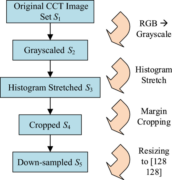
Diagram of preprocessing (color figure online)

Table 3 compares the size and storage per image at every preprocessing step. We can see here after the five-step preprocessing procedure, each image will only cost about 0.52% of its original storage. The byte compression ratio (BCR) was calculated as: $\text{BCR}=\text{byte}\left(s_5\right)÷\text{byte}\left(s_1\right)=65,536÷12,582,912=0.52\%$.

Table 3.

Image size and storage per image at each preprocessing step

Preprocessing step	Image Size (per image)	Byte(s) (per image)
Original $s_1$	$1024\times 1024\times 3=3,145,728$	12,582,912
Grayscaled $s_2$	$1024\times 1024\times 1=1,048,576$	4,194,304
Histogram stretched ${\text{s}}_3$	$1024\times 1024\times 1=1,048,576$	4,194,304
Cropped $s_4$	$724\times 724\times 1=524,176$	2,096,704
Downsampled $s_5$	$128\times 128\times 1=16,384$	65,536

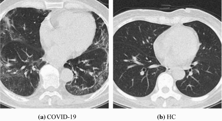
Figure 2 shows two samples of our collected and preprocessed dataset $S_5$, from which we can clearly observe the clinical biomarkers of COVID-19. Cui et al. [19] reported the preliminary CT findings of COVID-19 in their publication. Tuncer et al. [20] used chest CT images, and then developed a local binary pattern and iterative ReliefF algorithm. There are more open publications that show it is feasible to develop effective AI systems based on CCT images.

Fig. 2.

Two samples of our preprocessed dataset ${\mathit{S}}_5$

Basics of DCNN

Deep convolutional neural network (DCNN) is a king of new artificial neural network. Its main feature is to use multiple layers to build a deep neural network. Generally, DCNN is composed of conv layers (CLs), pooling layers (PLs), and fully connected layers (FCLs) [21–25]. Figure 3 presents a simplistic instance consisting of 2 CLs, 2 PLs, and 2 FCLs. On the right part of Fig. 3, The blue rectangle means FCL block, and red rectangle means the softmax function. DCNNs could reach better performances than old-dated AI methods, because they learn the feature from the data during the training procedure. There is no need to consume much time in feature engineering.

Fig. 3.

Pipeline of a toy example of DCNN with 2 CLs, 2PLs, and 2 FCLs

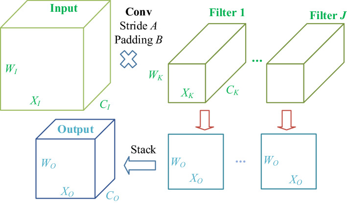
The essential operation in DCNN is convolution. The CL performed 2D convolution along the width and height directions. Note that the weights in CNN are initialized with random, and then learnt from data itself by network training. Figure 4 illustrates the pipeline of input feature maps passing across a CL. Assume there is an input matrix, $J$ kernels ($K_1,K_2,\dots ,K_j,\dots ,K_J$), and an output O, with theirs sizes $\mathbb{S}$ defined as

$$\mathbb{S}\left(x\right)=\left\{\begin{array}{cc}{W}_I\times X_I\times C_I& x=I\\ W_K\times X_K\times C_K& x=K_j\left(j=1,\dots ,J\right)\\ W_O\times X_O\times C_O& x=O\end{array},\right)$$ 8

Fig. 4.

Pipeline of conv layer

where $\left(W,X,C\right)$ represent the size of height, width, and channels of the matrix, respectively. Subscript I, K, and O represent input, kernel, and output, respectively. J denotes total number of filters. Note that

$$C_I=C_K$$ 9a

$$C_O=J$$ 9b

which means the channel of input $C_I$ should equal the channel of kernel $C_K$, and the channel of output $C_O$ should equal the number of filters J.

Assume those filters move with padding of B and stride of A, we can get their relationship by simple math as:

$$W_O=1+\frac{\left(2\times B+W_I-W_K\right)}{A}$$ 10a

$$X_O=1+\frac{\left(2\times B+X_I-X_K\right)}{A},$$ 10b

where $\lfloor .\rfloor$ represents the floor function. Afterward, CL’s outputs are hurled into a nonlinear activation function (NLAF) $\sigma$, that usually selects the rectified linear unit (ReLU) function.

$$\begin{array}{cc}\hfill {\sigma }_{\text{ReLU}}\left(x\right)& =\text{ReLU}\left(x\right)\hfill \\ \hfill & =max\left(0,x\right).\hfill \\ \hfill \end{array}$$ 11

ReLU is preferred to traditional NLAFs such as hyperbolic tangent (HT) and sigmoid (SM) function

$$\begin{array}{cc}\hfill {\sigma }_{\text{HT}}\left(x\right)& =tanh\left(x\right)\hfill \\ \hfill & =\frac{\left(e^x-e^{-x}\right)}{\left(e^x+e^{-x}\right)}\hfill \\ \hfill \end{array}$$ 12

$${\sigma }_{\text{SM}}\left(x\right)={\left(1+e^{-x}\right)}^{-1}.$$ 13

Improvement 1: Use SP to replace MP and AP

The activation maps (AMs) after each block within DCNN are usually too large, i.e., the size of their width, length, and channels are too large to handle, which will cause (i) overfitting of the training and (ii) large computational costs.

Pooling layer (PL) is a form of nonlinear downsampling (NLDS) method to solve above issue. Further, PL can provide invariance-to-translation property to the AMs. For a $2\times 2$ region, suppose the pixels within the region $\overline{\phi }$ are

$$\overline{\phi }=\left[\begin{array}{cc}{\phi }_{1,1}& {\phi }_{1,2}\\ {\phi }_{2,1}& {\phi }_{2,2}\end{array}\right].$$ 14

The average pooling (AP) calculates the mean value in the region $\overline{\phi }$. Assume the output value after NLDS is z, we can have

$$\begin{array}{cc}\hfill z_{\overline{\phi }}^{\mathit{AP}}& =\text{average}\left(\overline{\phi }\right)\hfill \\ \hfill & =\frac{{\phi }_{1,1}+{\phi }_{1,2}+{\phi }_{2,1}+{\phi }_{2,2}}{\left|\overline{\phi }\right|},\hfill \\ \hfill \end{array}$$ 15

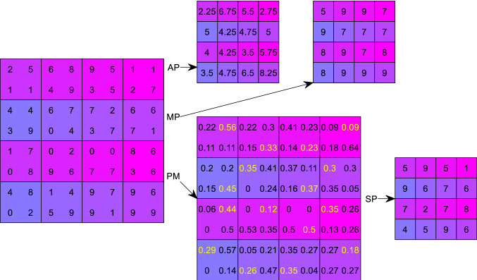
where $\left|\overline{\phi }\right|$ means the number of elements of region $\overline{\phi }$. Here, $\left|\overline{\phi }\right|=4$ if we use a $2\times 2$ NLDS pooling. Using Fig. 5 as an example, and assuming the region $\dot{\phi }$ at 2^nd row 1^st column of the input AM, I is chosen, i.e., $\dot{\phi }=I\left(row=2,col=1\right)$; thus, we have $\begin{array}{c}{z}_{\dot{\phi }}^{\mathit{AP}}=\text{average}\left(\dot{\phi }\right)=\left(4+4+3+9\right)÷4=20÷4=5\end{array}$.

Fig. 5.

Toy examples of different pooling technologies

The max pooling (MP) operates on the region $\overline{\phi }$ and selects the max value. Note that both AP and MP work on every slice separately.

$$\begin{array}{cc}\hfill z_{\overline{\phi }}^{\mathit{MP}}& =max\left(\overline{\phi }\right)\hfill \\ \hfill & ={max}_{i,j=1}^2{\phi }_{i,j}.\hfill \\ \hfill \end{array}$$ 16

In Fig. 5, $\begin{array}{c}{z}_{\dot{\phi }}^{\mathit{MP}}=max\left(\dot{\phi }\right)=max\left(4+4+3+9\right)=9\end{array}$.

In practice, scholars observed that the AP did not work well, because all pixels in the region $\overline{\phi }$ are within the arguments of the NLDS function; hence, it could down-weight (DW) intense activation owing to numerous near-zero pixels. For example, in our region $\dot{\phi }$, the strongest value $9\stackrel{\mathrm{DM}}{\to }5$. On the other hand, MP deciphers above DW problem; however, it simply overfits the training set and causes the lack-of-generalization (LoG) problem.

The stochastic pooling (SP) was introduced to conquer the DW, overfitting, and LoG problems caused by MP and AP. Instead of computing the average or the max, the output of the SP $z^{\text{SP}}$ is calculated via sampling from a multinomial distribution generated from the activations of each region $\overline{\phi }$. Three steps of SP are depicted below:

1. Estimate the probability ${\theta }_{i,j}\in \mathrm{\Theta }$ of each entry $\left\{{\phi }_{i,j},i,j=1,2\right\}$ within the region $\overline{\phi }$.

   $${\theta }_{i,j}=\frac{{\phi }_{i,j}}{\text{sum}\left(\overline{\phi }\right)},i,j=1,2$$ 17a

   $$\sum _{i,j=1}^2{\theta }_{i,j}=1$$ 17b

   in which, (i, j) is the element index of region $\overline{\phi }$. In matrix format, equation (17a) can be rewritten as

   $$\mathrm{\Theta }=\overline{\phi }/\sum \left(\overline{\phi }\right).$$ 18
2. Select a location $\beta$ within $\overline{\phi }$ in accordance with the probability $\left\{{\theta }_{i,j}\right\}$.

   $$\beta \sim \text{Prob}\left({\theta }_{1,1},{\theta }_{1,2},{\theta }_{2,1},{\theta }_{2,2}\right).$$ 19
3. The output is the value at location $\beta$.

   $$z_{\overline{\phi }}^{\text{SP}}={\phi }_{\beta }$$ 20

Use the region $\dot{\phi }$ in Fig. 5 as example, SP first calculates the probability map (PM),

$$\begin{array}{c}\mathrm{\Theta }\left(\dot{\phi }\right)=\left[\begin{array}{cc}4& 4\\ 3& 9\end{array}\right]/\sum \left(\left[\begin{array}{cc}4& 4\\ 3& 9\end{array}\right]\right)\\ =\left[\begin{array}{cc}0.2& 0.2\\ 0.15& 0.45\end{array}\right]\end{array}$$ 21a

$$\beta \left(\dot{\phi }\right)=\left(2,2\right).$$ 21b

Using the probability map, we randomly select the position $\beta =\left(2,2\right)$ associates with probability of ${\theta }_{2,2}\left(\dot{\phi }\right)=0.45$. Thus, the SP output of $\dot{\phi }$ is $z_{\dot{\phi }}^{\mathrm{SP}}={\dot{\phi }}_{\beta }={\dot{\phi }}_{\left(2,2\right)}=9$. In all, SP uses non-maximal activations from the region $\overline{\phi }$, instead of outputting the greatest value.

Improvement 2: batch normalization transform

The motivation of batch normalization transform (BNT) is the so-called internal covariant shift (ICS), which means the effect of randomness of the distribution of inputs to internal DCNN layers during training. The phenomenon of ICS will worsen the DCNN’s performance.

This study introduced BNT to normalize those internal layer’s inputs $A=\left\{a_i\right\}$ over every mini-batch (suppose its size is m), in order to guarantee the batch normalized output $B=\left\{b_i\right\}$ have a uniform distribution. Mathematically, BNT is to learn a function from

$$\underset{A}{\underbrace{\left\{a_i,i=1,2,\dots ,m\right\}}}\mapsto \underset{B}{\underbrace{\{b_i,i=1,2,\dots ,m\}}}.$$ 22

The empirical mean $\mu$ and empirical variance ${\sigma }^2$ over training set $\text{A}$ can be calculated as

$${\mu }_A=\frac{1}{m}\left(\sum _{i=1}^m{a}_i\right)$$ 23

$${\sigma }_A^2=\frac{1}{m}\sum _{i=1}^m{\left(a_i-{\mu }_A\right)}^2.$$ 24

The input $a_i\in A$ was first normalized to

25

where $\mathrm{\Delta }$ in denominator in Eq. (25) is to enhance the numerical stability. The value of $\mathrm{\Delta }$ is a small constant. $\mathrm{\Delta }={10}^{-5}$ in this study. Now has zero-mean and unit-variance characteristics. In order to have a more expressive deep neural network [26], a transformation is usually carried out as

26

where the parameters $\mathfrak{C}$ and $\mathfrak{D}$ are two learnable parameters during training. The transformed output $b_i\in B$ is then passed to the next layer and the normalized remains internal to current layer.

In the inference stage, we do not have mini-batch anymore. So instead of calculating empirical mean and empirical variance, we will calculate population mean $\underset{\_}{\mu }$ and population variance $\underset{\_}{{\sigma }^2}$, and we have the output $\underset{\_}{b_i}$ at inference stage as

$$\underset{\_}{b_i}=\mathfrak{C}\times \left(\frac{a_i-\underset{\_}{\mu }}{sqrt\left(\underset{\_}{{\sigma }^2}+\mathrm{\Delta }\right)}\right)+\mathfrak{D}.$$ 27

We proposed to use convolution block (CB) to be one of the building blocks of our DCNN. The CB consists of one conv layer and one batch normalization layer.

Improvement 3: fully connected block

In traditional DCNN, the fully connected layer (FCL) serves the role of classifier. We plan to replace FCL with fully connected block (FCB), which will include one dropout layer (DOL) and one FCL layer. Srivastava et al. [27] proposed the concept of dropout neurons (DON) and DOL by randomly drop neurons and set to zero their neighboring weights $s$ from the DCNN during training.

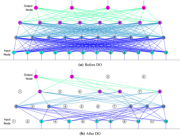
The neuron’s incoming and outgoing connections are freezing, after it is dropped out. Figure 6 illustrates the illustration of neurons in DOL. The selections of dropout are random with a retention probability (${\theta }_{\mathit{rp}}$).

$$\underset{\text{training}}{\tilde{s}}=\left\{\begin{array}{cc}s& \text{with}{\theta }_{\mathit{rp}}\\ 0& \text{otherwise}\end{array}.\right)$$ 28

where ${\theta }_{\mathit{rp}}=0.5$, and $\tilde{s}$ means the weights of dropped out neurons.

Fig. 6.

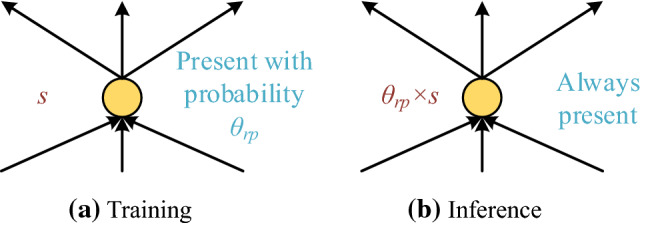
DONs at training and inference stages ($\mathit{s}$ = weights, ${\mathit{\theta }}_{\mathit{r}\mathit{p}}$=retention probability)

During inference, we run the entire DCNN without dropout, but the weights of FCLs of FCBs are downscaled (viz., multiplied) by ${\theta }_{\mathit{rp}}$.

$$\underset{\text{inference}}{\tilde{s}}={\theta }_{\mathit{rp}}\times s.$$ 29

Figure 7 shows a toy DCNN example with four FCL layers. Suppose we have $N\left(k\right)$ neurons at k-th layer, and assume $N\left(1\right)=12$, $N\left(2\right)=10$, $N\left(3\right)=8$, $N\left(4\right)=4$. Thus, we have in total ${\sum }_{k=1}^{4}N\left(k\right)=34$ nodes. Suppose we do not consider incoming and outgoing weights, and do not consider the number of biases, the size of learnable weights $S^b\left(i,j\right)$ as number of weights between layer $i$ and layer $j$ before dropout, roughly calculating, can be written as $S^b\left(1,2\right)=12\times 10=120$, $S^b\left(2,3\right)=10\times 8=80$, $S^b\left(3,4\right)=8\times 4=32$. In total, we have the total number of learnable weights before dropout as $S^b={\sum }_{k=1}^3{S}^b\left(k,k+1\right)=232$. Using ${\theta }_{\mathit{rp}}=0.5$, the size of learnable weights after dropout between layer $i$ and layer $j$ is symbolized as $S^a(i,j)$, and we can calculate the total number of learnable weights as $S^a={\sum }_{k=1}^3{S}^a\left(k,k+1\right)=S^a\left(1,2\right)+S^a\left(2,3\right)+S^a\left(3,4\right)=30+20+8=58$.

Fig. 7.

A toy example of a DCNN with four FCLs

The compression ratio of learnable weights (CRLW), roughly, can be calculated by $58/232=0.25$, which is the squared value of retention probability ${\theta }_{\mathit{rp}}$.

$$\text{CRLW}=\frac{S^a}{S^b}={\theta }_{\mathit{rp}}^2,$$ 30

where $S^a$ and $S^b$ means the number of learnable weights after and before dropout, respectively.

Proposed DCNN and its Implementation

We create a new five-layer DCNN with stochastic pooling for COVID-19 detection (5L-DCNN-SP-C) with three CBs and two FCBs. The structure of proposed 5L-DCNN-SP-C is shown in Fig. 8, where SP is added after each activation map. The reason why set three CBs and two FCBs are by manual trial-and-error method. In the experiment, we will compare this setting (3 CBs + 2 FCBs) against other setting.

Fig. 8.

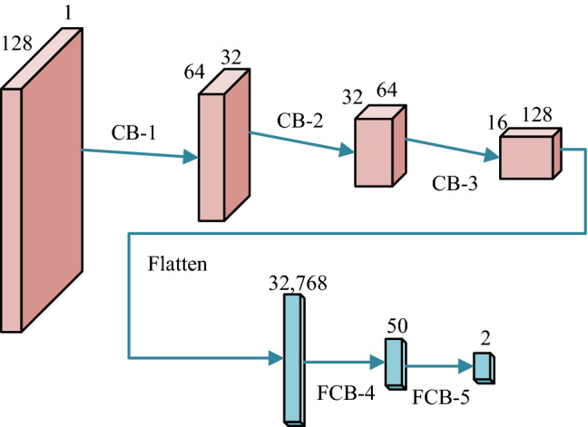
Structure of proposed 5L-DCNN-SP-C

The hyperparameters of each layer/block of proposed 5L-DCNN-SP-C are listed in Table 4, where $\left(\alpha \beta \times \beta /\gamma \right)$ means $\alpha$ filters with size of $\beta \times \beta$, followed by pooling layer with pooling size of $\gamma$. Meanwhile, W and B represent the size of weight matrix and bias vector, respectively. The last column in Table 4 shows the activation map (AM).

Table 4.

Details of each layer in proposed 5L-DCNN-SP-C

Layer/Block	Hyperparameter	AM
Input	n/a	128 × 128 × 1
CB-1-SP	32 3 × 3 /2	64 × 64 × 32
CB-2-SP	64 3 × 3 /2	32 × 32 ×  64
CB-3-SP	128 3 × 3 /2	16 × 16 × 128
Flatten		1 ×  32,768
FCB-4	W(50 × 32,768); B(50 × 1); ${\theta }_{\mathit{rp}}=0.5$	1 × 50
FCB-5	W(2 × 50); B(2 × 1); ${\theta }_{\mathit{rp}}=0.5$	1 × 2

n/a   not available, AM   activation map

Ten runs of tenfold cross-validation were employed. Suppose confusion matrix $\mathbb{C}$ is defined as

$$\mathbb{C}\left(k,r\right)=\left[\begin{array}{cc}{c}_{11}& c_{12}\\ c_{21}& c_{22}\end{array}\right],$$ 31

where $\left(c_{11},c_{12},c_{21},c_{22}\right)$ represent TP, FN, FP, and TN, respectively. k is the index of trial (in each trial, onefold was used as test, and all the other folds were used as training), and r is the index of run.

Note that $\mathbb{C}$ will be calculated based on each test fold, and summarized across all 10 trials. Then, we get the

$$\mathbb{C}\left(r\right)=\sum _{k=1}^{10}\mathbb{C}\left(k,r\right).$$ 32

Now we can calculate six indicators $\overrightarrow{\eta }\left(r\right)$ based on the confusion matrix over r-th run $\mathbb{C}\left(r\right)$.

$$\mathbb{C}\left(r\right)\mapsto \underset{\overrightarrow{\eta }\left(r\right)}{\underbrace{\left[{\eta }_1\left(r\right),{\eta }_2\left(r\right),\dots ,{\eta }_6\left(r\right)\right]}},$$ 33

where ${\eta }_1$ is sensitivity, ${\eta }_2$ is specificity, ${\eta }_3$ is precision, and ${\eta }_4$ is accuracy. Ignoring variable r, we have:

$${\eta }_1=\frac{c_{11}}{c_{11}+c_{12}}$$ 34a

$${\eta }_2=\frac{c_{22}}{c_{22}+c_{21}}$$ 34b

$${\eta }_3=\frac{c_{11}}{c_{11}+c_{21}}$$ 34c

$${\eta }_4=\frac{c_{11}+c_{22}}{c_{11}+c_{12}+c_{21}+c_{22}}$$ 34d

${\eta }_5$ is F1 score.

$${\eta }_5=2\times \frac{{\eta }_3\times {\eta }_1}{{\eta }_3+{\eta }_1}=\frac{2\times c_{11}}{2\times c_{11}+c_{12}+c_{21}}$$ 35

and ${\eta }_6$ is Matthews correlation coefficient (MCC)

$${\eta }_6=\frac{c_{11}\times c_{22}-c_{21}\times c_{12}}{\sqrt{\left(c_{11}+c_{21}\right)\times \left(c_{11}+c_{12}\right)\times \left(c_{22}+c_{21}\right)\times \left(c_{22}+c_{12}\right)}}.$$ 36

The mean and standard deviation (SD) of all six measures $\overrightarrow{\eta }$ will be calculated over all ten runs.

$$\text{mean}\left({\eta }_m\right)=\frac{1}{10}\times \sum _{r=1}^{10}{\eta }_m\left(r\right)$$ 37a

$$\text{SD}\left({\eta }_m\right)=\sqrt{\frac{1}{9}\times \sum _{r=1}^{10}{\left|{\eta }_m\left(r\right)-\text{mean}\left({\eta }_m\right)\right|}^2},$$ 37b

where $1\le m\le 6$ represents the index of measures.

Experiments, results, and discussion

Pooling method comparison

The results of 10 runs $\overrightarrow{\eta }$ of SP were compared against AP and MP. We compared three pooling methods on test set. The results of all three pooling methods are listed in Table 5. For AP, it obtains ${\eta }_1=91.22\pm 1.35$, ${\eta }_2=90.47\pm 1.27$, ${\eta }_3=90.55\pm 1.19$, ${\eta }_4=90.84\pm 1.05$, ${\eta }_5=90.88\pm 1.06$, and ${\eta }_6=81.70\pm 2.10$. The results of AP are the worst of all three pooling methods. MP obtains better results than AP. The six measures of MP are ${\eta }_1=92.38\pm 1.04$, ${\eta }_2=92.75\pm 0.92$, ${\eta }_3=92.73\pm 0.89$., ${\eta }_4=92.56\pm 0.81$, ${\eta }_5=92.55\pm 0.82$, and ${\eta }_6=85.13\pm 1.61$. Finally, SP obtains the greatest performances on all six measures. The six measures of SP are as follows: ${\eta }_1=93.28\pm 1.50$, ${\eta }_2=94.00\pm 1.56$, ${\eta }_3=93.96\pm 1.54$, ${\eta }_4=93.64\pm 1.42$, ${\eta }_5=93.62\pm 1.42$, and ${\eta }_6=87.29\pm 2.83$. For the ease of clear view, Fig. 9 presents the error bar plot of comparison of all three pooling methods.

Table 5.

Ten runs of AP, MP, and SP

AP	${\eta }_1$	${\eta }_2$	${\eta }_3$	${\eta }_4$	${\eta }_5$	${\eta }_6$
1	93.13	90.00	90.30	91.56	91.69	83.17
2	90.94	90.00	90.09	90.47	90.51	80.94
3	92.50	90.94	91.08	91.72	91.78	83.45
4	90.94	92.19	92.09	91.56	91.51	83.13
5	91.56	90.63	90.71	91.09	91.14	82.19
6	91.88	92.50	92.45	92.19	92.16	84.38
7	90.94	90.63	90.65	90.78	90.80	81.56
8	92.19	89.38	89.67	90.78	90.91	81.59
9	88.75	90.31	90.16	89.53	89.45	79.07
10	89.38	88.13	88.27	88.75	88.82	77.51
Mean ± SD	91.22 ± 1.35	90.47 ± 1.27	90.55 ± 1.19	90.84 ± 1.05	90.88 ± 1.06	81.70 ± 2.10

MP	${\eta }_1$	${\eta }_2$	${\eta }_3$	${\eta }_4$	${\eta }_5$	${\eta }_6$
1	90.63	92.50	92.36	91.56	91.48	83.14
2	92.19	92.19	92.19	92.19	92.19	84.38
3	93.44	93.13	93.15	93.28	93.29	86.56
4	93.75	94.38	94.34	94.06	94.04	88.13
5	93.44	93.13	93.15	93.28	93.29	86.56
6	92.81	92.19	92.24	92.50	92.52	85.00
7	91.88	91.56	91.59	91.72	91.73	83.44
8	91.56	91.88	91.85	91.72	91.71	83.44
9	91.25	94.06	93.89	92.66	92.55	85.35
10	92.81	92.50	92.52	92.66	92.67	85.31
Mean ± SD	92.38 ± 1.04	92.75 ± 0.92	92.73 ± 0.89	92.56 ± 0.81	92.55 ± 0.82	85.13 ± 1.61

SP	${\eta }_1$	${\eta }_2$	${\eta }_3$	${\eta }_4$	${\eta }_5$	${\eta }_6$
1	91.25	91.56	91.54	91.41	91.39	82.81
2	95.31	94.69	94.72	95.00	95.02	90.00
3	93.75	95.94	95.85	94.84	94.79	89.71
4	91.25	94.06	93.89	92.66	92.55	85.35
5	95.00	96.25	96.20	95.63	95.60	91.26
6	92.50	92.81	92.79	92.66	92.64	85.31
7	92.19	91.88	91.90	92.03	92.04	84.06
8	95.00	94.38	94.41	94.69	94.70	89.38
9	93.13	93.75	93.71	93.44	93.42	86.88
10	93.44	94.69	94.62	94.06	94.03	88.13
Mean ± SD	93.28 ± 1.50	94.00 ± 1.56	93.96 ± 1.54	93.64 ± 1.42	93.62 ± 1.42	87.29 ± 2.83

Fig. 9.

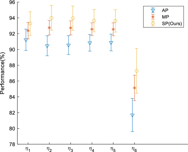
Error bar of different pooling methods

Structure comparison

We set the number of CBs as ${\mathrm{\gamma }}_{\text{CB}}$ and the number of FCB as ${\mathrm{\gamma }}_{\text{FCB}}$. We set ${\mathrm{\gamma }}_{\text{CB}}=3$ and ${\mathrm{\gamma }}_{\text{FCB}}=2$ by trial-and-error method. Suppose we all use SP, and we create five different structure configurations (SC) setting as in Table 6. The results of cognate performances on test set $\overrightarrow{\eta }$ are shown in Table 7, where we can observe the SC-V performs the best results, which corresponds to our optimal SC setting: ${\mathrm{\gamma }}_{\text{CB}}=3$ and ${\mathrm{\gamma }}_{\text{FCB}}=2$

Table 6.

SC setting

SC	${\mathrm{\gamma }}_{\text{CB}}$	${\mathrm{\gamma }}_{\text{FCB}}$
I	2	1
II	2	2
III	2	3
IV	3	1
V (Ours)	3	2
VI	3	3

SC  structure configuration, ${\mathrm{\gamma }}_{\text{CB}}$   number of CBs, ${\mathrm{\gamma }}_{\text{FCB}}$  number of FCBs

Table 7.

Performances of all six SCs (bold means the best)

SC	${\eta }_1$	${\eta }_2$	${\eta }_3$	${\eta }_4$	${\eta }_5$	${\eta }_6$
I	92.28 ± 0.69	91.00 ± 1.53	91.13 ± 1.39	91.64 ± 0.86	91.70 ± 0.82	83.30 ± 1.72
II	93.13 ± 1.32	92.59 ± 1.36	92.65 ± 1.26	92.86 ± 1.00	92.88 ± 1.00	85.73 ± 1.99
III	93.28 ± 0.61	92.97 ± 1.33	93.01 ± 1.23	93.13 ± 0.71	93.14 ± 0.68	86.26 ± 1.43
IV	92.69 ± 1.11	92.53 ± 1.88	92.57 ± 1.71	92.61 ± 1.08	92.62 ± 1.04	85.24 ± 2.14
V (Ours)	93.28 ± 1.50	94.00 ± 1.56	93.96 ± 1.54	93.64 ± 1.42	93.62 ± 1.42	87.29 ± 2.83
VI	93.44  ± 1.52	93.03  ± 1.09	93.07 ± 0.98	93.23  ± 0.82	93.24 ± 0.85	86.49 ± 1.65

Comparison to State-of-the-art approaches

We compare our method “5L-DCNN-SP-C” with other COVID-19 classification approaches: RBFNN [6], K-ELM [7], ELM-BA [8], 6L-CNN-F [9], GoogLeNet [10], ResNet-18 [11]. The results $\overrightarrow{\eta }$ on ten runs over test set are presented in Table 8. It is easily observed that our proposed 5L-DCNN-SP-C smashes all the other six comparison baseline methods in all indicators. Particularly, 6L-CNN-F [9] also used convolutional neural network method, and they used more layers (6 layers) than layers used in our model (5 layers).

Table 8.

Comparison with SOTA approaches (Unit: %)

Approach	${\eta }_1$	${\eta }_2$	${\eta }_3$	${\eta }_4$	${\eta }_5$	${\eta }_6$
RBFNN [6]	67.08	74.48	72.52	70.78	69.64	41.74
K-ELM [7]	57.29	61.46	59.83	59.38	58.46	18.81
ELM-BA [8]	57.08 ± 3.86	72.40 ± 3.03	67.48 ± 1.65	64.74 ± 1.26	61.75 ± 2.24	29.90 ± 2.45
6L-CNN-F [9]	81.04 ± 2.90	79.27 ± 2.21	79.70 ± 1.27	80.16 ± 0.85	80.31 ± 1.13	60.42 ± 1.73
GoogLeNet [10]	76.88 ± 3.92	83.96 ± 2.29	82.84 ± 1.58	80.42 ± 1.40	79.65 ± 1.92	61.10 ± 2.62
ResNet-18 [11]	78.96 ± 2.90	89.48 ± 1.64	88.30 ± 1.50	84.22 ± 1.23	83.31 ± 1.53	68.89 ± 2.33
5L-DCNN-SP-C (Ours)	93.28 ± 1.50	94.00 ± 1.56	93.96 ± 1.54	93.64 ± 1.42	93.62 ± 1.42	87.29 ± 2.83

The reason why our five-layer model is better than that six-layer model [9] is threefold: (i) We choose SP to improve the performance of our deep learning model; (ii) We fine-tune the hyperparameters (such as ${\mathrm{\gamma }}_{\text{CB}}$, ${\mathrm{\gamma }}_{\text{FCB}}$, number of filters at each CB, number of neurons at each FCB); (iii) Our model was particularly designed for detecting COVID-19, while the 6L-CNN-F [9] was designed for fingerspelling recognition. In the future, we shall try to use clustering techniques [28, 29] to help improve the performance. Figure 10 shows the comparison bar plot of all seven methods.

Fig. 10.

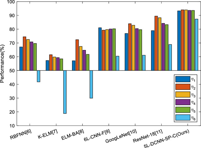
Comparison to state-of-the-art approaches

Conclusion

This study proposed a novel 5L-DCNN-SP-C framework, that combines deep convolutional neural network and stochastic pooling for COVID-19 diagnosis. We added batch normalization transform and dropout layers, and proposed two new blocks (convolution block and fully connected block). In our test, we proved three CBs and two FCBs structure can give the best performance.

There are several shortcomings of our method: (i) The dataset is somewhat small. We shall seek to collect more datasets. (ii) Some new network technologies would be tried in our future studies, such as the recent transfer learning pretrained models.

Biographies

Prof. Yu-Dong Zhang

received his Ph.D. degree in Signal and Information Processing from Southeast University in 2010. He worked as a postdoc from 2010 to 2012 with Columbia University, USA, and as an assistant research scientist from 2012 to 2013 with Research Foundation of Mental Hygiene (RFMH), USA. Now he serves as a Professor with Department of Informatics, University of Leicester, UK. His research interests include deep learning and medical image analysis.

Dr. Suresh Chandra Satapathy

is Ph.D. in Computer Science Engineering, currently working as Professor of School of Computer Engg and Dean—Research at KIIT (Deemed to be University), Bhubaneshwar, Odisha, India. He has developed two new optimization algorithms known as Social Group Optimization (SGO) published in Springer Journal and SELO (Social Evolution and Learning Algorithm) published in Elsevier. He has more than 150 publications in reputed journals and conf proceedings.

Dr. Shuaiqi Liu

received his Ph.D. degree in Institute of Information Science from Beijing Jiaotong University in 2014 and got B.S. degree in the Department of Information and Computer Science from Shandong University of Science and Technology in 2009. At present, he is an associate professor in College of Electronic and Information Engineering, Hebei University. And he is a visiting scholar at Ottawa University from August 2016 to January 2017. His research interests include image processing and signal processing.

Professor Guang-Run Li

obtained a bachelor's degree from Nanjing Medical University in 2005. He is currently the director of the Department of Imaging of Jinhu People's Hospital. He has presided over several municipal scientific research projects and published more than 20 papers. His main research interests are imaging technology and diagnosis, artificial intelligence, including the application of radiology and deep learning in imaging.

References

- 1.Hadi AG, Kadhom M, Hairunisa N, Yousif E, Mohammed SA. A review on COVID-19: origin, spread, symptoms, treatment, and prevention. Biointerface Res. Appl. Chem. 2020;10:7234–7242. doi: 10.33263/BRIAC106.72347242. [DOI] [Google Scholar]
- 2.Tsuchida T, Fujitani S, Yamasaki Y, Kunishima H, Matsuda T. Development of a protective device for RT-PCR testing SARS-CoV-2 in COVID-19 patients. Infect. Control Hosp. Epidemiol. 2020;41:975–976. doi: 10.1017/ice.2020.121. [DOI] [PMC free article] [PubMed] [Google Scholar]
- 3.Penarrubia L, Ruiz M, Porco R, Rao SN, Juanola-Falgarona M, Manissero D, et al. Multiple assays in a real-time RT-PCR SARS-CoV-2 panel can mitigate the risk of loss of sensitivity by new genomic variants during the COVID-19 outbreak. Int. J. Infect. Dis. 2020;97:225–229. doi: 10.1016/j.ijid.2020.06.027. [DOI] [PMC free article] [PubMed] [Google Scholar]
- 4.Ai, T., Yang, Z., Hou, H., Zhan, C., Chen, C., Lv, W. et al.: Correlation of chest CT and RT-PCR testing in coronavirus disease 2019 (COVID-19) in China: a report of 1014 cases. Radiology, Article ID: 200642, (2020) [DOI] [PMC free article] [PubMed]
- 5.Li Y, Xia L. Coronavirus disease 2019 (COVID-19): role of chest CT in diagnosis and management. AJR Am. J. Roentgenol. 2020;214:1280–1286. doi: 10.2214/AJR.20.22954. [DOI] [PubMed] [Google Scholar]
- 6.Lu Z. A pathological brain detection system based on radial basis function neural network. J. Med. Imaging Health Inform. 2016;6:1218–1222. doi: 10.1166/jmihi.2016.1901. [DOI] [Google Scholar]
- 7.Yang J. A pathological brain detection system based on kernel based ELM. Multimed. Tools Appl. 2018;77:3715–3728. doi: 10.1007/s11042-016-3559-z. [DOI] [Google Scholar]
- 8.Lu S. A pathological brain detection system based on extreme learning machine optimized by bat algorithm. CNS Neurol. Disord. Drug. Targets. 2017;16:23–29. doi: 10.2174/1871527315666161019153259. [DOI] [PubMed] [Google Scholar]
- 9.Jiang X. Chinese sign language fingerspelling recognition via six-layer convolutional neural network with leaky rectified linear units for therapy and rehabilitation. J. Med. Imaging Health Inform. 2019;9:2031–2038. doi: 10.1166/jmihi.2019.2804. [DOI] [Google Scholar]
- 10.Szegedy, C., Liu, W., Jia, Y., Sermanet, P., Reed, S., Anguelov, D. et al.: Going deeper with convolutions. In: Proceedings of the IEEE conference on computer vision and pattern recognition, 2015, pp. 1–9.
- 11.Yu X, Wang S-H. Abnormality diagnosis in mammograms by transfer learning based on ResNet18. Fundam. Inform. 2019;168:219–230. doi: 10.3233/FI-2019-1829. [DOI] [Google Scholar]
- 12.Albahri, A.S., Hamid, R.A., Alwan, J.K., Al-qays, Z.T., Zaidan, A.A., Zaidan, B.B. et al.: Role of biological data mining and machine learning techniques in detecting and diagnosing the novel coronavirus (COVID-19): a systematic review. J. Med. Syst. 44, 11, Article ID: 122, (2020). [DOI] [PMC free article] [PubMed]
- 13.De Felice F, Polimeni A. Coronavirus Disease (COVID-19): A Machine Learning Bibliometric Analysis. In Vivo. 2020;34:1613–1617. doi: 10.21873/invivo.11951. [DOI] [PMC free article] [PubMed] [Google Scholar]
- 14.Liu AJ. Tea category identification using computer vision and generalized eigenvalue proximal SVM. Fundam. Inform. 2017;151:325–339. doi: 10.3233/FI-2017-1495. [DOI] [Google Scholar]
- 15.Zhan TM, Chen Y. Multiple sclerosis detection based on biorthogonal wavelet transform, RBF kernel principal component analysis, and logistic regression. IEEE Access. 2016;4:7567–7576. doi: 10.1109/ACCESS.2016.2620996. [DOI] [Google Scholar]
- 16.Du S. Multi-objective path finding in stochastic networks using a biogeography-based optimization method. Simulation. 2016;92:637–647. doi: 10.1177/0037549715623847. [DOI] [Google Scholar]
- 17.Atangana A. Application of stationary wavelet entropy in pathological brain detection. Multimed. Tools Appl. 2018;77:3701–3714. doi: 10.1007/s11042-016-3401-7. [DOI] [Google Scholar]
- 18.Pan H, Zhang C, Tian Y. RGB-D image-based detection of stairs, pedestrian crosswalks and traffic signs. J. Vis. Commun. Image Represent. 2014;25:263–272. doi: 10.1016/j.jvcir.2013.11.005. [DOI] [Google Scholar]
- 19.Cui N, Zou XG, Xu L. Preliminary CT findings of coronavirus disease 2019 (COVID-19) Clin. Imaging. 2020;65:124–132. doi: 10.1016/j.clinimag.2020.04.042. [DOI] [PMC free article] [PubMed] [Google Scholar]
- 20.Tuncer, T., Dogan, S., Ozyurt, F.: An automated residual exemplar local binary pattern and iterative ReliefF based COVID-19 detection method using chest X-ray image. Chemom. Intell. Lab. Syst. 203, 11, Article ID: 104054, (2020) [DOI] [PMC free article] [PubMed]
- 21.Hong J. Classification of cerebral microbleeds based on fully-optimized convolutional neural network. Multimed. Tools Appl. 2020;79:15151–15169. doi: 10.1007/s11042-018-6862-z. [DOI] [Google Scholar]
- 22.Hong J. Sensorineural hearing loss identification via nine-layer convolutional neural network with batch normalization and dropout. Multimed. Tools Appl. 2020;79:15135–15150. doi: 10.1007/s11042-018-6862-z. [DOI] [Google Scholar]
- 23.Wang S, Chen Y. Fruit category classification via an eight-layer convolutional neural network with parametric rectified linear unit and dropout technique. Multimed. Tools Appl. 2020;79:15117–15133. doi: 10.1007/s11042-018-6661-6. [DOI] [Google Scholar]
- 24.Sui, Y.X.: Classification of Alzheimer's disease based on eight-layer convolutional neural network with leaky rectified linear unit and max pooling. J. Med. Syst. vol. 42, Article ID: 85, (2018) [DOI] [PubMed]
- 25.Jiang YY. Cerebral micro-bleed detection based on the convolution neural network with rank based average pooling. IEEE Access. 2017;5:16576–16583. doi: 10.1109/ACCESS.2017.2736558. [DOI] [Google Scholar]
- 26.Garbin C, Zhu XQ, Marques O. Dropout versus batch normalization: an empirical study of their impact to deep learning. Multimed. Tools Appl. 2020;79:12777–12815. doi: 10.1007/s11042-019-08453-9. [DOI] [Google Scholar]
- 27.Srivastava N, Hinton G, Krizhevsky A, Sutskever I, Salakhutdinov R. Dropout: a simple way to prevent neural networks from overfitting. J. Mach. Learn. Res. 2014;15:1929–1958. [Google Scholar]
- 28.Chen Y, Zhou L, Pei S, Yu Z, Chen Y, Liu X, et al. KNN-BLOCK DBSCAN: fast clustering for large-scale data. IEEE Trans. Syst. Man Cybern. Syst. 2019 doi: 10.1109/TSMC.2019.2956527. [DOI] [Google Scholar]
- 29.Chen, Y.W., Hu, X.L., Fan, W.T., Shen, L.L., Zhang, Z., Liu, X. et al.: Fast density peak clustering for large scale data based on kNN. Knowl. Based Syst. 187, 7. Article ID: 104824