Identifying genetic variants underlying phenotypic variation in plants without complete genomes

Abstract

Structural variants and presence/absence polymorphisms are common in plant genomes, yet they are routinely overlooked in genome-wide association studies (GWAS). Here, we expand the type of genetic variants detected in GWAS to include major deletions, insertions, and rearrangements. We first use raw sequencing data directly to derive short sequences, k-mers, that mark a broad range of polymorphisms independently of a reference genome. We then link k-mers associated with phenotypes to specific genomic regions. Using this approach, we re-analyzed 2,000 traits in Arabidopsis thaliana, tomato, and maize populations. Associations identified with k-mers recapitulate those found with single-nucleotide polymorphisms (SNPs), but with stronger statistical support. Importantly, we discovered new associations with structural variants and with regions missing from reference genomes. Our results demonstrate the power of performing GWAS before linking sequence reads to specific genomic regions, which allows detection of a wider range of genetic variants responsible for phenotypic variation.

Genome-wide association studies (GWAS) support the systematic identification of candidate genomic loci responsible for phenotypic variation. A difficulty with plants is that their genomes are characterized by many structural variants (SV), which can often cause phenotypic variation¹. Although this is not usually done, short sequencing reads can provide, in principle, information for many more variants in their source genomes than SNPs and short insertions/deletions (indels)². Variants are typically discovered with short reads by mapping them to a reference genome, but one can also directly compare common subsequences among samples^3,4. Such a direct approach is intuitively most powerful when there is no or only a poor reference genome assembly. Because short reads result from random shearing of genomic DNA, and because they contain sequencing errors, comparing short reads between two samples directly is, however, not very effective. Instead, genetic variants in a population can be discovered by focusing on sequences of constant length k that are shorter than the original reads, termed k-mers. After k-mers have been extracted from all reads, k-mer sets from different samples can be compared against each other. Importantly, k-mers present in some samples, but missing from others, can identify a broad range of genetic variants. For example, two genomes differing in a SNP (Fig. 1A, Extended Data Fig. 1,2) will have k k-mers unique to each genome; this is true even if the SNP is found in a repeated region or a region not found in the reference genome. SVs, such as large deletions, inversions, translocations, etc. will also result in k-mer differences. Therefore, instead of defining genetic variants in a population relative to a reference genome, a k-mer presence/absence pattern in raw sequencing data can be directly associated with phenotypes to enlarge the tagged genetic variants in GWAS⁵.

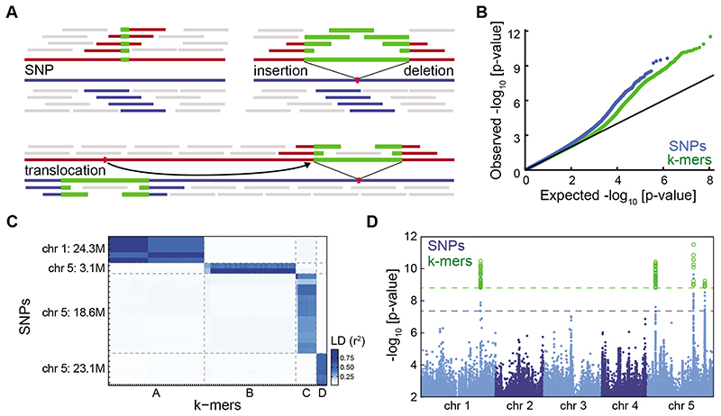
Figure 1. Flowering time associations in A. thaliana .

(A) k-mers and different genetic variants. Blue and red lines represent two individual genomes. Colored short bars mark k-mers unique to each genome; grey bars k-mers shared between genomes.

(B) p-value quantile-quantile plot of SNP and k-mer associations with flowering time in 10°C. Deviation from y=x indicates stronger than chance associations.

(C) LD between SNPs and k-mers passing p-value thresholds. Both methods identified four highly linked families of variants. For SNP-to-SNP and k-mer-to-k-mer LD, see Extended Data Fig. 5A,B.

(D) p-values of all SNPs (blue) and of the subset of k-mers passing the p-value threshold (green) as a function of their genomic position. Dashed lines mark the thresholds for SNPs (blue) and k-mers (green). Extended Data Fig. 5C,D shows separate figures for k-mers and SNPs.

Reference-free GWAS based on k-mers has been used with bacteria, which have many dispensable genes^5–7. It has also been applied to human genomes, which are much larger and have many more unique k-mers^3,8, but this was restricted to case-control situations, and due to high computational load, population structure was not corrected for all k-mers. While k-mer based approaches are likely to be especially appropriate for plants, their large genomes, highly structured populations, and excessive genetic variation^9–11 make the use of existing k-mer methods difficult. An attempt with k-mers in plants was limited to a small subset of the genome, and also accounted for population structure only for a small subset of k-mers¹².

Here, we present an efficient method for k-mer-based GWAS and compare it directly to the conventional SNP-based approach on more than 2,000 phenotypes from three species with different genome and population characteristics - A. thaliana, maize and tomato. In brief, we have inverted the conventional approach of building a genome, using it to find population variants, and finally associating variants with phenotypes. In contrast, we begin by associating sequencing reads with phenotypes, and only then infer the genomic context of associated sequences. We posit that this change of order is especially effective in plants, for which defining the full population-level genetic variation based on reference genomes remains highly challenging.

Results

Comparison of SNP and k-mer GWA on A. thaliana phenotypes

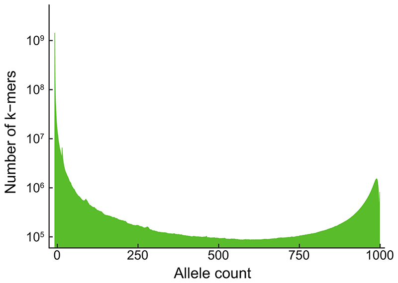
As an initial proof of concept, we looked at a model trait, flowering time in A. thaliana. We used an existing dataset¹³ to define the presence/absence patterns of 31 bp k-mers in over 1,000 inbred accessions. Out of a total 2.26 billion unique k-mers, 439 million appeared in at least five accessions (Extended Data Fig. 3A, 4). Using k-mer presence/absence as two allelic contrasts, we performed GWA with a linear mixed model (LMM) to account for population structure (Extended Data Fig. 3B)¹⁴, and compared it to GWA with SNPs and short indels (Fig. 1B).

To define a set of k-mers most likely to be associated with flowering time, we had to set a p-value threshold. Unfortunately, a single genetic variant is typically tagged by several k-mers, and the Bonferroni threshold would not accurately reflect the effective number of independent tests. To account for non-independence, we defined a threshold based on permutations of the phenotype¹⁵. This is computationally challenging, as the full GWA analysis has to be run many times. We therefore implemented a LMM-based GWA specifically optimized for the k-mers application (Extended Data Fig. 3C)^16,17.

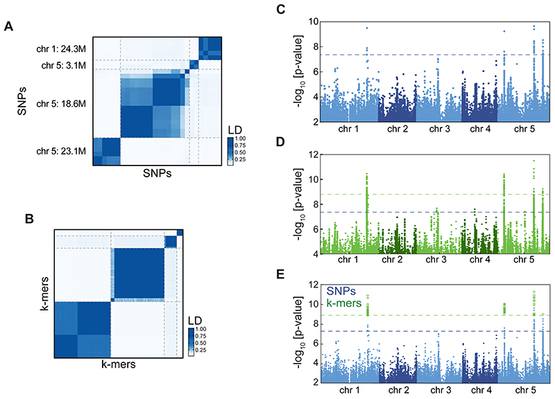
We calculated the p-value thresholds for SNPs and k-mers, with a 5% chance of one false-positive. The threshold for k-mers was higher than SNPs (35-fold), but lower than the increase in test number (140-fold), due to the higher dependency between k-mers (Fig. 1A). Twenty-eight SNPs and 105 k-mers passed their corresponding thresholds. Using LD, we linked SNPs to k-mers directly without locating the k-mers in the genome. Four families of linked genetic variants were identified with both methods (Fig. 1C). As expected, the k-mers tagged the same genomic loci as the corresponding SNPs (Fig. 1D, for 25 bp k-mers, Extended Data Fig. 5E). Therefore, k-mers identified the same genotype-flowering time associations as SNPs.

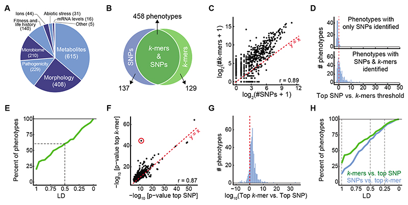
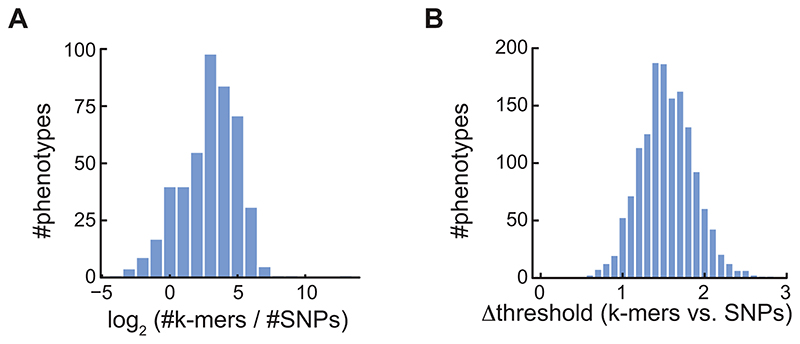
To increase the chances of discovering new associations, we evaluated 1,582 phenotypes from 104 A. thaliana studies (Supplementary Table 1, Fig. 2A). There was substantial overlap in significant SNP and k-mer associations (Fig. 2B), with k-mer and SNP hits numbers for each phenotype being highly correlated (Fig. 2C, Extended Data Fig. 6A). For 137 phenotypes, only a significant SNP could be identified, likely due to the more stringent thresholds for k-mers, as the most significant SNPs rarely passed the k-mer threshold in these cases (Fig. 2D). Moreover, often, a k-mer passing the SNPs threshold was in high LD with the top SNP (Fig. 2E). Although the k-mer thresholds were more stringent than the SNPs thresholds (Extended Data Fig. 6B), for 129 phenotypes only k-mers but no SNPs associations were identified. The p-values of top SNPs and k-mers were highly correlated (Fig. 2F), with top k-mers having a lower p-value in almost 9 out of 10 cases (Fig. 2G). In addition, we found that associated k-mers were on average closer to top SNPs than the other way around: 29% of top SNPs were in complete LD with associated k-mers vs. 13% the other way around, and 73% vs. 67% in LD≥0.5 (Fig. 2H), consistent with k-mers often containing the top SNP, but SNPs in many cases only being linked to the causal variant identified by k-mers.

Figure 2. SNP- and k-mer-based GWAS on 1,582 A. thaliana phenotypes.

(A) Categories of collected phenotypes.

(B) Overlap between phenotypes with SNP and k-mer hits.

(C) Correlation of numbers of significant k-mers vs. SNPs.

(D) Ratios (in log₁₀) of top SNP p-value vs. the k-mer threshold for 137 phenotypes with only significant SNPs (top), and for 458 phenotypes with both significant SNPs and k-mers (bottom).

(E) Fraction of phenotypes, from 137 phenotypes that had only significant SNP hits, for which a k-mer passing the SNP threshold could be found within different LD cutoffs. For a minimum of LD=0.5 (dashed lines), 61% of phenotypes had a linked k-mer that passed the SNP threshold.

(F) Correlation of p-values of top k-mers and SNPs (r=0.87). Red circle marks the strongest outlier (see Fig. 3A, B for details on this phenotype).

(G) Ratio between top p-values (expressed as -log₁₀) in the two methods, for the 458 phenotypes with both k-mer and SNP hits.

(H) Fraction of all phenotypes for which a significant SNP could be found within different LD cutoffs of top k-mer (blue) and vice versa (green). Dashed lines mark LD=1, 0.5, and 0.25, with fractions of phenotypes being 29%, 73%, and 90% for the green curve, and 13%, 67%, and 88% for the blue curve, respectively.

Case studies of k-mer superiority

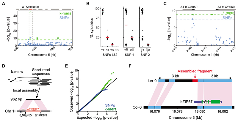
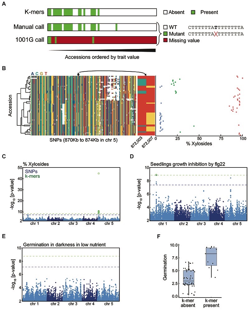
In addition to simply improving the strength of associations (Extended Data Fig. 7A), we sought to identify cases where k-mers provided a conceptual improvement. We first looked at the fraction of dihydroxybenzoic acid (DHBA) xylosides among total DHBA glycosides¹⁸ (red circle, Fig. 2F). In this case, all significant k-mers mapped uniquely near AT5G03490, encoding a UDP glycosyltransferase, already identified in the original study (Fig. 3A, Extended Data Fig. 7C). The stronger k-mer associations could be traced back to two non-synonymous SNPs, 4 bp apart, in the gene’s coding region. Due to their proximity, one k-mer holds the state of both SNPs, and their combined information is more predictive of the phenotype than either SNP alone (Fig. 3B).

Figure 3. Specific cases of k-mer superiority.

(A) Associations with xyloside fraction in indicated region. Boxes on top indicate genes, with AT5G03490 in red.

(B) Xyloside fraction grouped by states at two adjacent SNPs (872,003 and 872,007 bp). Left shows simultaneous grouping based on both SNPs, possible with k-mers. Middle and right, groupings based on only one of the two SNPs. Haplotypes in this region will not capture this association (Extended Data Fig. 7B).

(C) Associations with seedling growth inhibition in the presence of flg22. Absence of SNPs in the central 1 kb region is likely due to the presence of a TE to which short reads cannot be unambiguously mapped. Gene orientations indicated with short black arrows.

(D) Assembly of reads identified with the seven unmappable k-mers resulted in a 962 bp fragment that lacks the central 892 bp region from the reference genome, with similarity to the ATREP7 TE. Small blue circles on bottom represent significant flanking SNPs, and short green bars above represent the three mappable significant k-mers.

(E) p-value quantile-quantile plot of associations with germination time in darkness and low nutrients. Only k-mers show stronger-than-expected associations.

(F) Assembled reads (red bar) containing significant k-mers from GWA of germination time (E) match a region on Ler-0 chromosome 3. Black, other regions that cannot be aligned between the reference genomes. The 3’ UTR of the gene encoding bZIP67 in Col-0 is indicated in dark blue; its exact extent in Ler-0 is unknown. Green, coding sequences.

Our next case study was seedling growth in the presence of a flg22 variant¹⁹, for which we could map to the reference genome only three of the 10 significant k-mers, in the proximity of significant SNPs in AT1G23050 (Fig. 3C, Extended Data Fig. 7D). To identify the genomic source of the remaining seven k-mers, we assembled the short reads from which they originated. The resulting 962 bp fragment included also the three mappable k-mers (Fig. 3D), but didn’t contain a 892 bp helitron TE²⁰ present in the reference genome. While the k-mer method did not identify a new locus, it revealed an SV as the likely cause of differences in flg22 sensitivity.

Finally, we looked for phenotypes with only identified significant k-mers. One was germination in darkness under low nutrient supply²¹, for which none of the 11 found k-mers (Fig. 3E, Extended Data Fig. 7E,F) could be traced back to the reference genome. The reads containing these k-mers assembled into a 458 bp fragment that had a hit in the genome of Ler-0, a non-reference accession²². The flanking sequences were syntenic with the reference genome, with a 2 kb SV that included the assembled 458 bp fragment (Fig. 3F). This variant affected the 3’ UTR of the bZIP67 transcription factor gene. Accumulation of bZIP67 protein but not bZIP67 mRNA appears to mediate environmental regulation of germination²³; an SV in the 3’ UTR is consistent with translational regulation of bZIP67. This case demonstrates the ability of our k-mer method to reveal associations with SVs not tagged by SNPs.

k-mer-based GWAS in maize

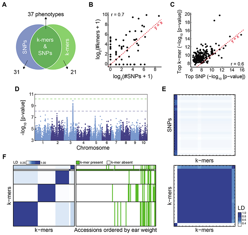
To demonstrate the usefulness of our approach with larger, more complex genomes, we turned to maize²⁴, a species with a ~2.5 Gb genome and extensive presence/absence variation of genes^10,25,26. We applied our approach to 252, mostly morphological, traits²⁷ in 150 inbred lines with short read sequence coverage of at least 6x²⁸. A total of 2.3 billion k-mers were present in at least five accessions (Extended Data Fig. 8A). For 89 traits, significant associations were identified by at least one of the methods, and for 37 by both (Fig. 4A). As in A. thaliana, statistically significant variants as well as top associations were well correlated between both methods (Fig. 4B,C, Extended Data Fig. 8B-D). Top k-mers had lower p-values than top SNPs (Extended Data Fig. 8E), and the k-mer method detected associations not found by SNPs.

Figure 4. SNP- and k-mer-based GWAS in maize.

(A) Overlap between SNP and k-mer hits. See also Extended Data Fig. 8B,C.

(B) Correlation of numbers of significant k-mers vs. SNPs. See also Extended Data Fig. 8E.

(C) Correlation of p-values of top k-mers and SNPs.

(D) SNP associations with days to tassel (environment 06FL1).

(E) LD between 23 significant SNPs and 18 k-mers (top) or k-mers to k-mers (bottom) for days to tassel. Order of k-mers is the same in both heatmaps.

(F) LD between 45 k-mers associated with ear weight (environment 07A, left), and k-mer presence/absence patterns in different accessions ordered by their ear weight (right).

A major challenge for maize is the high fraction of short reads that do not map uniquely to the genome. Previously, additional information had to be used to find the genomic position of SNPs, including population LD and genetic map position²⁸. We therefore compared SNPs and k-mers using LD, without locating k-mers in the genome. In several cases, a k-mer marked a common allele in the population with strong phenotypic effects, without the allele having been identified with SNPs. For example, for days-to-tassel, one clear SNP hit was also tagged by k-mers (Fig. 4D,E), but a second variant was only identified with k-mers. Another example was ear weight for which no SNP (Extended Data Fig. 8F), but several unlinked k-mer-tagged variants were identified (Fig. 4F). Thus, new alleles with high predictive power for maize traits can be revealed using k-mers.

As with SNPs, the difficulty of unique short read mappings also undermined the ability to identify the source of k-mers associated with specific traits. For example, we tried to locate the genomic position of the k-mer corresponding to the SNP associated with days-to-tassel in chromosome 3 (Fig. 4D). Only about 1% of reads from which the k-mers originated could be mapped uniquely to the reference genome. However, when we assembled all these reads into a 924 bp contig, we could place it to the same place as the identified SNPs. This fragment had two single-base pair differences relative to the reference genome, and was not in the proximity of any gene. Thus, we could use the richness of combining reads from several accessions to more precisely locate the variant origin.

k-mer-based GWAS in tomato

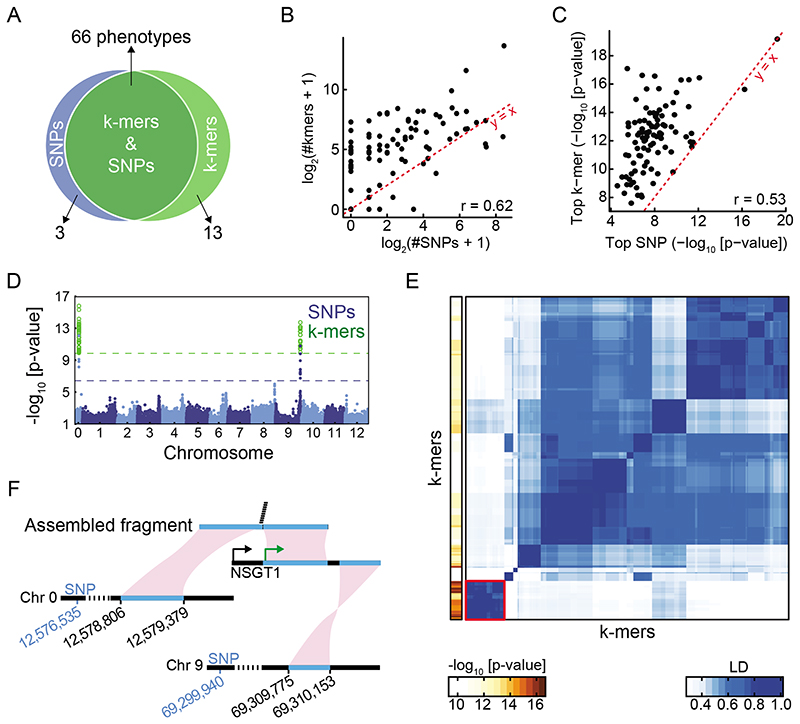
At ~900 Mb, the tomato genome is smaller than that of maize, but it presents its own challenges, as there is a complex history of introgressions from wild relatives into domesticated tomatoes^29,30. Starting with 981 million k-mers from 246 accessions (Extended Data Fig. 9A), we performed GWA on 96 metabolites measurements^31,32. For many metabolites, an association was identified by both methods, but three had only SNP hits and 13 only k-mer hits (Fig. 5A). Similar to the other species, the number of identified variants as well as top p-values were correlated between methods (Fig. 5B,C). Top k-mer associations were also stronger than top SNPs (Extended Data Fig. 9D), even more so than in A. thaliana or maize.

Figure 5. SNP- and k-mer-based GWAS in tomato.

(A) Overlap between SNP and k-mer hits. See also Extended Data Fig. 9B,C.

(B) Correlation of numbers of significant k-mers vs. SNPs. See also Extended Data Fig. 9E.

(C) Correlation of p-values of top k-mers and SNPs.

(D) SNP and k-mer associations with guaiacol concentration.

(E) LD among 293 k-mers associated with guaiacol concentration (right), and the p-value of each k-mer (left). Red square on bottom left indicates the 35 k-mers with lowest p-values and no mappings to the reference genome.

(F) Part of a fragment assembled from the 35 unmapped k-mers (E) mapped to chromosome 0 and another part to the unanchored complete NSGT1 gene from a non-reference accession. Only the 3’ end of NSGT1 is found in the reference genome, on chromosome 9. The green and black arrows mark the start of the NSGT1 ORF in the R104 “smoky” line and “non-smoky” lines³³. The two significant SNPs closest to the two regions in the reference genome are indicated in blue.

As a case study, we studied the concentration of guaiacol, responsible for a strong off-flavor in tomato³¹. Associated SNPs were found in chromosome 9 and what is called “chromosome 0” (Fig. 5D), which contains sequence scaffolds not assigned to the 12 nuclear chromosomes. From the 293 guaiacol associated k-mers, 180 could be mapped uniquely to the genome, all close to significant SNPs. Among the remaining k-mers, of particular interest was a group of 35 k-mers in high LD and with especially low p-values (Fig. 5E). Assembly of the corresponding short reads resulted in a 1,172 bp fragment, of which the first 574 bp aligned near significant SNPs in chromosome 0 (Fig. 5F), and the remainder matching the non-reference NON-SMOKY GLYCOSYLTRANSFERASE 1 (NSGT1) gene, which had been originally pinpointed as causal for variation in guaiacol³³. The 35 significant k-mers covered the junction between these two mappable regions. Most of the NSGT1 coding sequence is absent from the reference genome, but present in other accessions. The significant SNPs identified in chromosomes 0 and 9 apparently represent the same region in other accessions, connected by the fragment we assembled (Fig. 5F). Thus, we identified an association outside the reference genome, and linked the SNPs in chromosome 0 to chromosome 9.

k-mer based kinship estimates

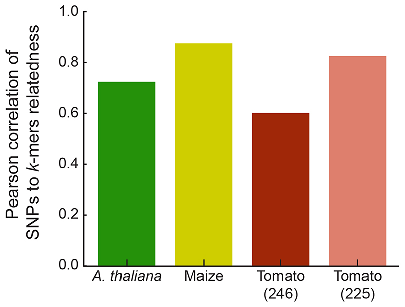
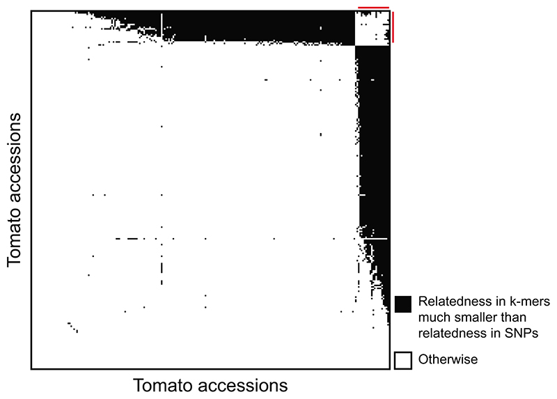
We have shown that one can assemble short fragments from k-mer-containing short reads and find hits not only in the reference genome, but also in other published sequences. This opens the possibility to apply our method to species without a high-quality reference genome, since contigs that include multiple genes can be relatively easily and cheaply generated³⁴. The major question with such an approach is then how to correct for population structure in the GWA step without kinship information from SNPs, determined by mapping to a reference genome. To learn kinship directly from k-mers, we estimated relatedness using k-mers, with presence/absence as the two alleles. We calculated the relatedness matrices for A. thaliana, maize, and tomato and compared them to the SNP-based relatedness. In all three species there was agreement between the two methods, although initial results were clearly better for A. thaliana and maize than for tomato (Fig. 6). The inferior performance in tomato was due to 21 accessions (Extended Data Fig. 10), that appeared to be more distantly related to the other accessions based on k-mers than what had been estimated with SNPs. This is likely due to these accessions containing diverged genomic regions that perform poorly in SNP calling, resulting in inaccurate relatedness estimates. In conclusion, k-mers can be used to calculate relatedness between individuals, thus paving the way for GWAS in organisms without high-quality reference genomes.

Figure 6. Kinship matrix estimates with k-mers.

Relatedness between accessions was independently estimated based on SNPs and k-mers. The correlation between the two for tomato could be improved by removing 21 accessions (Extended Data Fig. 10).

Discussion

The complexity of plant genomes can make SNP-based identification of genotype-phenotype associations challenging. We have shown that k-mers can not only identify almost all associations found by SNPs and short indels, but also SVs and variants in sequences not present in reference genomes. The expansion of variant types detected by the k-mer method complements SNP-based approaches, and increases opportunities for finding and exploiting complex genetic variants driving phenotypic differences in plants regardless of reference genome quality.

k-mers mark genetic polymorphisms in the population, but the types and genomic positions of these polymorphisms are initially not known. While one can also use k-mers for predictive models without knowing their genomic context, in many cases the genomic context of associated k-mers is of interest. The simplest solution is to align k-mers or the corresponding short reads to a reference genome³⁵. More interesting are cases where k-mers cannot be placed on the reference genome. For these, one can first identify the originating short reads and assemble these into larger fragments, which is a very effective path to uncovering the genomic context of k-mers. The resulting fragment also captures phased haplotype information. Combining reads from multiple accessions can provide high local coverage around k-mers of interest, increasing the chances that sizeable fragments can be assembled and located.

A further improvement will be the use of k-mers to tag heterozygous variants. In our current implementation, which relies on presence/absence of k-mers, one of the homozygous states has to be clearly differentiated not only from the alternative homozygous state, but also from the heterozygous state. This did not affect comparisons between SNPs and k-mers in this study, as we only looked at inbred populations, where only homozygous, binary states are expected. Another improvement will be the use of k-mers to detect causal copy number variations. So far, we can only tag copy number variants if the junctions produce unique k-mers, but it would be desirable to use also k-mers inside copy number variants. Normalized k-mer counts would create a framework that could, at least in principle, detect almost any kind of genomic variation.

The comparison of k-mer- and SNP- based GWAS provides an interesting view on tradeoffs in the characterization of genetic variability. The lower top p-values obtained with k-mers where a SNP is the underling variant suggest incomplete use of existing information in SNP calling. On the other hand, our analysis likely included some k-mers that represent only sequencing errors. While requiring k-mers to appear multiple times in a sequencing library and in multiple individuals removes most sequencing errors, this can also lead to some k-mers being labeled erroneously as absent. Finally, there is the increase in test load, an inevitable result of increasing the search space to tag more genetic variants.

k-mers invert how GWAS is usually done. Instead of first locating sequence variations in the genome, we begin with sequence-phenotype associations and only then find the genomic context of associated sequences. Technological improvement in short- and long-read sequences as well as methods to integrate them into a population-level genetic variation data-structure will expand the covered genetic variants^36,37. While traditional GWAS methods will benefit from these technological improvements, so will k-mer-based approaches, which will be able to use tags spanning larger genomic distances. Therefore, we posit that for GWAS purposes, k-mer based approaches are ideal because they minimize arbitrary choices when classifying alleles and because they capture more, almost optimal, information from raw sequencing data.

Methods

Curation of an A. thaliana phenotype compendium

Studies containing phenotypic data on A. thaliana accessions were located by searching NCBI PubMed using a set of general terms. For most studies, relevant data was obtained from the supplementary information. Otherwise, requests were sent to the corresponding authors. Data already uploaded to the AraPheno dataset³⁸ was downloaded from there. Phenotypic data in PDF format was extracted using Tabula software. Different sets of naming for accessions were converted to accession indices. In case an index for an accession could not be located, we omitted the corresponding data point. In case an accession could potentially be assigned to different indices, we first checked if it was part of the 1001 Genomes project; if so, we used the 1001 Genomes index. In case the accession was not part of it, one of the possible indices was assigned at random. Phenotypes of metabolite measurements from two studies^39,40, were filtered to a reduced set by the following procedure: take the first phenotype, sequentially retain phenotypes if correlation with all previously taken phenotypes is lower than 0.7. Data from the second study⁴⁰, were further filtered for phenotypes with a title. Assignment of categories for each phenotype was done manually (Supplementary Table 1). All processed phenotypic data can be found in https://zenodo.org/record/3701176#.XmX9u5NKhhE

Whole genome sequencing data and variant calls of A. thaliana

Whole genome short reads for 1,135 A. thaliana accessions were downloaded from NCBI SRA (accession SRP056687). Accessions with fewer than 10⁸ unique k-mers, a proxy for low effective coverage, were removed, resulting in a set of 1,008 accessions. The 1001 Genomes project VCF file with SNPs and short indels was downloaded from http://1001genomes.org/data/GMI-MPI/releases/v3.1 and condensed into these 1,008 accessions, using vcftools v0.1.15⁴¹. We required a minor allele count (MAC) of 5 individuals, resulting in 5,649,128 genetic variants. The VCF file was then converted to a PLINK binary file using PLINK v1.9⁴². The TAIR10 reference genome was used for short read and k-mer alignments. Coordinates for genes in figures were taken from Araport11⁴³.

Whole genome sequencing data and variant calls of maize

Whole genome short reads of maize accessions corresponded to the “282 set” part of the maize HapMap3.2.1 project²⁸. Sequencing libraries “x2” and “x4” were downloaded from NCBI SRA (accession PRJNA389800) and combined. Coverage per accession was calculated as number of reads multiplied by read length and divided by the genome size, data for 150 accessions with coverage >6x was used. Phenotypic data for 252 traits measured for these accessions were downloaded from Panzea²⁷.

Two of these phenotypes were constant over more than 90% of the 150 accessions, these two were removed from further analysis (“NumberofTilleringPlants_env_07A”, “TilleringIndex-BorderPlant_env_07A”). The HapMap3.2.1 VCF files (c*_282_corrected_onHmp321.vcf.gz) of SNPs and indels were downloaded from Cyverse. Variant files were filtered using vcftools v0.1.15 to the relevant 150 accessions. Variants were further filtered for MAC of ≥5, resulting in a final set of 35,522,659 variants. The B73 reference genome, version AGPv3⁴⁴, that was used to create the VCF file, was downloaded from MaizeGDB and used for alignments⁴⁴.

Whole genome sequencing data and variant calls of tomato

Whole genome short reads were downloaded for 246 accessions with coverage >6x, from NCBI SRA and EBI ENA (accession numbers SRP045767, PRJEB5235 and PRJNA353161). A table with coverage per accession was shared by the authors³¹. Metabolite measurements were taken from Tieman et al.³¹ (only adjusted values) and a subset of metabolites from Zhu et al.³². These were filtered to a reduced set by the following procedure: take the first phenotype, sequentially retain phenotypes if correlation with all previously taken phenotypes is lower than 0.7. Metabolites were ordered as reported originally³². Only one repeat, the one with more data points and requiring at least 40 data points was retained. The VCF file with SNPs and short indels³¹ was obtained from the authors and filtered for the relevant 246 accessions. Variants were further filtered for MAC of ≥5, resulting in a final set of 2,076,690 variants. Reference genome SL2.5²⁹ (https://www.ncbi.nlm.nih.gov/assembly/GCF_000188115.3/) used to create the VCF file was used for alignments.

Calculate and comparison of kinship matrices

Kinship matrix of relatedness between accessions was calculated as in EMMA⁴⁶, with default parameters. The algorithm was re-coded in C++ to read directly PLINK binary files. For k-mers based relatedness the same algorithm was used, coding presence/absence as two alleles. For comparison of k-mers- to SNPs-based relatedness we correlated (Pearson) the values for all $\frac{n}{2}$ pairs, for n accessions. For tomato, 3492 pairs had a relatedness more than 0.15 lower for k-mer than for SNPs. 3,298 (94.4%) of these pairs were between a set of 21 accessions and all other 225 accessions. We calculated the correlation twice: for all pairs, and only between pairs of these 225 accessions.

GWA on SNPs and short indels or on full k-mers table

Genome-wide association on the full set of SNPs and short indels was conducted using linear mixed models with the kinship matrix, using GEMMA version 0.96¹⁴. Minor allele frequency (MAF) was set to 5% and MAC was set to 5, with a maximum of 50% missing values (-miss 0.5). To run GWA on the full set of k-mers (e.g. in Fig. 1B), k-mers were first filtered for k-mers having only unique presence/absence patterns on the relevant set of accessions, MAF of at least 5%, and MAC of at least 5. Presence/absence patterns were then condensed to only the relevant accessions and output as a PLINK binary file directly. GEMMA was then run using the same parameters as for the SNPs GWA described above.

Phenotype covariance matrix estimation and phenotypes permutation

EMMA (emma.REMLE function) was used to calculate the variance components which were used to calculate the phenotypic covariance matrix⁴⁶. We then calculated 100 permutations of the phenotype using the mvnpermute R package¹⁵. The n% (e.g. n=5 gives 5%) family-wise error rate threshold was defined by taking the n^th top p-value from the 100 top p-values of running GWA on each permutation. In all cases, unless indicated otherwise, the 5% threshold was used.

Scoring p-values from GWA for similarity to uniform distribution and filtering phenotypes

Each SNP-based GWA run was scored for a general bias in p-value distribution, similar to Atwell et al.⁴⁷. All SNPs p-values were collected, the 99% higher p-values were tested against the uniform distribution using a kolmogorov-smirnov test, and the test statistic was used to filter phenotypes for which distribution deviated significantly from the uniform distribution. A threshold of 0.05 was used, filtering 89, 0, and 295 phenotypes for A. thaliana, maize and tomato, respectively.

k-mer GWA

Association of k-mers was done in two steps, with the aim of getting the most significant k-mers p-values. The first step was based on the approach used in Bolt-lmm-inf or GRAMMAR-Gamma^16,17. For phenotypes y, genotypes g, and a covariance matrix Ω, the k-mer score is:

$$T_{score}^2=\frac{1}{\gamma }\frac{{\left({\tilde{g}}^T{\Omega }^{-1}\tilde{y}\right)}^2}{{\tilde{g}}^T\tilde{g}}$$

Where $\tilde{g}=g-E(g)$ and $\tilde{y}=y-E(y)$. The first step was used only to filter a fixed number of top k-mers, thus we could use any score monotonous with $T_{\text{score} }^2$ and specifically $\frac{{\left({\tilde{g}}^T{\Omega }^{-1}\tilde{y}\right)}^2}{{\tilde{g}}^T\tilde{g}}$ which is independent of γ (see supplementary note on calculation optimization and Supplementary Table 3). In the second step, the best k-mers were run using GEMMA to calculate the likelihood ratio test p-values¹⁴.

The number of k-mers filter in the first step was set to 10,000 for A. thaliana and 100,000 for maize and tomato. Both steps associate k-mers while accounting for population structure, while the first step uses an approximation, the second use an exact model. Therefore, real top k-mers might be lost as they would not pass the first filtering step. To control for this, we first defined the 5% family-wise error-rate threshold based on the phenotype permutations, and then identified all the k-mers which passed the threshold. Next, we used the following criteria to minimize the chance of losing k-mers: we checked if all identified k-mers were in the top N/2 k-mers from the ordering of the first step (N=10,000 or 100,000 dependent on species). For example, in maize all k-mers passing the threshold in the second step should be in the top 50,000 k-mers from the first step. The probability that this will happen randomly is 2 ^-m, where m is number of identified k-mers, in most phenotypes this is very unlikely. In 8.5% of phenotypes from A. thaliana the criteria was not fulfilled, for these phenotypes we re-run the two-steps with 100x more k-mers filtered in the first step, that is 1,000,000 k-mers. For 6 phenotypes the criteria still did not hold, these phenotypes were not used in further analysis. In tomato, 33% of phenotypes did not fulfill these criteria, in these cases we re-run the first step with 100x more k-mers filtered (10,000,000), 17 phenotypes still did not pass the threshold and were omitted from further analysis. The permutations were not re-run, and the threshold defined using 100,000 k-mers was used, as the top k-mer used to define the threshold tended to be high in the list. For maize all phenotypes passed the criteria and no re-running was needed.

SNP-based GWAS on phenotype permutations

To calculate thresholds for SNPs-based GWAS we used the two step approach used for k-mers. The permuted phenotypes were run in two steps as we were only interested in the top p-value to define thresholds. We filtered 10,000 variants in the first step which were then run using GEMMA to get exact scores¹⁴. The non-permuted phenotype were run using GEMMA on all the variants.

Calculation of linkage-disequilibrium (LD)

For two variants, x and y, each can be a k-mer or a SNP, LD measure was calculated using the r² measure⁴⁸. For a k-mer, variants were coded as 0/1, if absent or present, respectively. For SNPs one variant was coded as 0 and the other as 1. If one of the variants had a missing or heterozygous value in a position, this position was not used in the analysis. The LD value was calculated using the formula:

$$r^2=\frac{{(p(x=1\&y=1)-p(x=1)\ast p(y=1))}^2}{p(x=1)\ast p(y=1)\ast p(x=0)\ast p(y=0)}$$

Comparing Col-0 and Ler genome assemblies with k-mers

The list of 31 bp k-mers that are part of the Col-0 TAIR10 and the Ler genomes²² were created using KMC v3⁴⁵. The k-mer lists from the two genomes were filtered for: k-mers appearing in a single genome and ones appearing only once in a genome. The positions of the filtered k-mers were identified by checking each position in the genome against the filtered lists. In Extended Data Fig. 1, k-mers from these lists are plotted around four variants, defined previously²². The statistics presented in Extended Data Fig. 2 are for all variants reported in Supplementary Tables of Zapata and colleagues²², under the titles: “Lindel_Allelic”, “Lindel_NonAllelic”, “IntraChromTransloc”, “InterChromTransloc”, and “InversionSites”.

Calculating LD of closest SNP/k-mer (Supplementary Figure 1)

To calculate LD between all k-mers and all SNPs in the A. thaliana 1001 Genomes Project (1001G) collection, the 1001G imputed SNPs matrix was used⁴⁹ (provided by Ümit Seren), to avoid dealing with missing values present in the original VCF file. The imputed matrix was condensed to the 1,008 accessions used in the k-mers table, and only SNPs with MAF ≥ 0.05 were considered. k-mers were also filtered for MAF ≥ 0.05. We were left with 898,869 SNPs and 163,644,699 k-mers, therefore the complexity of calculating all LD is: (898,869)x(163,644,699)x(1,008) ≥ 10¹⁷. This calculation was done using the SSE4 command set, by representing the variant per individual as one bit and combining 64 individuals in one CPU word. Only maximal LD of each SNP to all k-mers and of each k-mer to all SNPs were saved.

LD cumulative graph (Figure 2E,H)

For a set of phenotypes and for every l=0,0.05,..,1 we calculated the percentage of phenotypes for which exists a k-mer or a SNP in the pre-defined group which is in LD ≥ l with top SNP or top k-mer, respectively. The pre-defined groups are: (1) all the k-mers which passed the SNPs defined threshold in Figure 2E or (2) all the SNPs or k-mers which passed their own defined thresholds in Figure 2H. The percentage is then plotted as a function of l.

Retrieving source reads of a specific k-mer and assembling them

For a k-mer identified as being associated with a phenotype we first looked in the k-mers-table and identified all accessions taking part in the association analysis and having this k-mer present. For each of these accessions we went over all sequencing reads and filtered out all paired-end reads which contained the k-mer. To assemble paired-reads, SPAdes v3.11.1 was used with “--careful” parameter⁵⁰.

Alignment of reads or k-mers to the genome

Paired-end reads were aligned to the genome using bowtie2 v2.2.3, with the “--very-sensitive-local” parameter. k-mers were aligned to the genome using bowtie v1.2.2 with “--best --all --strata” parameters⁵¹.

Analysis of flowering time in 10C (Figure 1, Extended Data Fig. 5)

To find the location in the genome of the 105 identified k-mers, k-mers were first mapped to the A. thaliana genome. 84 of the k-mers had a unique mapping, one was mapped to multiple locations and 20 could not be mapped. For the 21 k-mers with no unique mapping we located the sequencing reads they originated from, and mapped the reads to the A. thaliana genome. For each of the k-mers we looked only on the reads with the top mapping scores. For the one k-mer which had multiple possible alignment also the originating reads did not have a consensus mapping location in the genome. For every k-mer from the 20 non-mapped k-mers, all top reads per k-mer, in some cases except one, mapped to a specific region spanning a few hundred base pairs. The middle of this region was defined as the k-mer position for the Manhattan plot in Figure 1D. To find the locations of all k-mers presented in Extended Data Fig. 5D, we used only uniquely uniquely k-mers.

To find the location of the 93 associated k-mers of length 25 bp, presented in supplementary Extended Data Fig. 5E, we followed the same procedure: 87 k-mers had unique mapping, one mapped multiple times and 5 could not be mapped. For the 5 non-mappable k-mers and the k-mer with non-unique mapping, we located the originated short reads and aligned them to the genome. For each of the 5 k-mers all reads with top mapping score mapped to a specific region of a few hundred base pairs, we took the middle of the region as the location in the Manhattan plot. For the k-mer with multiple mappings, 15 out of the 17 reads mapped to the same region and we used this location. All k-mers mapped to the 4 location in the genome for which SNPs were identified except one - AAGCTACTTGGTTGATAATACTAAT. The reads from which this k-mer originated mapped to the same region in chromosome 5 position 3191745-3192193 and we used the middle of this region.

Analysis of xylosides fraction (Figure 3A,B and Extended Data Fig. 7B,C)

All k-mers passing the threshold, were mapped uniquely to chromosome 5 in the region 871,976 – 886,983. Of the 123 identified k-mers, 27 had the same minimal p-value (−log10(p−value) =44.7). These k-mers mapped to chromosome 5 in positions 871,976-872,002, all covering the region 872,002-872,007. For the 60 accessions used in this analysis, all reads from the 1001G were mapped to the reference genome. The mapping in region 872,002-872,007 of chromosome 5 were examined manually by IGV in all accessions⁵², and the 2 SNPs 872,003 and 872,007 were called manually without knowledge of the phenotype value.

The hierarchical clustering in Extended Data Fig. 7B was done according to all SNPs in chromosome 5 from position 870,000 to 874,000. The distance between two accessions is the average number of SNPs with different values taking into account only no missing values.

Analysis of growth inhibition in presence of flg22 (Figure 3C,D)

The phenotype in the original study was labeled “flgPsHRp”¹⁹. For each of the 7 k-mers which could not be mapped uniquely to the genome, the originated reads from all accessions were retrieved and assembled. All the seven cases resulted in the same assembled fragment (SEQ1, Supplementary Table 2). Using NCBI BLAST we mapped this fragment to chromosome 1: position 40-265 were mapped to 8169229-8169455 and position 262-604 were mapped to 8170348-8170687. For every accession from the 106 that were used in the GWAS analysis we tried to locally assemble this region, to see if the junction between chromosome 1 positions 8169455-8170348 could be identified. We used all the 31 bp k-mers from the above assembled fragment as bait, and located all the reads for each accession separately. For 11 out of the 13 accessions that had all 10 identified k-mers we got a fragment from the assembly process. In all 11 cases the exact same junction was identified. For 1 of the 4 accessions that had only part of the 10 identified k-mer we got a fragment from the assembler, which had the same junction. For 43 of the 89 accessions that had none of the identified k-mers the assembly process resulted in a fragment, in none of these cases the above junction could be identified.

Analysis of germination in darkness and low nutrients (Figure 3E, F)

The phenotype in the original study was labeled “k_light_0_nutrient_0”²¹. The 11 identified k-mers had two possible presence/absence patterns, separating them into two groups of 4 and 7 k-mers. The short-read sequences containing the 4 or 7 k-mers were collected separately and assembled, resulting in the exact same 458bp fragment (SEQ2, Supplementary Table 2). This fragment was used as a query in NCBI BLAST search, resulting in alignment to Ler-0 chromosome 3 (LR215054.1) positions 15969670-15970128. The region between (15969670-3000) to (15970128+3000) in LR215054.1 was retrieved and used as query to a NCBI BLAST search. The fragment mapped to Col-0 reference genome chromosome 3 (CP002686.1). Region 1-604 to 16075369-16075968, region 930-1445 to 16076025-16076532, region 3446-3946 to 16079744-16080244, and region 3958-6459 to 16080301-16082781.

Analysis of root branching zone (Supplementary Figure 2)

The phenotype in the original study was labeled “Mean(R)_C”, that is Branching zone in no treatment⁵³. No SNPs and 1 k-mer (AGCTACTTTGCCACCCACTGCTACTAACTCG) passed their corresponding 5% thresholds. The k-mer mapped the chloroplast genome in position 40297, with 1 mismatch. No SNPs and another k-mer (CCGGCGATTACTAGAGATTCCGGCTTCATGC) passed the 10% family-wise error-rate threshold. This k-mer mapped non-uniquely to two place in the chloroplast genome: 102285 and 136332.

Analysis of Lesion by Botrytis cinerea UKRazz (Extended Data Fig. 7A)

The Lesion by Botrytis cinerea UKRazz phenotype was labeled as “Lesion_redgrn_m_theta_UKRazz”. In the GWA analysis 19 k-mers and no SNPs were identified. All k-mers had the same presence/absence pattern. The short-read sequences from which the k-mers originated were mapped to chromosome 3 around position 72,000bp, and contained a 1-bp deletion of a T nucleotide in position 72,017. Whole genome sequencing reads were mapped to the genome for the 61 accessions with phenotypes used in these analyses. We manually observed the alignment around position 72,017 of chromosome 3, without the prior knowledge if the accession had the identified k-mers. For 20 accessions, we observed the 1-bp deletion in position 72,017, all 19 accessions containing the k-mers were part of these 20.

Analysis of days-to-tassel and ear weight in maize (Figure 4)

Ear weight phenotype was labeled “EarWeight_env_07A” in original dataset²⁷. Days to tassel were measured in growing degree days (GDD) and was labeled as “GDDDaystoTassel_env_06FL1” in original dataset. In comparison of LD between k-mers and SNPs in days to tassel (Fig. 4E, upper panel), two SNPs were filtered out as having more than 10% heterozygosity and one as having, exactly, 50% missing values. In days to tassel the k-mer which was similar to identified SNPs was AGAAGATATCTTATGAACTCCTCACCAGTAA. The 171 paired-end reads from which this k-mer originated mapped to the genome as follows - 2 (1.17%) aligned concordantly 0 times, 2 (1.17%) aligned concordantly exactly 1 time, and 167 (97.66%) aligned concordantly >1 times. The assembly of these reads produce two fragments, the first of length 273bp with coverage of 1.23 and the second of length 924bp and with coverage of 27.41 (SEQ3, Supplementary Table 2). We aligned this second fragment to the genome using Minimap2, with the default parameters⁵⁴. Minimap2 reported only 1 hit to chromosome 3 (NC_024461.1) in positions 159141222-159142137.

Analysis of guaiacol concentration in tomato (Figure 5D-F)

Guaiacol concentration was labeled “log3_guaiacol” in the original study. From the 293 k-mers passing the threshold, 184 could be mapped uniquely to the genome: 135 to chromosome 0 between position 12573795-12576534, and 45 to chromosome 9 between position 69301436-69305717, 3 to chromosome 6 between position 8476136-8476138, and 1 to chromosome 4 at position 53222324. The 4 k-mers mapped to chromosome 4 and 6 were checked manually by locating the reads containing them and aligning the reads to the genome, in all cases no reads were able to be aligned to the genome (>99.5% of reads). For the 35 k-mers not mapping to genome and in high LD, visualized in Figure 5E, all reads containing at least one of the k-mers were retrieved and assembled (SEQ4, Supplementary Table 2). NCBI Blast search of this fragment resulted in: positions 1-574 mapped to positions: 12578806-12579379 in chromosome 0 of the tomato genome (CP023756.1) and positions 580-1169 mapped to positions 289-878 in NSGT1 (KC696865.1). The R104 “smoky” accession NSGT1 ORF starts at position 307, as reported previously³³. NCBI BLAST of NSGT1 (KC696865.1), identified mapping to chromosome 9 of the tomato genome (CP023765.1), from positions 975-1353 to positions 69310153-69309775.

Extended Data

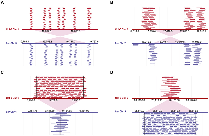
Extended Data Fig. 1. Examples of well characterized structural variant tagged by k-mers.

Examples of how k-mers tag well characterized structural variants²² between the Col-0 reference genome and the Ler fully assembled genome. The two genomes were used to count 31 bp k-mers, and all k-mers unique to one genome and appearing only once in it were plotted in the indicated regions. The (A) translocation, (B) inversion and (C-D) insertion/deletion positions are indicated by vertical lines and red shades. The k-mers unique to Col-0/Ler are plotted in the upper/lower panels in red/blue, respectively. The five positions tagged by k-mers inside the translocation presented in (A) are either SNPs or 1 bp indels.

Extended Data Fig. 2. Genome-wide evaluation of k-mer potential to detect SVs in well-characterized genomes.

(A) For every translocation or inversion, previously identified²² between the Col-0 reference genome or the Ler genome we evaluate if it is tagged by 31 bp k-mers. Each translocation or inversion will affect 4 edges between the translocated fragment and the neighbouring genomic regions (bottom panel). For every previously identified translocation or inversion, the number of edges (0-4) which are tagged by k-mers unique to one genome were counted. Only 1.1% of these SVs were not tagged by any k-mer unique to one genome (upper panel).

(B) For every edge tagged by k-mers, described in A, we plot the number of k-mers unique to one genome which tagged it. The histogram is enriched with edges covered by the maximal number of k-mers, 31.

(C) Evaluating the potential to tag by k-mers long insertions/ deletions between the well characterized genomes of Col-0 and Ler²². While in the genome with the apparent deletion only the junction between the two fragments will be tagged by unique k-mers, in the genome with the apparent insertion, the entire insert will be tagged (bottom panel). Only 0.4% of the previously characterized long insertions/deletions are not tagged by unique k-mers.

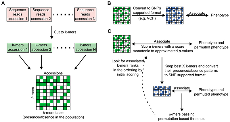
Extended Data Fig. 3. Pipeline for k-mer-based GWAS.

(A) Creating the k-mer presence/absence table: Each accession’s genomic DNA sequencing reads are cut into k-mers⁴⁵, filtering k-mers appearing less than twice/thrice in a sequencing library. k-mers are further filtered to retain only those present in at least 5 accessions, and ones that are found in both forward and reverse-complement form in at least 20% of accessions they appeared in. All k-mer lists are combined into a k-mer presence/absence table.

(B) Genome-wide associations on the full k-mers table using SNP-based software: the k-mers table is converted into PLINK binary format, which is used as input for SNP-based association mapping software^14,42.

(C) GWA optimized for the k-mers: k-mers presence/absence patterns are first associated with the phenotype and its permutations using a LMM to account for population structure^16,17. This first step is done by calculating an approximated score of the exact model. Best k-mers from this first step (e.g. 100,000 k-mers) are passed to the second step, In which an exact p-value is calculated¹⁴ for both the phenotype and its permutations. A permutation-based threshold is calculated, and all k-mers passing this threshold are checked for their rank in the scoring from the first step. If not all k-mers hits are in the top 50% of the initial scoring, then the entire process is rerun from the beginning, passing more k-mers from the first to the second step. This last test is built to confirm that the approximation of the first step will not remove true associated k-mers.

Extended Data Fig. 4. Allele counts for A. thaliana 1001G k-mers.

Histogram of k-mer allele counts: For every N=1..1008, the number of k-mers appeared in exactly N accessions is plotted.

Extended Data Fig. 5. Flowering time-genotype associations in A. thaliana identified with k-mers.

(A) LD between SNPs associated with flowering time. Dashed lines represent the four variant types, as in Figure 1C.

(B) LD between k-mers associated with flowering time, Dashed lines represent the four variant types, as in Figure 1C.

(C) Same as Figure 1D with only SNPs.

(D) Same as Figure 1D with only k-mers presented, showing also k-mers lower than the threshold.

(E) Manhattan plot of SNPs and k-mer associations with flowering time in 10°C as in Figure 1D for k-mers of length 25 bp.

Extended Data Fig. 6. Comparison of SNP- and k-mer-GWAS on phenotypes from 104 studies on A. thaliana accessions.

(A) Histogram of the number of identified k-mers vs. identified SNPs (in log₂) for A. thaliana phenotypes. Only the 458 phenotypes with both variant types identified were used.

(B) Histogram of thresholds difference of k-mers vs. SNPs of all A. thaliana phenotypes. Thresholds were -log₁₀ transformed.

Extended Data Fig. 7. Specific case studies in which k-mers are superior to SNPs.

(A) Results from GWAS on measurements of lesions by Botrytis cinerea UKRazz strain³⁹. An example of k-mers having better hold on a short variant: 19 k-mers and no SNPs were identified, all k-mers in complete LD (top row). Sequence reads containing the k-mers mapped to chromosome 3, with a single T nucleotide deletion out of an eight T’s stretch, in position 72,017. Manual (middle) and the 1001G project (bottom) calls are shown. In the 1001G, 57 of 61 accessions contain missing values.

(B) Haplotypes around SNPs associated with xylosides concentrations are not correlated with this trait. All SNPs in positions 870,000 to 874,000 in chromosome 5 were hierarchically clustered (left panel, white mark missing values). The two identified SNPs are marked by arrows and a close-up of their state is shown (middle panel). Phenotypic values colored according to the two SNPs: TG blue, TT red, and CT green (right panel).

(C-E) Manhattan plot for: (C) xyloside percentage, (D) seedling growth inhibition by a flg22 variant, (E) germination in darkness in low nutrient conditions.

(F) Germination phenotype plotted for accessions with top associated k-mer present or absent. Boxes cover 25%-75% percentiles, medians marked by horizontal lines, and whiskers cover the full range of values.

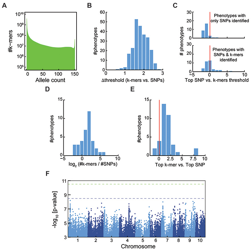
Extended Data Fig. 8. Comparison of SNP- and k-mer- based GWAS in maize.

(A) Histogram of k-mer allele counts for maize accessions.

(B) Histogram of difference between threshold values of SNPs and k-mers for maize phenotypes.

(C) Histogram of the top SNP p-value divided by the k-mers defined threshold, in (-log10), for maize phenotypes. Plotted for phenotypes with only identified SNPs (upper panel) or for phenotypes with both SNPs and k-mers identified (lower panel).

(D) Histogram of the number of identified k-mers vs. identified SNPs for maize phenotypes.

(E) Histogram of the difference between top (-log10) p-values in the two methods for maize phenotypes identified by both methods. Plotted as in Figure 2G.

(F) Manhattan plot of associations with ear weight (environment 07A). Associated k-mers could not be located in the reference genome, and are thus not presented.

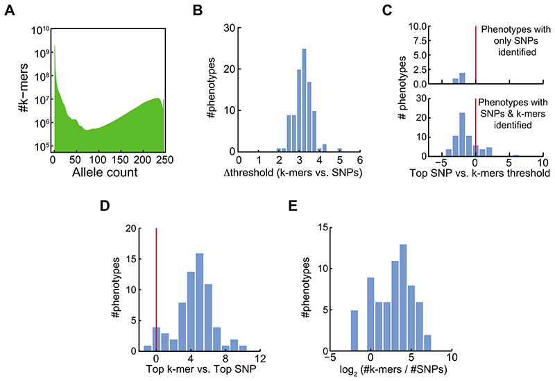
Extended Data Fig. 9. Comparison of SNP- and k-mer-based GWAS in tomato.

(A) Histogram of k-mers allele counts for tomato accessions.

(B) Histogram of difference between threshold values of SNPs and k-mers for tomato phenotypes.

(C) Histogram of the top SNP p-value divided by the k-mers defined threshold, in -log10, for tomato phenotypes. Plotted for phenotypes with only identified SNPs (upper panel) or for phenotypes with both SNPs and k-mers identified (lower panel).

(D) Histogram of the difference between top (-log10) p-values in the two methods for tomato phenotypes.

(E) Histogram of the number of identified k-mers vs. identified SNPs for tomato phenotypes.

Extended Data Fig. 10. Kinship matrix calculation based on k-mers for tomato accessions.

Identification of pairs of tomato accessions for which relatedness as measured with k-mers is much lower than relatedness as measured with SNPs. For every pair among the 246 accessions, a black square is plotted if the difference in relatedness between SNPs and k-mers is larger than 0.15. Accessions are ordered by the number of black square in their row/column. Red lines mark the 21 accessions with most black squares, that is, those for which the k-mer/SNP difference in relatedness is larger than 0.15 for the most pairs.

Data availability

A list of all phenotypes and top SNPs/k-mers passing their corresponding thresholds can be found here: https://zenodo.org/record/3701176#.XmX9u5NKhhE

The authors declare that all other data supporting the findings of this study are available within the supplementary information files.

Code availability

Code is available in https://github.com/voichek/kmersGWAS.

References

- 1.Saxena RK, Edwards D, Varshney RK. Structural variations in plant genomes. Brief Funct Genomics. 2014;13:296–307. doi: 10.1093/bfgp/elu016. [DOI] [PMC free article] [PubMed] [Google Scholar]
- 2.Iqbal Z, Caccamo M, Turner I, Flicek P, McVean G. De novo assembly and genotyping of variants using colored de Bruijn graphs. Nat Genet. 2012;44:226. doi: 10.1038/ng.1028. [DOI] [PMC free article] [PubMed] [Google Scholar]
- 3.Salzberg SL, Pertea M, Fahrner JA, Sobreira N. DIAMUND: direct comparison of genomes to detect mutations. Hum Mutat. 2014;35:283–288. doi: 10.1002/humu.22503. [DOI] [PMC free article] [PubMed] [Google Scholar]
- 4.Zielezinski A, et al. Benchmarking of alignment-free sequence comparison methods. Genome Biol. 2019;20:144. doi: 10.1186/s13059-019-1755-7. [DOI] [PMC free article] [PubMed] [Google Scholar]
- 5.Lees JA, et al. Sequence element enrichment analysis to determine the genetic basis of bacterial phenotypes. Nat Commun. 2016;7 doi: 10.1038/ncomms12797. 12797. [DOI] [PMC free article] [PubMed] [Google Scholar]
- 6.Sheppard SK, et al. Genome-wide association study identifies vitamin B5 biosynthesis as a host specificity factor in Campylobacter. Proc Natl Acad Sci U S A. 2013;110:11923–11927. doi: 10.1073/pnas.1305559110. [DOI] [PMC free article] [PubMed] [Google Scholar]
- 7.Lees JA, et al. Genome-wide identification of lineage and locus specific variation associated with pneumococcal carriage duration. eLife. 2017;6 doi: 10.7554/eLife.26255. [DOI] [PMC free article] [PubMed] [Google Scholar]
- 8.Rahman A, Hallgrímsdóttir I, Eisen M, Pachter L. Association mapping from sequencing reads using k-mers. Elife. 2018;7 doi: 10.7554/eLife.32920. [DOI] [PMC free article] [PubMed] [Google Scholar]
- 9.Gordon SP, et al. Extensive gene content variation in the Brachypodium distachyon pan-genome correlates with population structure. Nat Commun. 2017;8 doi: 10.1038/s41467-017-02292-8. 2184. [DOI] [PMC free article] [PubMed] [Google Scholar]
- 10.Sun S, et al. Extensive intraspecific gene order and gene structural variations between Mo17 and other maize genomes. Nat Genet. 2018;50:1289–1295. doi: 10.1038/s41588-018-0182-0. [DOI] [PubMed] [Google Scholar]
- 11.Minio A, Massonnet M, Figueroa-Balderas R, Castro A, Cantu D. Diploid Genome Assembly of the Wine Grape Carménère. G3. 2019;9:1331–1337. doi: 10.1534/g3.119.400030. [DOI] [PMC free article] [PubMed] [Google Scholar]
- 12.Arora S, et al. Resistance gene cloning from a wild crop relative by sequence capture and association genetics. Nat Biotechnol. 2019;37:139–143. doi: 10.1038/s41587-018-0007-9. [DOI] [PubMed] [Google Scholar]
- 13.1001 Genomes Consortium. 1,135 Genomes Reveal the Global Pattern of Polymorphism in Arabidopsis thaliana. Cell. 2016;166:481–491. doi: 10.1016/j.cell.2016.05.063. [DOI] [PMC free article] [PubMed] [Google Scholar]
- 14.Zhou X, Stephens M. Genome-wide efficient mixed-model analysis for association studies. Nat Genet. 2012;44:821–824. doi: 10.1038/ng.2310. [DOI] [PMC free article] [PubMed] [Google Scholar]
- 15.Abney M. Permutation testing in the presence of polygenic variation. Genet Epidemiol. 2015;39:249–258. doi: 10.1002/gepi.21893. [DOI] [PMC free article] [PubMed] [Google Scholar]
- 16.Svishcheva GR, Axenovich TI, Belonogova NM, van Duijn CM, Aulchenko YS. Rapid variance components-based method for whole-genome association analysis. Nat Genet. 2012;44:1166. doi: 10.1038/ng.2410. [DOI] [PubMed] [Google Scholar]
- 17.Loh P-R, et al. Efficient Bayesian mixed-model analysis increases association power in large cohorts. Nat Genet. 2015;47:284–290. doi: 10.1038/ng.3190. [DOI] [PMC free article] [PubMed] [Google Scholar]
- 18.Li X, et al. Exploiting natural variation of secondary metabolism identifies a gene controlling the glycosylation diversity of dihydroxybenzoic acids in Arabidopsis thaliana. Genetics. 2014;198:1267–1276. doi: 10.1534/genetics.114.168690. [DOI] [PMC free article] [PubMed] [Google Scholar]
- 19.Vetter M, Karasov TL, Bergelson J. Differentiation between MAMP Triggered Defenses in Arabidopsis thaliana. PLoS Genet. 2016;12 doi: 10.1371/journal.pgen.1006068. e1006068. [DOI] [PMC free article] [PubMed] [Google Scholar]
- 20.Bao W, Kojima KK, Kohany O. Repbase Update, a database of repetitive elements in eukaryotic genomes. Mob DNA. 2015;6:11. doi: 10.1186/s13100-015-0041-9. [DOI] [PMC free article] [PubMed] [Google Scholar]
- 21.Morrison GD, Linder CR. Association mapping of germination traits in Arabidopsis thaliana under light and nutrient treatments: searching for G×E effects. G3. 2014;4:1465–1478. doi: 10.1534/g3.114.012427. [DOI] [PMC free article] [PubMed] [Google Scholar]
- 22.Zapata L, et al. Chromosome-level assembly of Arabidopsis thaliana Ler reveals the extent of translocation and inversion polymorphisms. Proc Natl Acad Sci U S A. 2016;113:E4052–60. doi: 10.1073/pnas.1607532113. [DOI] [PMC free article] [PubMed] [Google Scholar]
- 23.Bryant FM, Hughes D, Hassani-Pak K, Eastmond PJ. Basic LEUCINE ZIPPER TRANSCRIPTION FACTOR67 Transactivates DELAY OF GERMINATION1 to Establish Primary Seed Dormancy in Arabidopsis. Plant Cell. 2019;31:1276–1288. doi: 10.1105/tpc.18.00892. [DOI] [PMC free article] [PubMed] [Google Scholar]
- 24.Schnable PS, et al. The B73 maize genome: complexity, diversity, and dynamics. Science. 2009;326:1112–1115. doi: 10.1126/science.1178534. [DOI] [PubMed] [Google Scholar]
- 25.Gore MA, et al. A first-generation haplotype map of maize. Science. 2009;326:1115–1117. doi: 10.1126/science.1177837. [DOI] [PubMed] [Google Scholar]
- 26.Springer NM, et al. The maize W22 genome provides a foundation for functional genomics and transposon biology. Nat Genet. 2018;50:1282–1288. doi: 10.1038/s41588-018-0158-0. [DOI] [PubMed] [Google Scholar]
- 27.Zhao W, et al. Panzea: a database and resource for molecular and functional diversity in the maize genome. Nucleic Acids Res. 2006;34:D752–7. doi: 10.1093/nar/gkj011. [DOI] [PMC free article] [PubMed] [Google Scholar]
- 28.Bukowski R, et al. Construction of the third-generation Zea mays haplotype map. Gigascience. 2018;7:1–12. doi: 10.1093/gigascience/gix134. [DOI] [PMC free article] [PubMed] [Google Scholar]
- 29.Tomato Genome Consortium. The tomato genome sequence provides insights into fleshy fruit evolution. Nature. 2012;485:635–641. doi: 10.1038/nature11119. [DOI] [PMC free article] [PubMed] [Google Scholar]
- 30.Lin T, et al. Genomic analyses provide insights into the history of tomato breeding. Nat Genet. 2014;46:1220–1226. doi: 10.1038/ng.3117. [DOI] [PubMed] [Google Scholar]
- 31.Tieman D, et al. A chemical genetic roadmap to improved tomato flavor. Science. 2017;355:391–394. doi: 10.1126/science.aal1556. [DOI] [PubMed] [Google Scholar]
- 32.Zhu G, et al. Rewiring of the Fruit Metabolome in Tomato Breeding. Cell. 2018;172:249–261. doi: 10.1016/j.cell.2017.12.019. e12. [DOI] [PubMed] [Google Scholar]
- 33.Tikunov YM, et al. Non-smoky glycosyltransferase1 prevents the release of smoky aroma from tomato fruit. Plant Cell. 2013;25:3067–3078. doi: 10.1105/tpc.113.114231. [DOI] [PMC free article] [PubMed] [Google Scholar]
- 34.Sohn J-I, Nam J-W. The present and future of de novo whole-genome assembly. Brief Bioinform. 2018;19:23–40. doi: 10.1093/bib/bbw096. [DOI] [PubMed] [Google Scholar]
- 35.Pascoe B, et al. Enhanced biofilm formation and multi-host transmission evolve from divergent genetic backgrounds in Campylobacter jejuni. Environ Microbiol. 2015;17:4779–4789. doi: 10.1111/1462-2920.13051. [DOI] [PMC free article] [PubMed] [Google Scholar]
- 36.Schneeberger K, et al. Simultaneous alignment of short reads against multiple genomes. Genome Biol. 2009;10 doi: 10.1186/gb-2009-10-9-r98. R98. [DOI] [PMC free article] [PubMed] [Google Scholar]
- 37.Paten B, Novak AM, Eizenga JM, Garrison E. Genome graphs and the evolution of genome inference. Genome Res. 2017;27:665–676. doi: 10.1101/gr.214155.116. [DOI] [PMC free article] [PubMed] [Google Scholar]
- 38.Seren Ü, et al. AraPheno: a public database for Arabidopsis thaliana phenotypes. Nucleic Acids Res. 2017;45:D1054–D1059. doi: 10.1093/nar/gkw986. [DOI] [PMC free article] [PubMed] [Google Scholar]
- 39.Fordyce RF, et al. Digital Imaging Combined with Genome-Wide Association Mapping Links Loci to Plant-Pathogen Interaction Traits. Plant Physiol. 2018;178:1406–1422. doi: 10.1104/pp.18.00851. [DOI] [PMC free article] [PubMed] [Google Scholar]
- 40.Chan EKF, Rowe HC, Hansen BG, Kliebenstein DJ. The complex genetic architecture of the metabolome. PLoS Genet. 2010;6 doi: 10.1371/journal.pgen.1001198. e1001198. [DOI] [PMC free article] [PubMed] [Google Scholar]
- 41.Danecek P, et al. The variant call format and VCFtools. Bioinformatics. 2011;27:2156–2158. doi: 10.1093/bioinformatics/btr330. [DOI] [PMC free article] [PubMed] [Google Scholar]
- 42.Purcell S, et al. PLINK: a tool set for whole-genome association and population-based linkage analyses. Am J Hum Genet. 2007;81:559–575. doi: 10.1086/519795. [DOI] [PMC free article] [PubMed] [Google Scholar]
- 43.Cheng C-Y, et al. Araport11: a complete reannotation of the Arabidopsis thaliana reference genome. Plant J. 2017;89:789–804. doi: 10.1111/tpj.13415. [DOI] [PubMed] [Google Scholar]
- 44.Portwood JL, et al. MaizeGDB 2018: the maize multi-genome genetics and genomics database. Nucleic Acids Res. (2nd) 2019;47:D1146–D1154. doi: 10.1093/nar/gky1046. [DOI] [PMC free article] [PubMed] [Google Scholar]
- 45.Kokot M, Dlugosz M, Deorowicz S. KMC 3: counting and manipulating k-mer statistics. Bioinformatics. 2017;33:2759–2761. doi: 10.1093/bioinformatics/btx304. [DOI] [PubMed] [Google Scholar]
- 46.Kang HM, et al. Efficient control of population structure in model organism association mapping. Genetics. 2008;178:1709–1723. doi: 10.1534/genetics.107.080101. [DOI] [PMC free article] [PubMed] [Google Scholar]
- 47.Atwell S, et al. Genome-wide association study of 107 phenotypes in Arabidopsis thaliana inbred lines. Nature. 2010;465:627–631. doi: 10.1038/nature08800. [DOI] [PMC free article] [PubMed] [Google Scholar]
- 48.Devlin B, Risch N. A comparison of linkage disequilibrium measures for fine-scale mapping. Genomics. 1995;29:311–322. doi: 10.1006/geno.1995.9003. [DOI] [PubMed] [Google Scholar]
- 49.Togninalli M, et al. The AraGWAS Catalog: a curated and standardized Arabidopsis thaliana GWAS catalog. Nucleic Acids Res. 2018;46:D1150–D1156. doi: 10.1093/nar/gkx954. [DOI] [PMC free article] [PubMed] [Google Scholar]
- 50.Bankevich A, et al. SPAdes: a new genome assembly algorithm and its applications to single-cell sequencing. J Comput Biol. 2012;19:455–477. doi: 10.1089/cmb.2012.0021. [DOI] [PMC free article] [PubMed] [Google Scholar]
- 51.Langmead B, Salzberg SL. Fast gapped-read alignment with Bowtie 2. Nat Methods. 2012;9:357–359. doi: 10.1038/nmeth.1923. [DOI] [PMC free article] [PubMed] [Google Scholar]
- 52.Robinson JT, et al. Integrative genomics viewer. Nat Biotechnol. 2011;29:24. doi: 10.1038/nbt.1754. [DOI] [PMC free article] [PubMed] [Google Scholar]
- 53.Ristova D, Giovannetti M, Metesch K, Busch W. Natural Genetic Variation Shapes Root System Responses to Phytohormones in Arabidopsis. Plant J. 2018 doi: 10.1111/tpj.14034. [DOI] [PMC free article] [PubMed] [Google Scholar]
- 54.Li H. Minimap2: pairwise alignment for nucleotide sequences. Bioinformatics. 2018;34:3094–3100. doi: 10.1093/bioinformatics/bty191. [DOI] [PMC free article] [PubMed] [Google Scholar]
- 55.Earle SG, et al. Identifying lineage effects when controlling for population structure improves power in bacterial association studies. Nat Microbiol. 2016;1 doi: 10.1038/nmicrobiol.2016.41. 16041. [DOI] [PMC free article] [PubMed] [Google Scholar]
- 56.Joseph B, Corwin JA, Li B, Atwell S, Kliebenstein DJ. Cytoplasmic genetic variation and extensive cytonuclear interactions influence natural variation in the metabolome. Elife. 2013;2:e00776. doi: 10.7554/eLife.00776. [DOI] [PMC free article] [PubMed] [Google Scholar]
Associated Data
This section collects any data citations, data availability statements, or supplementary materials included in this article.
Supplementary Materials
Data Availability Statement