Pan-cancer image-based detection of clinically actionable genetic alterations

Abstract

Molecular alterations in cancer can cause phenotypic changes in tumor cells and their micro-environment. Routine histopathology tissue slides – which are ubiquitously available – can reflect such morphological changes. Here, we show that deep learning can consistently infer a wide range of genetic mutations, molecular tumor subtypes, gene expression signatures and standard pathology biomarkers directly from routine histology. We developed, optimized, validated and publicly released a one-stop-shop workflow and applied it to tissue slides of more than 5000 patients across multiple solid tumors. Our findings show that a single deep learning algorithm can be trained to predict a wide range of molecular alterations from routine, paraffin-embedded histology slides stained with hematoxylin and eosin. These predictions generalize to other populations and are spatially resolved. Our method can be implemented on mobile hardware, potentially enabling point-of-care diagnostics for personalized cancer treatment. More generally, this approach could elucidate and quantify genotype-phenotype links in cancer.

Introduction

Precision treatment of cancer relies on detection of genetic alterations which are diagnosed by molecular biology assays.¹ These tests can be a bottleneck in oncology workflows because of high turnaround time, tissue usage and costs.² Clinical guidelines recommend molecular testing of tumor tissue for most patients with advanced solid tumors. However, in most tumor types, routine testing includes only a handful of alterations, such as KRAS, NRAS, BRAF mutations and microsatellite instability (MSI) in colorectal cancer.³ While new studies identify more and more molecular features of potential clinical relevance, current diagnostic workflows are not designed to incorporate an exponentially rising load of tests. For example, in colorectal cancer, previous studies have identified consensus molecular subtypes (CMS)⁴ as a candidate biomarker, but sequencing costs and method complexity preclude widespread testing in clinical routine and clinical trials.⁵ Therefore, there is a growing need to identify new, inexpensive and scalable biomarkers in medical oncology.

While comprehensive molecular and genetic tests are hard to implement at scale, tissue sections stained with hematoxylin and eosin (H&E) are ubiquitously available. We hypothesized that these routine tissue sections contain information about established and candidate biomarkers and that molecular biomarkers could be inferred directly from digitized whole slide images (WSI). The rationale for this hypothesis is that genetic changes in tumor cells cause functional changes, which can influence tumor cell morphology.^6,7 In addition to such first-order genotype-phenotype correlations, genetic changes in tumor cells can influence the tumor microenvironment, resulting in higher-order genotype-phenotype correlations. Specific examples for such correlations are known for microsatellite instability (MSI)⁸, a clinically approved biomarker for cancer immunotherapy in colorectal cancer.⁹ In the case of MSI, the genotype-phenotype correlation is consistent enough to robustly infer the genotype just by observing morphological features in a histological image, as we have previously shown.¹⁰ Other previous studies have identified genotype-phenotype links for selected genetic features in lung cancer^11,12, prostate cancer¹³, head and neck¹⁴ and liver¹⁵ cancer, among others. Building on these previous studies, we systematically investigated the presence of genotype-phenotype links for a wide range of clinically relevant molecular features across all major solid tumor types. Specifically, we asked which molecular features leave a strong enough footprint in histomorphology so they can be inferred from histology images alone with deep learning. We aimed to use deep learning in a pan-molecular pan-cancer approach, with a focus on clinically relevant genetic molecular features. Such an approach could ultimately yield clinically useful biomarkers with favorable cost, time and material requirements. More specifically, this approach could guide a narrower indication for molecular testing, increasing the pre-test probability of a given molecular feature. Independently of potential clinical application, inferring genetic changes from histology images could also elucidate biological mechanisms of downstream effects of molecular alterations in solid tumors. Therefore, we developed, optimized and externally validated a deep learning pipeline to determine molecular features directly from histology images.

Results

Optimization of deep learning for inference of genotype from histology

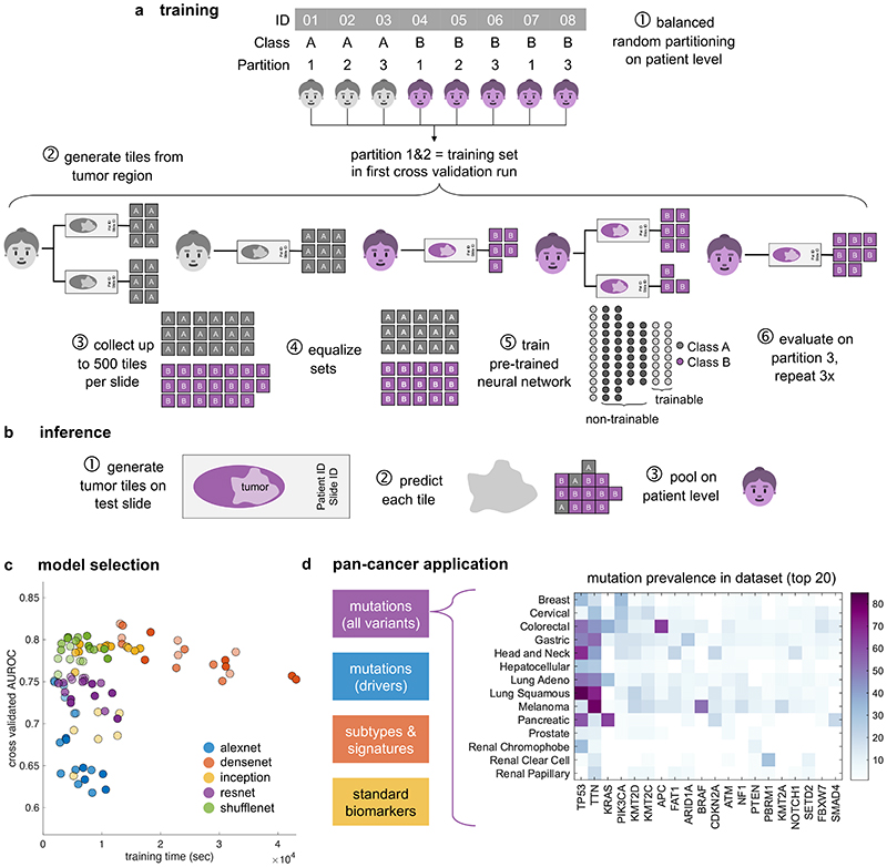
We hypothesized that deep learning can infer molecular alterations directly from routine histology images across multiple common solid tumor types. To test this, we developed, optimized and extensively validated a ‘one-stop-shop’ workflow to train and evaluate deep learning networks (Fig. 1a-b). To select an efficient network model and to optimize the deep learning hyperparameters, pre-diction of microsatellite instability (MSI) in colorectal cancer was used as a clinically relevant benchmark task¹⁰. In this benchmark, we sampled a large hyperparameter space with different commonly used deep learning models^10,11,14,16 which were modified specifically for this application. Unexpectedly, ‘shufflenet’¹⁷, a lightweight neural network architecture performed similarly to more complex networks including ‘densenet’¹⁸, ‘inception’¹⁹ and ‘resnet’²⁰ networks, which are used in many other studies²¹ (Fig. 1c). Shufflenet demonstrated high accuracy at a low training time (raw data in Suppl. Table 1, N=426 patients in the TCGA cohort). Shufflenet is optimized for mobile devices, making this deep neural network architecture attractive for decentralized point-of-care image analyses or direct imple-mentation in microscopes²². We externally validated the best shufflenet classifier by training on N=426 patients in the TCGA-CRC cohort¹⁰ and validating on N=379 patients with available MSI status in the DACHS cohort¹⁰, reaching an AUROC of 0.89 [0.88; 0.92]. This represents an improvement over the previous best performance of 0.84 in that dataset¹⁰ and supports the notion that shufflenet is an efficient and powerful neural network model which can infer clinically relevant molecular changes directly from histology images.

Fig. 1. Deep learning workflow for prediction of molecular features from histology images.

We describe a comprehensive method pipeline for prediction of molecular features directly from histological images. (a) Training of the deep learning system comprised six steps. Step 1: Patient cohorts were randomly split into three partitions for cross-validation of deep classifiers. Step 2: The tumor region on each whole slide image (WSI) was tessellated into tiles. Step 3: Up to 500 randomly chosen tiles were collected. Step 4: Tiles from patients in the training partitions were collected, classes were equalized by random undersampling. Step 5: All training tiles were used to train a deep neural network (pre-trained on a non-medical task). Step 6: Classification performance was evaluated on patients from the test partition. (b) For patient-level inference of molecular labels in patients not seen during training, three successive steps were used. Step 1: Tiles were generated from the tumor region on WSI. Step 2: A prediction was made for each tile. Step 3: Tile-level class predictions were pooled on a patient level. (c) Hyperparameters of the deep learning system were optimized in a benchmark task (prediction of microsatellite instability status [MSI] in colorectal cancer). The opacity of each point corresponds to the number of trainable layers. Shufflenet, a lightweight neural network architecture was selected as a highly efficient network model. (d) This workflow was subsequently applied for prediction of four types of molecular features across 14 cancer types. In particular, this included genetic mutations. The distribution of the 20 most common among all analyzed mutations is shown for each tumor type.

Pan-cancer prediction of genetic variants from histology

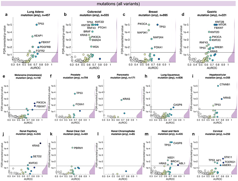
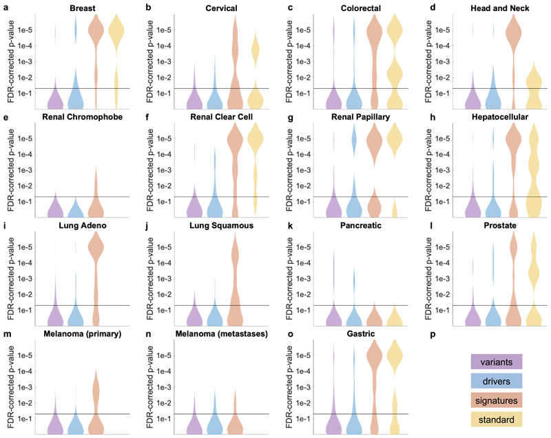
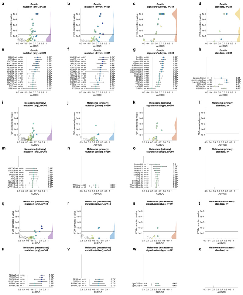
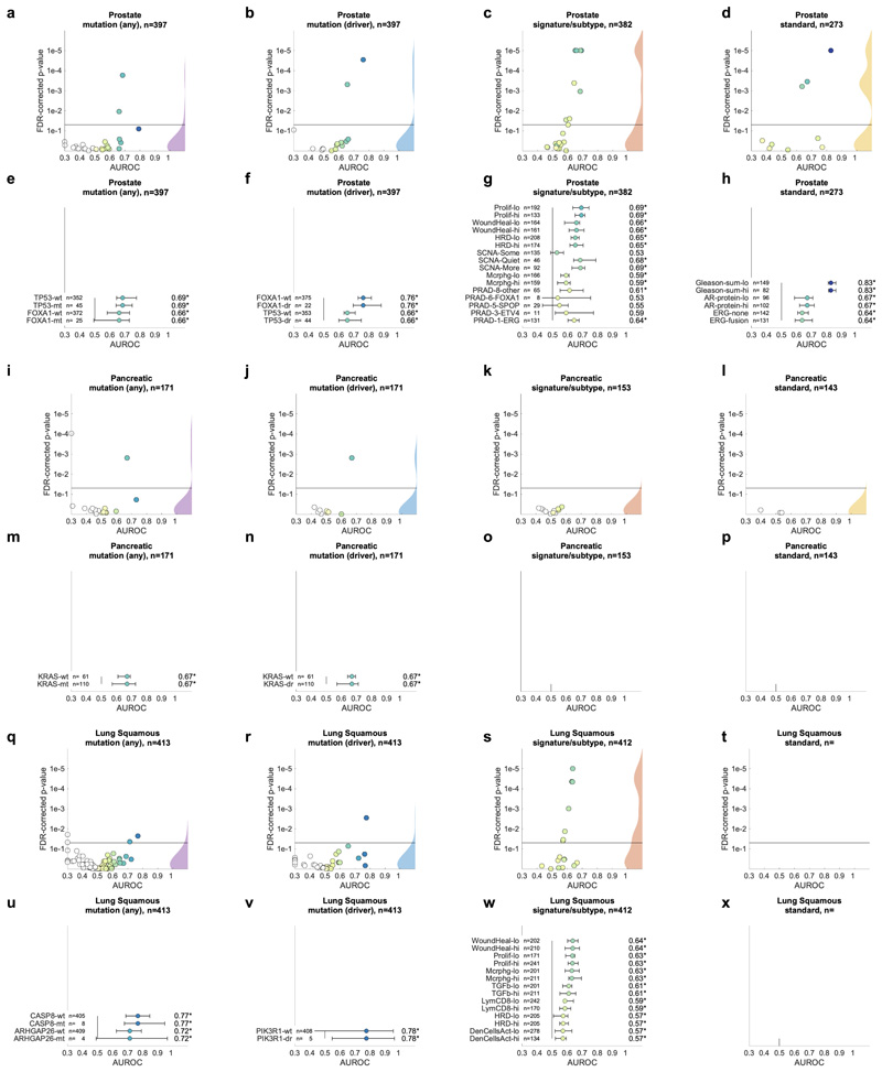
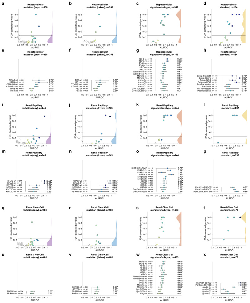
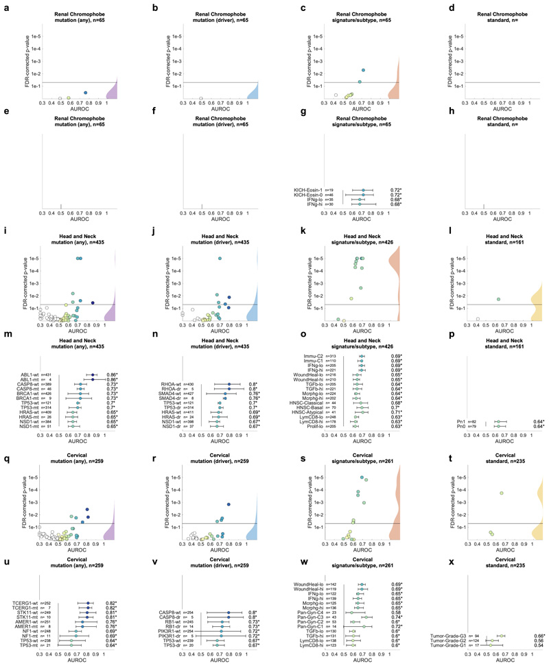
Having thus identified a deep neural network model and a set of suitable hyperparameters, we systematically applied this approach to hundreds of molecular alterations in 14 major tumor types, and trained and evaluated deep learning networks by three-fold cross-validation on each cohort. This yielded approximately 10⁴ independently trained deep neural networks which were systematically evaluated and compared across molecular features across cancer types. The full list of candidate mutations (Suppl. Table 1) included all point mutations targetable by FDA-approved drugs (Level 1 evidence on www.oncokb.org, the 20 most common mutations shown in Fig. 1d). First, we trained deep neural networks to detect any sequence variants in these target genes. We found that in 13 out of 14 tested tumor types, the mutation of one or more of such genes could be inferred from histology images alone, with statistical significance after correction for multiple testing (Fig. 2a-n, Extended Data Fig. 1). In particular, in major cancer types such as lung adenocarcinoma, colorectal cancer, breast cancer and gastric cancer, alterations of several genes of particular clinical and/or biological examples were detectable (Fig. 2a-d). Examples include mutations in TP53, which could be significantly detected in all four of these cancer types, as well as mutations of BRAF in colorectal cancer (TCGA-COAD and TCGA-READ²³, N=555, Fig. 2b), MTOR – a candidate for targeted treatment²⁴ – in gastric cancer (Fig. 2d) and FBXW7 mutation in lung adenocarcinoma (TCGA-LUAD²⁵, N=457, Fig. 2a) and gastric cancer (TCGA-STAD²⁶, N=321, Fig. 2d). Mutations of PIK3CA (which is directly targetable by a small molecule inhibitor²⁷) was significantly detectable in breast cancer (TCGA-BRCA²⁸, N=995, Fig. 2c) and gastric cancer (Fig. 2d). In addition, in breast cancer, mutations of MAP2K4 (which is a potential biomarker for response to MEK inhibitors²⁹) were significantly detectable (Fig. 2c). Among all tested tumor types, gastric cancer (Fig. 2d) and colorectal cancer (Fig. 2b) had the highest absolute number of detectable mutations. For all statistically significant features, the mean cross-validated area under the receiver operating curve (AUROC) for the top eight mutations ranged from 0.60 to 0.78 in lung adenocarcinoma (Extended Data Fig. 2a-h); from 0.65 to 0.76 in colorectal cancer (Extended Data Fig. 2i-p); from 0.62 to 0.78 in breast cancer (Extended Data Fig. 2q-x) and from 0.66 to 0.78 in gastric cancer (Extended Data Fig. 3a-h). Beyond these four tumor types, a range of notable mutations could be detected in other tumor types: While in melanoma (TCGA-SKCM³⁰) primary tumors, few mutations were detectable (Extended Data Fig. 3i-p), in melanoma metastases, mutations in FBXW7 and PIK3CA were sig-nificantly detectable (Fig. 2e, Extended Data Fig. 3q-x). In prostate cancer (TCGA-PRAD³¹, N=397 patients, Fig. 2f, Extended Data Fig. 4a-h), our method detected TP53 and FOXA1 mutations from histology, among others. In pancreatic adenocarcinoma (TCGA-PAAD³², N=171 patients, Fig. 2g, Extended Data Fig. 4i-p), identifying KRAS wild type patients is of high clinical relevance because these patients are potential candidates for targeted treatment and our method significantly identified KRAS genotype in pancreatic cancer. Lung squamous cell carcinoma is known for its difficulty in molecular diagnosis and few molecularly or genetically targeted treatment options even in clinical trials. Thus, it is plausible that in this cancer type, tumor histomorphology is not well correlated to mutations and correspondingly, few mutations were significantly detectable in this tumor type in our experiments (TCGA-LUSC³³, N=413, Fig. 2h, Extended Data Fig. 4q-x) In hepatocellular carcinoma (TCGA-LIHC³⁴, N=358 patients, Fig. 2i), the product of the β-catenin gene (CTNNB1) is a key driver gene with broad prognostic and predictive implications³⁵ and its mutational status was highly significantly detected from histology (Extended Data Fig. 5a-h). In papillary³⁶ (Fig. 2j, Extended Data Fig. 5i-p) and clear cell³⁷ renal cell carcinoma (Fig. 2k, Extended Data Fig. 5q-x), alterations in multiple genes including KRAS and PBRM were highly significantly detectable while in chromophobe³⁸ renal cell carcinoma (Fig. 2l, Extended Data Fig. 6a-h) no genetic variants were significantly detectable, possibly due to a low patient number in this cohort. In head and neck squamous cell carcinoma (TCGA-HNSC³⁹, N=435 patients), genotype of CASP8, which is linked to resistance to cell death⁴⁰, was significantly detected (Fig. 2m, Extended Data Fig. 6i-p). In cervical cancer (TCGA-CESC⁴¹, N=261 patients), mutations in TCERG1, STK11, AMER1, among others, were significantly detectable with high AUROC values (Fig. 2n, Extended Data Fig. 6x-q).

Fig. 2. Inference of genetic mutations from histological images.

A deep learning system was trained to predict mutational status (mutated or wild-type) of relevant genes in 14 cancer type and was evaluated by cross-validation. All mutations, including variants of unknown significance, were included in the ‘mutated’ class. For each gene, patient-level test set performance is shown as area under the receiver operating curve (AUROC) with two-sided t-test p-value for prediction scores corrected for multiple testing (false detection rate, FDR). The significance level of 0.05 is marked with a line and the distribution of p-values in each panel is shown as a density plot. P values smaller than 10⁻⁵ are set to 10⁻⁵. On the right-hand side of each panel, a kernel density estimate shows the distribution of all plotted data points. “n” denotes the number of patients with available genetic information and matched histology images in each tumor type. (a-d) In lung adenocarcinoma, colorectal cancer, breast cancer and gastric cancer, a number of relevant genes were significantly predictable from histology alone, including key oncogenic drivers such as TP53, BRAF and MTOR. (e-n) In all other tested tumor types, mutational status was predictable for some genes, with notable examples including KRAS in pancreatic cancer, CTNNB1 in hepatocellular carcinoma and TP53 and CASP8 in head and neck cancer.

Pan-cancer prediction of oncogenic drivers from histology

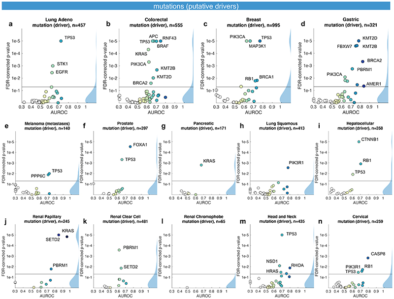
Not all genetic variants are causative of malignant processes. Therefore, we repeated the screening experiment, limiting mutations to confirmed or putative oncogenic drivers (Fig. 3a-n). With this criterion, the absolute number of patients affected by a particular mutation was lower and thus, fewer genes met the threshold of at least four positive cases in a given tumor type. On the other hand, we hypothesized that oncogenic driver genes could leave a stronger pattern in histological morphology due to their higher biological relevance. Genetic variants in classical oncogenes such as TP53 and KRAS are almost always oncogenic drivers and correspondingly, mutations of these genes reached similar prediction accuracy valued in the “drivers only” experiment when compared to the “all variants” approach (Fig. 3a-n). For mutations in other genes, prediction accuracy increased when limited to oncogenic drivers: a notable example was EGFR in lung adenocarcinoma (Fig. 3a). In summary, these data show that deep learning can detect targetable and potentially targetable point mutations in a wide range of genes directly from histology across multiple prevalent tumor types.

Fig. 3. Inference of putative oncogenic drivers from histological images.

A deep learning system was trained to predict oncogenic driver genes from histology. Only putative and confirmed drivers were included and variants of unknown significance were pooled with the “wild type” class. On the right-hand side of each panel, a kernel density estimate shows the distribution of all plotted data points. “n” denotes the number of patients with available genetic information and matched histology images in each tumor type. The layout of this figure corresponds to Fig. 2. (a-n) This process uncovered significant predictability of multiple oncogenic drivers, including EGFR, BRAF and TP53.

Inference of molecular subtypes and gene expression signatures

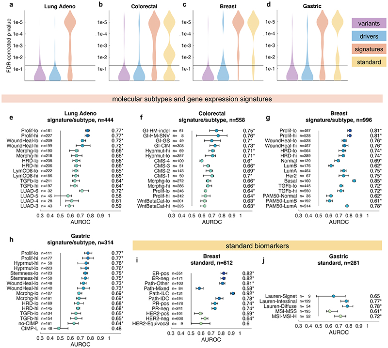
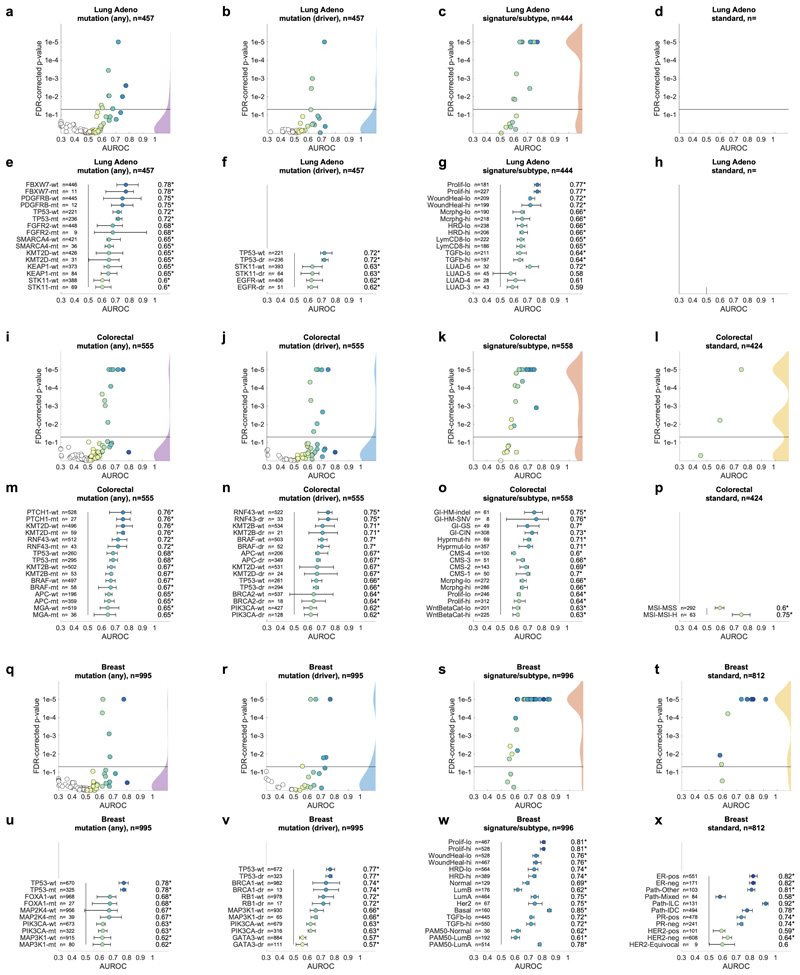
In the next step, we asked if established molecular subtypes and gene expression signatures of cancer and immune cells could be detected by deep learning. Compared to single-gene mutations, these changes occur at a higher functional level and we hypothesized that their morphological impact could be larger than that of single mutations. To address this hypothesis, we chose features with known biological and potential clinical significance. A major group of such features are immune-related gene expression signatures⁴² of CD8-positive lymphocytes, macrophages, cell proliferation, interferon-gamma (IFNg) signaling and transforming growth factor-beta (TGFb) signaling (full list available in Suppl. Table 1). These biological processes are involved in response to cancer treatment, including immunotherapy. Detecting their morphological correlates in histology images could facilitate the development of more nuanced treatment strategies. Indeed, across all investigated tumor types, we saw that these high-level biological features were much better predictable than genetic variants or driver mutations (Fig. 4a-d and Extended Data Fig. 1) Again, AUROC values for significantly (p<0.05 after FDR correction) predictable features were highest in lung adenocarcinoma (Fig. 4e), colorectal cancer (Fig. 4f), breast cancer (Fig. 4g) and gastric cancer (Fig. 4h). In lung adenocarcinoma, signatures of proliferation, macrophage infiltration and T-lymphocyte infiltration were significantly detectable from images with high AUROCs (Fig. 4e). Similarly, significant AUROCs for these biomarkers were achieved in colorectal cancer (Fig. 4f) breast cancer (Fig. 4g) and gastric cancer (Fig. 4h). In gastric cancer, we additionally found that a signature of stem cell properties (stemness) was highly detectable directly from histology images (Fig. 4h). Recent studies have clustered tumors into comprehensive ‘molecular subtypes’⁴². We found that our method could detect TCGA molecular subtypes⁴² with up to AUROC 0.74 in lung adenocarcinoma (Fig. 4e), pan-gastrointestinal subtypes⁴³ with up to AUROC 0.76 in colorectal cancer (Fig. 4f) and PAM50 subtypes with up to AUROC 0.78 in breast cancer (Fig. 4g), among other molecular subtypes. These findings could open up new options for clinical trials of cancer: While accumulating evidence shows that such molecular clusters of tumors reflect biologically distinct groups and are correlated to clinical outcome, deep molecular classification of these tumors is usually not available in clinical routine or clinical trials. Detecting these subtypes merely from histology would allow for these subtypes to be analyzed in clinical trials directly from broadly available routine material, potentially helping to identify new biomarkers for treatment response or to guide specific molecular testing.

Fig. 4. Inference of molecular subtypes, gene expression signatures and standard biomarkers directly from histology.

In addition to prediction of singlegene mutations, the capability of deep learning to infer high-level molecular features was systematically assessed. (a-d) In lung, colorectal, breast and gastric cancer, gene expression signatures (such as TCGA molecular subtype in any tumor type) and standard of care features (such as hormone receptor status in breast cancer) were highly predictable from histology alone, as shown by the distribution of two-sided t-test false-detection rate (FDR)-corrected p-values as visualized by a kernel density estimate. Individual data points are shown in Extended Data Figures 2-6. (e-h) Gene expression signatures for Proliferation (Prolif), Wound Healing (WoundHeal), Macrophage infiltration (Mcrphg), Homologous Repair Deficiency (HRD), CD8-positive Lymphocyte (LymCD8), TCGA molecular subtypes (LUAD 1-6), pan-gastrointestinal (GI) molecular subtypes, consensus molecular subtypes (CMS), PAM50 subtypes and other key molecular features were highly predictable across multiple tumor types. Error bars show patient-level AUROC with bootstrapped confidence intervals, the marker denotes the mean, * denotes two-sided t-test FDR-corrected p-value< 0.05. „n“ refers to the number of patients. (i-j) Standard of care biomarkers including estrogen and progesterone receptor (ER and PR) status in breast cancer, pathologic subtype and microsatellite instability (MSI) were highly predictable from routine histology alone by deep learning.

Prediction of standard histological biomarkers with deep learning

To comprehensively evaluate the potential clinical use of our deep learning pipeline, we investigated classification accuracy for standard histopathological biomarkers. We found that deep learning could highly significantly predict most of these biomarkers for breast cancer (Fig. 4c and i), gastric cancer (Fig. 4d and j) and other tumor types. In particular, status of hormone receptors was predictable from routine histology in breast cancer, with an AUROC of 0.82 for estrogen receptor and 0.74 for progesterone receptor (Fig. 4i). Together, these results demonstrate that deep-learning-based inference of genetic alterations, high-level molecular alterations and established biomarkers from routine diagnostic histology slides is feasible.

Evaluation of alternative approaches

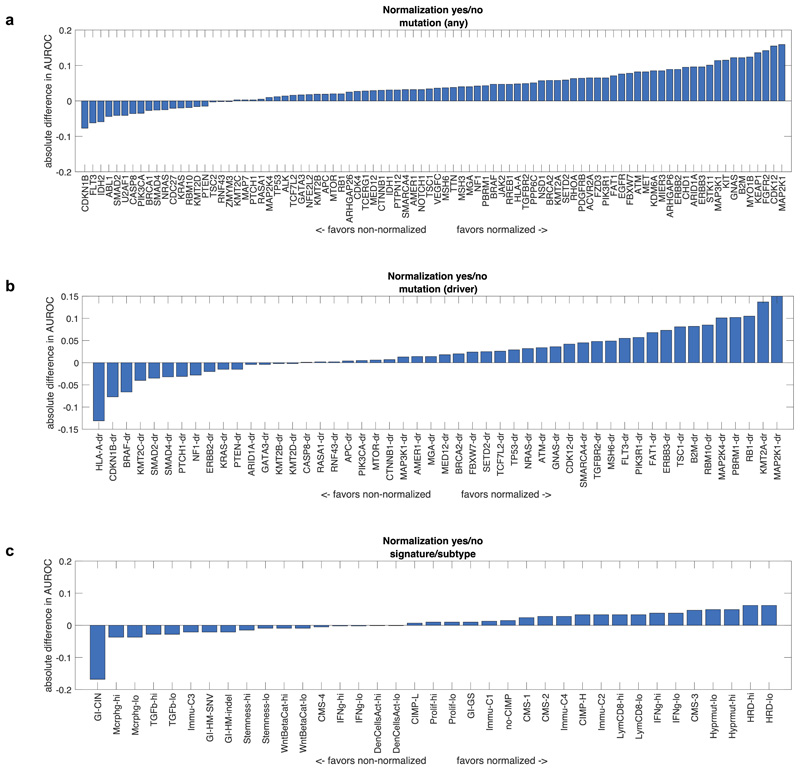
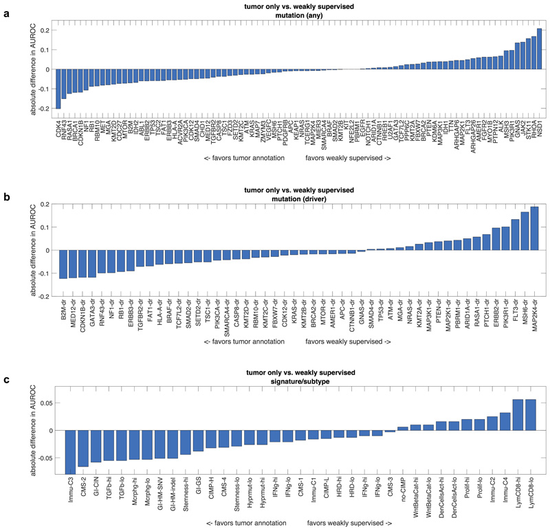
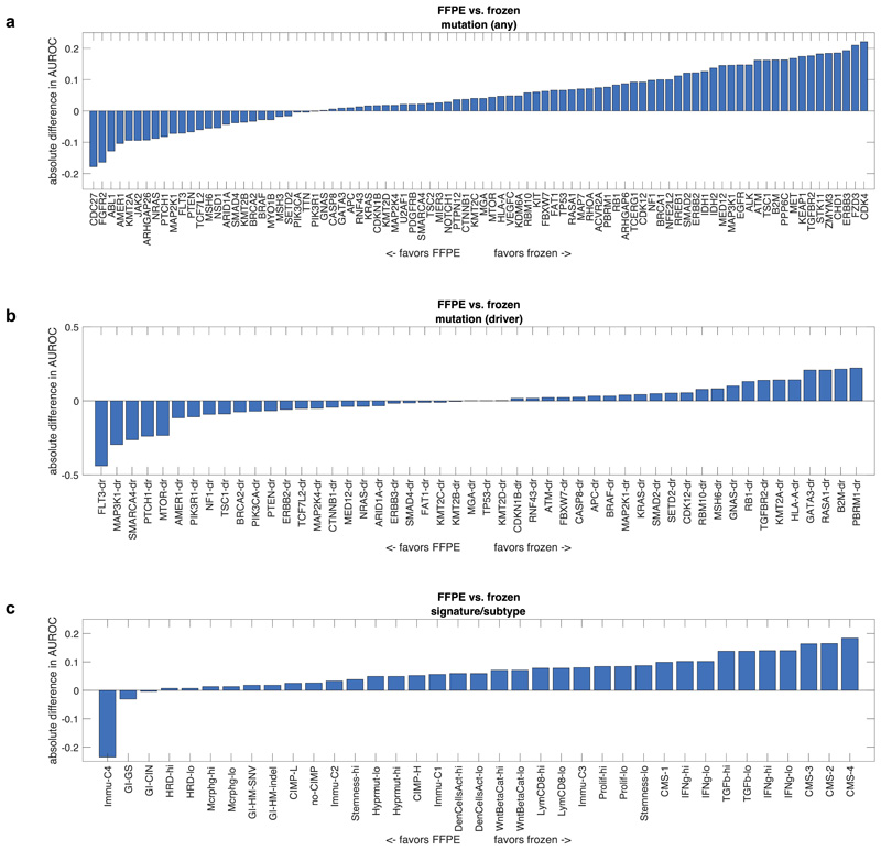
Deep learning-based inference of molecular features from histology is a relatively novel field of research and it can be anticipated that technical improvements can further improve prediction performance. We quantified the effect of alternative technical approaches in the colorectal cancer cohort (TCGA-COAD/READ). First, we investigated the role of color normalization of tiles. In a head-to-head comparison to the baseline approach, we found a tendency of Macenko’s⁴⁴ color normalization to improve classifier performance for mutation prediction but not for prediction of subtypes or gene expression signatures (Extended Data Fig. 7a-c). Second, we investigated a weakly supervised approach to our baseline of expert-annotated tumor regions and found that the weakly supervised approach was only slightly inferior to manual annotation (Extended Data Fig. 8a-c). Third, we analyzed prediction performance on frozen slides compared to diagnostic slides. While frozen slides are not generally available in a clinical setting, the TCGA database provides an opportunity to perform such a direct comparison. In a weakly supervised experiment, we found that prediction power for driver genes was on par, but prediction power for genetic variants and high-level subtypes/signatures was better in frozen slides than in diagnostic slides (Extended Data Fig. 9a-c). These data provide quantitative guidance for future large-scale validation studies.

External validation of the classification results

Deep learning approaches to a single dataset are prone to overfit and should be validated in external populations before clinical deployment. For external validation of our method, we used routine H&E slides of N=408 colorectal cancer patients from the DACHS study for which BRAF mutational status and CpG-island methylator phenotype (CIMP) was available. We trained deep learning classifiers for BRAF and CIMP on TCGA colorectal cancer samples and evaluated the patient-level accuracy on DACHS. Both features were statistically significantly detectable from DACHS H&E images alone: For BRAF mutants, AUROC was 0.77 (0.64 – 0.82, p<10⁻⁵) and for CIMP-high, AUROC was 0.66 [0.56– 0.72, p<10⁻⁵). These data show that deep-learning-based prediction of clinically relevant genetic features can generalize to external patient populations.

Discussion

Image-based genetic testing as a clinical and research tool

Our results demonstrate the feasibility of pan-cancer deep-learning-based inference of a broad range of molecular and genetic features directly from histological images. We show that a unified workflow yields reliably high performance across multiple clinically relevant scenarios without the need to tune technical parameters to a specific molecular target. Our systematic screening approach identifies candidate genetic variants, driver genes, gene expression signatures and standard of care features that can be significantly inferred from histology images, opening up perspectives for large-scale validation of these candidate markers. As a large-scale, systematic screening study, this work identifies a number of mutations which are significantly linked to a detectable phenotype in histological images, including those in key oncogenic pathways including the products of TP53, FBXW7, KRAS, BRAF and CTNNB1. In addition to individually mutated genes, our data show that higher-level gene expression clusters or signatures can be inferred from histological images. Many of these clusters represent groups of patients with distinct and well-described cancer biology such as consensus molecular subtype (CMS) in colorectal cancer. By linking these molecularly defined groups to specific histological image features, our method constitutes a tool to decipher downstream biological effects of molecular alterations in solid tumors. In an external validation cohort, we show that the models trained on images from the TCGA archive generalize to external patients, demonstrating the potential of applying these methods to routine material from real-world clinical cohorts. Of note, additional retrospective and prospective validation and regulatory approval is needed for histology-based deep learning methods to be implemented in clinical workflows. An example for clinical implementation would be the use as pre-screening tools to enrich patient populations for specific molecular testing. While it is expected that the first applications of deep learning technology in routine workflows will relate to the automatic identification of tumor tissues for the selection of specimens or regions of interest, our method could be easily added to such digital pathology workflows, providing a strong additional incentive for digitization of histopathology.

Limitations

Currently, limitations of our method are the low AUROC values for some molecular features (Fig. 2 and Fig. 3). A strategy to increase the diagnostic performance would be re-training on larger patient cohorts. Re-training can be expected to boost performance because previous studies have shown that performance of deep learning systems in histopathology scales with the number of patients in the training cohort.¹⁶ In addition, the performance of deep learning systems could potentially be improved by technical modifications. Our systematic evaluation of alternative technical approaches provides a guidance for this on multiple levels: First, regarding the choice of neural network models, our results demonstrate that lightweight neural network models perform on par with more complex models, facilitating further evaluation of these methods on decentralized hardware, including desktop or ultimately mobile hardware. While this finding is based on a clinically relevant benchmark task and generalizes to an external population, we cannot exclude that other network models perform better in other histology applications. Second, regarding the type of input image data, other studies in digital pathology have used frozen histology sections¹¹. In contrast, our baseline workflow was based on FFPE tissue slides (labeled as ‘diagnostic slides’ in the TCGA archive) due to their clinical relevance. In clinical settings, frozen specimens constitute only a small fraction of pathology samples and therefore, establishing methods on FFPE material is paramount for large-scale clinical validation. Our head-to head comparison shows that molecular inference generally works better on frozen slides, which is a limitation of the FFPE-based method. Further studies are needed to determine the reasons for this observation. Lastly, our baseline method relied on expert annotations of tumor tissue, constraining deep learning models to learn from invasive tumor tissue only. The rationale behind this design was that despite advances in computer vision, expert annotation of tumor tissue remains the gold standard in histopathology studies. Yet, in a head-to-head comparison, a weakly supervised approach without any manual annotation did not markedly reduce performance, demonstrating feasibility of even simpler data preprocessing pipelines. Ultimately, fully automatic workflows can be expected to be superior to manual workflows in terms of scalability and reproducibility. We publicly release all source codes of our method, enabling further optimization and validation on a larger scale.

Deciphering genotype-phenotype links

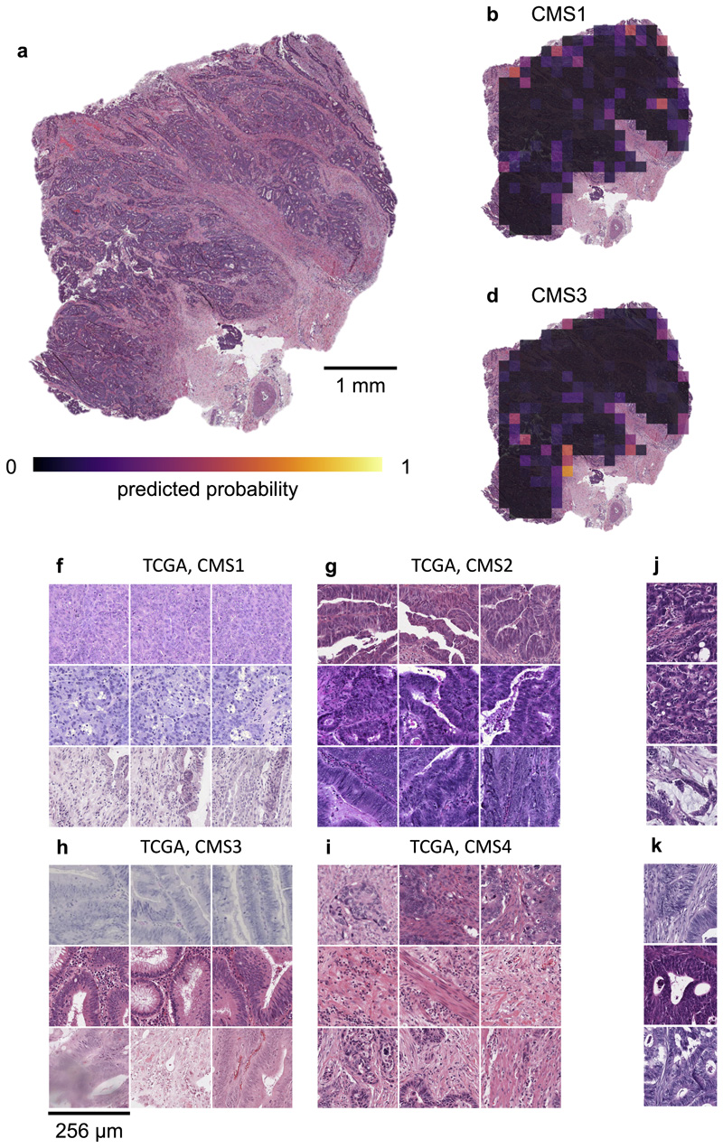
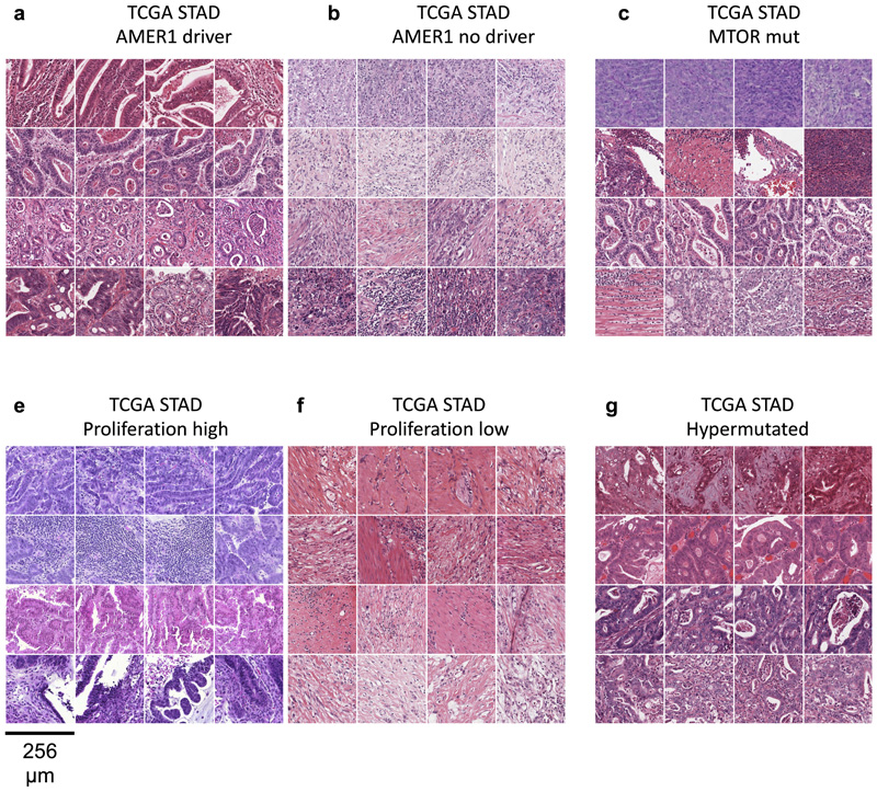
Beyond being a potentially useful tool for clinical applications, deep learning-based inference of molecular features from morphology could shed light on more fundamental properties of cancer biology. Our study systematically screens hundreds of molecular alterations and identifies candidates that are linked to detectable patterns in histology images. These patterns can be visualized through prediction maps (Fig. 5a-e). Such “spatialization” of genetic predictions is a key aspect lacking in conventional bulk genetic tests of tumor and could be useful to trace back molecular alterations to specific spatial regions. An alternative approach to understanding deep-learning-based predictions is through visualization of highly ranked image tiles (Fig. 5f-k). This approach can serve as a plausibility control and may help to discover new morphological features. Indeed, highly ranked tiles of CMS classes in colorectal cancer showed poorly differentiated tumor in CMS1 tiles (Fig. 5f), well-differentiated glands for CMS2-3 (Fig. 5g-h) and highly stromal tiles for CMS4 (Fig. 5i). These patterns correspond to known biological processes underlying CMS subclasses, corroborating the assumption that our deep learning system detects biologically meaningful features. Similarly, visualizing histomorphology in the highest predicted tiles in BRAF mutant patients in the validation cohort (Fig. 5j-k) demonstrated poorly differentiated areas and mucinous areas as recurring features in BRAF mutant image tiles, which is consistent with previous studies.⁴⁵ Visualizing highly predicted tiles in gastric cancer (Fig. 6 a-h) highlighted highly cellular areas as correlates of a “Proliferation” gene expression signature, but at the same time identified patterns for mutations (e.g. in AMER1 and MTOR) which could help to form new hypotheses on how these specific mutations influence cancer cell behavior and morphology. Interestingly, the prediction performance markedly varied between the 14 different types of cancer (Fig. 2, Extended Data Fig. 1). Variations in sample size between the cohorts could explain some of these differences, but additional biological effects could contribute to this. One hypothesis is that tumor types with few clinically targetable mutations (e.g. lung squamous cell cancer and pancreatic cancer) also display few detectable mutations. Further studies are warranted to investigate this.

Fig. 5. Explainability of deep learning-based analysis of histological images.

Deep learning-based predictions were visualized through genotype maps and comparison of highly ranked image tiles. (a-e) Prediction maps for consensus molecular subtype (CMS) in colorectal cancer show spatially resolved prediction scores, unveiling intratumor heterogeneity of predicted genotype. As a generic tool, this visualization approach allows to identify spatial regions associated with a molecular feature. In this patient, the correct prediction of CMS4 correctly show that deep learning robustly predicts CMS from histology alone while highlighting potential intratumor heterogeneity (f-i) For each of the CMS classes, the most highly scored test set tiles are shown, enabling correlation of deep learning-predictions with histopathological features at high resolution. In this case, highly predicted CMS1 tiles contain numerous tumorinfiltrating lymphocytes while predicted CMS4 tiles contain abundant stroma, consistent with previous studies. (j-k) Highly scored tiles in the external test cohort DACHS for prediction of BRAF mutant and wild type (l-m) and CpG-island methylator phenotype (CIMP) high or non-CIMP.

Fig. 6. Highest scoring image tiles for molecular features in gastric cancer.

(a-b) Highest scoring tiles in highest scoring patients corresponding to AMER1 mutational status in the TCGA-STAD data set. (c-d) Tiles corresponding to MTOR mutational status. (e-f) Tiles corresponding to high or low values of a proliferation signature. (a-b) Tiles corresponding to hypermutated samples.

Conclusion

Together, our results demonstrate that molecular changes in solid tumors can be inferred from routine histology alone with deep learning. This could be a useful tool to objectively elucidate genotype-phenotype relationships in cancer and ultimately, could be used as a low-cost biomarker in clinical trials and routine clinical workflows.

Methods

Patient cohorts and ethics statement

All experiments were conducted in accordance with the Declaration of Helsinki and the International Ethical Guidelines for Biomedical Research Involving Human Subjects. Anonymized scanned whole slide images were retrieved from The Cancer Genome Atlas (TCGA) project through the Genomics Data Commons Portal (https://portal.gdc.cancer.gov/). We applied our method to 14 of the most common solid tumor types: breast (BRCA)²⁸, cervical (CESC)⁴¹, colorectal (COAD and READ)²³, gastric (STAD)²⁶, head and neck (HNSC)³⁹, hepatocellular (LIHC)³⁴, lung adeno (LUAD)²⁵, lung squamous (LUSC)³³, melanoma (SKCM)³⁰, pancreatic (PAAD)³², prostate (PRAD)³¹, renal cell chromophobe (KICH)³⁸, renal cell clear cell (KIRC)³⁷ and renal cell papillary cancer (KIRP)³⁶. Melanoma (SKCM) tissue slides in the TCGA database comprised primary tumor samples as well as metastasis tissue. These groups were analyzed separately. For external validation, we acquired colorectal cancer tissue samples from the DACHS study^46,47, which were retrieved from the tissue bank of the National Center for Tumor Diseases (NCT, Heidelberg, Germany) as described before.¹⁰ Ethics oversight of the TCGA study is described at https://www.cancer.gov/about-nci/organization/ccg/research/structural-genomics/tcga/history/policies and ethical approval of the DACHS study was given by the ethics committee of the Medical Faculty of the University of Heidelberg. Informed consent was obtained by all participants in the TCGA and DACHS studies.

Molecular labels

The aim of this study was to predict clinically relevant features, including genetic alterations, directly from routine histology slides. We systematically applied this screening approach to four groups of molecular alterations: First, we used single-gene mutations, considering any genetic variant. We used the most commonly mutated genes in the respective tumor types (derived from the “cbioportal” database^48,49 at http://cbioportal.org) and clinically targetable genes (level one genes from OncoKB at http://www.oncokb.org, Pan Cancer Atlas Project⁵⁰). We required each mutation to affect at least four patients in a given cohort. Second, we repeated the analysis on putative and confirmed oncogenic driver mutations only, as defined in OncoKB. Third, we aimed to predict gene expression subtypes, relevant gene expression signatures and immune-cell gene expression signatures derived from systematic studies^42,43,51. Fourth, we used “standard of care” features derived from the TCGA database (data at http://portal.gdc.cancer.gov), including hormone receptor status in breast cancer. All labels (genetic variants, driver mutations, signatures and standard features) are listed in Suppl. Table 1. For each individual target label in each tumor type and each cross-validation run, we re-trained a single deep neural network, using identical hyperparameters. Features with continuous values were binarized at the mean.

Image preprocessing

Scanned whole slide images of diagnostic tissue slides (formalin-fixed paraffin-embedded tissue) stained with hematoxylin and eosin were acquired in SVS format. All images were downsampled to 20x magnification, corresponding to 0.5 μm/pixel (px). Each whole slide image was manually reviewed and the tumor area with was annotated under direct supervision of a specialty pathologist. During annotation, all observers were blinded with regard to any molecular or clinical feature. Only those images containing at least 1 mm² contiguous tumor tissue were used for downstream analysis. 6% of whole slide images, corresponding to 5% of patients were excluded due to technical artifacts or lack of tumor (Suppl. Table 2). Tumor tissue on all other slides was tessellated into square tiles of 512x512 px edge length, corresponding to 256x256 μm at a resolution of 0.5 μm/px. Tiles with more than 50% background were discarded; background pixels were defined by brightness over 0.86 (220/255). For the benchmark task (identification of an optimal neural network model), these images were resized to 224x224 px (at 1.14 μm/ px) to be consistent with a previous study¹⁰. All steps in the data preprocessing pipeline (including preprocessing of images and preprocessing of metadata) are documented in detail in our in-house manual for data preparation, which is publicly available at https://dx.doi.org/10.5281/zenodo.3694994. All methods for whole slide image processing, including tessellation of images and visualization of spatial activation maps, were implemented in QuPath⁵² v0.1.2 in Groovy (http://qupath.github.io).

Patient-level cross-validation

Aiming to develop a one-stop-shop method for systematic discovery of genotype-phenotype links in multiple cancer types, we developed a reusable pipeline of data processing steps. One or more whole slide images (WSI) per patient were collected tumor regions in these images were tessellated into tiles. All tiles inherited the molecular label of their parent patient. Before training, the patient cohort was randomly split in three partitions, keeping the target labels balanced between partitions. Neural networks were trained on two partitions each and subsequently evaluated on the third partition. Thus, no tiles from a given patient were ever part of a training set and a test set for the same classifier. Before training, tile libraries were randomly undersampled in such a way that the number of tiles per label was identical for each label (Fig. 1a).

Neural network training, model selection and hyperparameter optimization

Deep neural networks were trained on image tiles with the aim of predicting molecular labels. All neural networks were pre-trained on the ImageNet database as described previously¹⁰ and were specifically modified for the classification task at hand by replacing the three top layers with a 1000-neuron fully connected layer, a softmax layer and a classification layer. For training, we used on-the-fly data augmentation (random horizontal and vertical reflection) to achieve rotational invariance of the classifiers. Hyperparameter selection was performed for five commonly used deep neural networks: resnet18, alexnet, inceptionv3, densenet201 and shufflenet. The sampled hyperparameter space was as follows: learning rate 5e-5 and 1e-4, maximum number of tiles per whole slide image: 250, 500 and 750, number of trainable layers: 10, 20 and 30. We trained for four epochs with a mini batch size of 512, similar to previous experiments.¹⁰ As a benchmark task, we used MSI detection in colorectal cancer as described before.¹⁰

Inference of molecular status

During inference, a categorical prediction was made for each tile by the neural network (Fig. 1b). The percentage of positive predicted tiles for each class was regarded as a “probability score” for each patient. This score was used as the free variable for a receiver operating characteristic (ROC) analysis with area under the ROC curve (AUROC) being the primary endpoint for each target feature.

Alternative approaches

In our baseline approach, image tiles from manually annotated tumor regions on formalin-fixed paraffin-embedded (FFPE) slides (diagnostic slides) were used. This approach was compared to several alternative approaches as shown in Extended Data Fig. 7, 8 and 9. The first alternative approach used color normalization of image tiles with the Macenko method⁴⁴ to mitigate differences in staining intensity and hue (Extended Data Fig. 7). Some previous studies have used color normalization for deep learning¹⁰, while other studies have shown that color normalization can bias histology image classification.⁵³ The second alternative approach we investigated was to use tiles from the whole slide, as opposed to the tumor region only. In this “weakly supervised” approach, many tiles without invasive cancer tissue were present in the training and inference sets (Extended Data Fig. 8). The third alternative approach was to use frozen slides as opposed to FFPE slides in a weakly supervised way (Extended Data Fig. 9).

Statistics and reproducibility

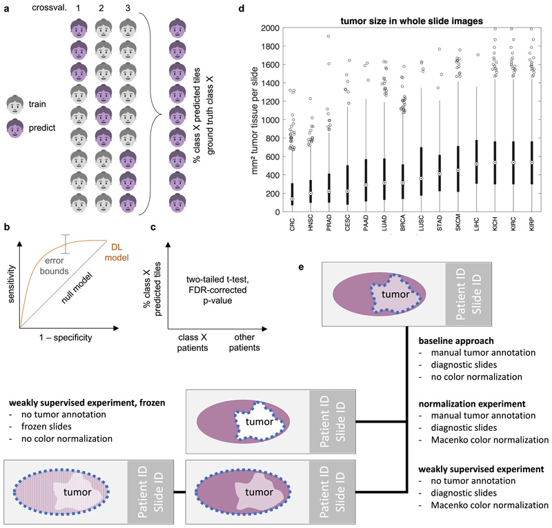
AUROC values are reported as mean with a confidence interval representing lower and upper range of a 10x bootstrapped experiment. To quantify if predictions for different classes of patients were statistically significant, the probability scores for patients in a given class were compared to probability scores of all other patients. Statistical significance of these differences was assessed with a two-sided t-test with a pre-defined significance level of 0.05. To compensate for the large number of tested hypotheses in this study, we performed “false detection rate” (FDR) correction for p-values with the Benjamini-Hochberg method on all p-values across all cancer types. All p-values smaller than 10⁻⁵ after FDR-correction are reported as 10⁻⁵. Statistical methods are further described in Extended Data Fig. 10a-c. The number of tiles generated per whole slide image is shown in Extended Data Fig. 10d. No statistical method was used to predetermine sample size. The Investigators were blinded to molecular status of samples during manual annotation, image processing procedures and outcome assessment. Source codes are publicly available, allowing to replicate our findings. The investigators re-ran the computer codes three times, receiving identical results. Further information on research design is available in the Nature Research Reporting Summary linked to this article.

Implementation and hardware

Training and inference were performed on our local computing cluster on 10 Nvidia RTX graphics processing units (GPUs), each with 24 GB of GPU RAM. Cumulative computing time for all experiments within this study was approximately 12,000 GPU-hours. All deep learning algorithms were implemented in Matlab R2019a (Mathworks, Natick, MA, USA).

External validation

To investigate if complex deep learning biomarkers generalize to external patient cohorts, we trained deep learning classifiers on all TCGA samples of a given tumor type and externally validated the predictions in patient cohorts from our respective institutions. External validation was performed for BRAF mutation status and CpG island methylator phenotype (CIMP) in colorectal cancer in N=408 patients, a subset of the multicenter DACHS study which was previously collected and described.¹⁰ BRAF and CIMP were chosen as validation markers because of their biological relevance and availability of robust measurements of these markers in the DACHS cohort.

Feature visualization

To visualize the deep learning predictions and make them understandable to human observers, we used two approached: First, we rendered the tile-level soft predictions for each class as activation maps, visualizing prediction scores as a heatmap overlay on the original histology image. Second, we identified the highest-predicted tiles of the highest-predicted true positive patients for each class, allowing observers to identify histological patterns that are correlated with a molecular feature. These approaches were designed to allow human observers to identify which morphological features deep learning classifiers were most sensitive to.

Extended Data

Extended Data Fig. 1.

Extended Data Fig. 2.

Extended Data Fig. 3.

Extended Data Fig. 4.

Extended Data Fig. 5.

Extended Data Fig. 6.

Extended Data Fig. 7.

Extended Data Fig. 8.

Extended Data Fig. 9.

Extended Data Fig. 10.

Data availability

All data, including histological images and information about age and sex of the participants from the TCGA database are available at https://portal.gdc.cancer.gov/. Genetic data for patients in the TCGA cohorts are available at https://portal.gdc.cancer.gov/ and https://cbioportal.org. Raw data for the DACHS cohort are stored and administered by the DACHS consortium (more information on http://dachs.dkfz.org/dachs/). The corresponding authors of this study are not involved in data sharing decisions of the DACHS consortium. Source data for Figs. 1–4 and Extended Data Figs. 1-10 have been provided as Source Data File 1–14. All other data supporting the findings of this study are available from the corresponding author on reasonable request.

Code availability

All source codes are available under an open source license at https://github.com/jnkather/DeepHistology/releases/tag/v0.2.

Bibliography

- 1.Cheng ML, Berger MF, Hyman DM, Solit DB. Clinical tumour sequencing for precision oncology: time for a universal strategy. Nature Reviews Cancer. 2018;18:527–528. doi: 10.1038/s41568-018-0043-2. [DOI] [PMC free article] [PubMed] [Google Scholar]
- 2.Rusch M, et al. Clinical cancer genomic profiling by three-platform sequencing of whole genome, whole exome and transcriptome. Nature Communications. 2018;9 doi: 10.1038/s41467-018-06485-7. 3962. [DOI] [PMC free article] [PubMed] [Google Scholar]
- 3.Kather JN, Halama N, Jaeger D. Genomics and emerging biomarkers for immunotherapy of colorectal cancer. Seminars in Cancer Biology. 2018;52:189–197. doi: 10.1016/j.semcancer.2018.02.010. [DOI] [PubMed] [Google Scholar]
- 4.Guinney J, et al. The consensus molecular subtypes of colorectal cancer. Nature Medicine. 2015;21 doi: 10.1038/nm.3967. 1350. [DOI] [PMC free article] [PubMed] [Google Scholar]
- 5.Fontana E, Eason K, Cervantes A, Salazar R, Sadanandam A. Context matters-consensus molecular subtypes of colorectal cancer as biomarkers for clinical trials. Ann Oncol. 2019;30:520–527. doi: 10.1093/annonc/mdz052. [DOI] [PMC free article] [PubMed] [Google Scholar]
- 6.Shia J, et al. Morphological characterization of colorectal cancers in The Cancer Genome Atlas reveals distinct morphology-molecular associations: clinical and biological implications. Modern pathology : an official journal of the United States and Canadian Academy of Pathology, Inc. 2017;30:599–609. doi: 10.1038/modpathol.2016.198. [DOI] [PMC free article] [PubMed] [Google Scholar]
- 7.Greenson JK, et al. Pathologic predictors of microsatellite instability in colorectal cancer. The American journal of surgical pathology. 2009;33:126–133. doi: 10.1097/PAS.0b013e31817ec2b1. [DOI] [PMC free article] [PubMed] [Google Scholar]
- 8.Greenson JK, et al. Pathologic predictors of microsatellite instability in colorectal cancer. Am J Surg Pathol. 2009;33:126–133. doi: 10.1097/PAS.0b013e31817ec2b1. [DOI] [PMC free article] [PubMed] [Google Scholar]
- 9.Le DT, et al. PD-1 Blockade in Tumors with Mismatch-Repair Deficiency. New England Journal of Medicine. 2015;372:2509–2520. doi: 10.1056/NEJMoa1500596. [DOI] [PMC free article] [PubMed] [Google Scholar]
- 10.Kather JN, et al. Deep learning can predict microsatellite instability directly from histology in gastrointestinal cancer. Nature Medicine. 2019 doi: 10.1038/s41591-019-0462-y. [DOI] [PMC free article] [PubMed] [Google Scholar]
- 11.Coudray N, et al. Classification and mutation prediction from non-small cell lung cancer histopathology images using deep learning. Nature Medicine. 2018;24:1559–1567. doi: 10.1038/s41591-018-0177-5. [DOI] [PMC free article] [PubMed] [Google Scholar]
- 12.Sha L, et al. Multi-Field-of-View Deep Learning Model Predicts Nonsmall Cell Lung Cancer Programmed Death-Ligand 1 Status from Whole-Slide Hematoxylin and Eosin Images. J Pathol Inform. 2019;10:24. doi: 10.4103/jpi.jpi_24_19. [DOI] [PMC free article] [PubMed] [Google Scholar]
- 13.Schaumberg AJ, Rubin MA, Fuchs TJ. H&E-stained Whole Slide Image Deep Learning Predicts SPOP Mutation State in Prostate Cancer. bioRxiv. 2018 064279. [Google Scholar]
- 14.Kather JN, et al. Deep learning detects virus presence in cancer histology. bioRxiv. 2019 690206. [Google Scholar]
- 15.Zhang H, et al. Predicting Tumor Mutational Burden from Liver Cancer Pathological Images Using Convolutional Neural Network. 2019 IEEE International Conference on Bioinformatics and Biomedicine (BIBM); 2019. pp. 920–925. [Google Scholar]
- 16.Campanella G, et al. Clinical-grade computational pathology using weakly supervised deep learning on whole slide images. Nature Medicine. 2019 doi: 10.1038/s41591-019-0508-1. [DOI] [PMC free article] [PubMed] [Google Scholar]
- 17.Zhang X, Zhou X, Lin M, Sun J. Shufflenet: An extremely efficient convolutional neural network for mobile devices. Proceedings of the IEEE Conference on Computer Vision and Pattern Recognition; 2018. pp. 6848–6856. [Google Scholar]
- 18.Huang G, Liu Z, Van Der Maaten L, Weinberger KQ. Densely connected convolutional networks. Proceedings of the IEEE conference on computer vision and pattern recognition; 2017. pp. 4700–4708. [Google Scholar]
- 19.Szegedy C, Vanhoucke V, Ioffe S, Shlens J, Wojna Z. Rethinking the inception architecture for computer vision. Proceedings of the IEEE conference on computer vision and pattern recognition; 2016. pp. 2818–2826. [Google Scholar]
- 20.He K, Zhang X, Ren S, Sun J. Deep residual learning for image recognition. Proceedings of the IEEE conference on computer vision and pattern recognition; 2016. pp. 770–778. [Google Scholar]
- 21.Srinidhi CL, Ciga O, Martel AL. Deep neural network models for computational histopathology: A survey. arXiv. 2019 doi: 10.1016/j.media.2020.101813. preprint arXiv:1912.12378. [DOI] [PMC free article] [PubMed] [Google Scholar]
- 22.Chen PC, et al. An augmented reality microscope with real-time artificial intelligence integration for cancer diagnosis. Nature Medicine. 2019 doi: 10.1038/s41591-019-0539-7. [DOI] [PubMed] [Google Scholar]
- 23.Muzny DM, et al. Comprehensive molecular characterization of human colon and rectal cancer. Nature. 2012;487:330–337. doi: 10.1038/nature11252. [DOI] [PMC free article] [PubMed] [Google Scholar]
- 24.Fukamachi H, et al. A subset of diffuse-type gastric cancer is susceptible to mTOR inhibitors and checkpoint inhibitors. Journal of Experimental & Clinical Cancer Research. 2019;38:127. doi: 10.1186/s13046-019-1121-3. [DOI] [PMC free article] [PubMed] [Google Scholar]
- 25.The Cancer Genome Atlas Network et al. Comprehensive molecular profiling of lung adenocarcinoma. Nature. 2014;511:543. doi: 10.1038/nature13385. [DOI] [PMC free article] [PubMed] [Google Scholar]
- 26.The Cancer Genome Atlas Network et al. Comprehensive molecular characterization of gastric adenocarcinoma. Nature. 2014;513:202. doi: 10.1038/nature13480. [DOI] [PMC free article] [PubMed] [Google Scholar]
- 27.André F, et al. Alpelisib for PIK3CA-Mutated, Hormone Receptor–Positive Advanced Breast Cancer. New England Journal of Medicine. 2019;380:1929–1940. doi: 10.1056/NEJMoa1813904. [DOI] [PubMed] [Google Scholar]
- 28.The Cancer Genome Atlas Network et al. Comprehensive molecular portraits of human breast tumours. Nature. 2012;490:61. doi: 10.1038/nature11412. [DOI] [PMC free article] [PubMed] [Google Scholar]
- 29.Xue Z, et al. MAP3K1 and MAP2K4 mutations are associated with sensitivity to MEK inhibitors in multiple cancer models. Cell Research. 2018;28:719–729. doi: 10.1038/s41422-018-0044-4. [DOI] [PMC free article] [PubMed] [Google Scholar]
- 30.Cancer Genome Atlas, N. Genomic Classification of Cutaneous Melanoma. Cell. 2015;161:1681–1696. doi: 10.1016/j.cell.2015.05.044. [DOI] [PMC free article] [PubMed] [Google Scholar]
- 31.The Cancer Genome Atlas Network. The Molecular Taxonomy of Primary Prostate Cancer. Cell. 2015;163:1011–1025. doi: 10.1016/j.cell.2015.10.025. [DOI] [PMC free article] [PubMed] [Google Scholar]
- 32.The Cancer Genome Atlas Network. Integrated Genomic Characterization of Pancreatic Ductal Adenocarcinoma. Cancer Cell. 2017;32:185–203.e113. doi: 10.1016/j.ccell.2017.07.007. [DOI] [PMC free article] [PubMed] [Google Scholar]
- 33.Hammerman PS, et al. Comprehensive genomic characterization of squamous cell lung cancers. Nature. 2012;489:519–525. doi: 10.1038/nature11404. [DOI] [PMC free article] [PubMed] [Google Scholar]
- 34.The Cancer Genome Atlas Consortium. Comprehensive and Integrative Genomic Characterization of Hepatocellular Carcinoma. Cell. 2017;169:1327–1341.e1323. doi: 10.1016/j.cell.2017.05.046. [DOI] [PMC free article] [PubMed] [Google Scholar]
- 35.Khalaf AM, et al. Role of Wnt/beta-catenin signaling in hepatocellular carcinoma, pathogenesis, and clinical significance. J Hepatocell Carcinoma. 2018;5:61–73. doi: 10.2147/JHC.S156701. [DOI] [PMC free article] [PubMed] [Google Scholar]
- 36.Linehan WM, et al. Comprehensive Molecular Characterization of Papillary Renal-Cell Carcinoma. N Engl J Med. 2016;374:135–145. doi: 10.1056/NEJMoa1505917. [DOI] [PMC free article] [PubMed] [Google Scholar]
- 37.Creighton CJ, et al. Comprehensive molecular characterization of clear cell renal cell carcinoma. Nature. 2013;499:43–49. doi: 10.1038/nature12222. [DOI] [PMC free article] [PubMed] [Google Scholar]
- 38.Davis CF, et al. The somatic genomic landscape of chromophobe renal cell carcinoma. Cancer Cell. 2014;26:319–330. doi: 10.1016/j.ccr.2014.07.014. [DOI] [PMC free article] [PubMed] [Google Scholar]
- 39.The Cancer Genome Atlas Network et al. Comprehensive genomic characterization of head and neck squamous cell carcinomas. Nature. 2015;517:576. doi: 10.1038/nature14129. [DOI] [PMC free article] [PubMed] [Google Scholar]
- 40.Li C, Egloff AM, Sen M, Grandis JR, Johnson DE. Caspase-8 mutations in head and neck cancer confer resistance to death receptor-mediated apoptosis and enhance migration, invasion, and tumor growth. Molecular oncology. 2014;8:1220–1230. doi: 10.1016/j.molonc.2014.03.018. [DOI] [PMC free article] [PubMed] [Google Scholar]
- 41.Burk RD, et al. Integrated genomic and molecular characterization of cervical cancer. Nature. 2017;543:378–384. doi: 10.1038/nature21386. [DOI] [PMC free article] [PubMed] [Google Scholar]
- 42.Thorsson V, et al. The Immune Landscape of Cancer. Immunity. 2018;48:812–830.e814. doi: 10.1016/j.immuni.2018.03.023. [DOI] [PMC free article] [PubMed] [Google Scholar]
- 43.Liu Y, et al. Comparative Molecular Analysis of Gastrointestinal Adenocarcinomas. Cancer Cell. 2018;33:721–735.e728. doi: 10.1016/j.ccell.2018.03.010. [DOI] [PMC free article] [PubMed] [Google Scholar]
- 44.Macenko M, et al. A method for normalizing histology slides for quantitative analysis. 2009 IEEE International Symposium on Biomedical Imaging: From Nano to Macro; 2009. pp. 1107–1110. [Google Scholar]
- 45.Barresi V, Bonetti LR, Bettelli S. KRAS, NRAS, BRAF mutations and high counts of poorly differentiated clusters of neoplastic cells in colorectal cancer: observational analysis of 175 cases. Pathology. 2015;47:551–556. doi: 10.1097/PAT.0000000000000300. [DOI] [PubMed] [Google Scholar]
- 46.Hoffmeister M, et al. Statin use and survival after colorectal cancer: the importance of comprehensive confounder adjustment. J Natl Cancer Inst. 2015;107 doi: 10.1093/jnci/djv045. djv045. [DOI] [PubMed] [Google Scholar]
- 47.Brenner H, Chang-Claude J, Seiler CM, Hoffmeister M. Long-term risk of colorectal cancer after negative colonoscopy. J Clin Oncol. 2011;29:3761–3767. doi: 10.1200/JCO.2011.35.9307. [DOI] [PubMed] [Google Scholar]
- 48.Cerami E, et al. The cBio cancer genomics portal: an open platform for exploring multidimensional cancer genomics data. Cancer Discov. 2012;2:401–404. doi: 10.1158/2159-8290.CD-12-0095. [DOI] [PMC free article] [PubMed] [Google Scholar]
- 49.Gao J, et al. Integrative analysis of complex cancer genomics and clinical profiles using the cBioPortal. Sci Signal. 2013;6:pl1. doi: 10.1126/scisignal.2004088. [DOI] [PMC free article] [PubMed] [Google Scholar]
- 50.Bailey MH, et al. Comprehensive Characterization of Cancer Driver Genes and Mutations. Cell. 2018;173:371–385.e318. doi: 10.1016/j.cell.2018.02.060. [DOI] [PMC free article] [PubMed] [Google Scholar]
- 51.Berger AC, et al. A Comprehensive Pan-Cancer Molecular Study of Gynecologic and Breast Cancers. Cancer Cell. 2018;33:690–705.e699. doi: 10.1016/j.ccell.2018.03.014. [DOI] [PMC free article] [PubMed] [Google Scholar]
- 52.Bankhead P, et al. QuPath: Open source software for digital pathology image analysis. Scientific Reports. 2017;7 doi: 10.1038/s41598-017-17204-5. 16878. [DOI] [PMC free article] [PubMed] [Google Scholar]
- 53.Bianconi F, Kather JN, Reyes-Aldasoro CC. European Congress on Digital Pathology. Springer; 2019. Evaluation of Colour Pre-processing on Patch-Based Classification of H&E-Stained Images; pp. 56–64. [Google Scholar]
Associated Data
This section collects any data citations, data availability statements, or supplementary materials included in this article.
Supplementary Materials
Data Availability Statement