EMD: Empirical Mode Decomposition and Hilbert-Huang Spectral Analyses in Python

Abstract

The Empirical Mode Decomposition (EMD) package contains Python (>=3.5) functions for analysis of non-linear and non-stationary oscillatory time series. EMD implements a family of sifting algorithms, instantaneous frequency transformations, power spectrum construction and single-cycle feature analysis. These implementations are supported by online documentation containing a range of practical tutorials.

Statement of Need

Many oscillatory signals contain non-linear or non-sinusoidal features that change dynamically over time. These complex and dynamic features are often of analytic interest but can be challenging to isolate and quantify. The Empirical Mode Decomposition offers a potential solution defined by the sift algorithm, a data-adaptive decomposition that separates a signal into a set of Intrinsic Mode Functions (IMFs) that permit physically interpretable Hilbert transforms (Huang et al., 1998) and subsequent analysis of instantaneous frequency. Crucially, the sift is able to efficiently isolate and describe non-linear and non-stationary signal features as it works on adaptive, local data segments without prescribing that features remain consistent across the entire signal.

Package Features

Empirical Mode Decomposition is defined by the ‘sift’ algorithm (Huang et al. (1998)). This is a time-domain process which looks to isolate the fastest dynamics in a time-series by iteratively sifting out slower dynamics. Any slow dynamics are removed by subtracting the average of the signal’s upper and lower amplitude envelope until that average is sufficiently close to zero. This isolated signal component is known as an Intrinsic Mode Function (IMF); it is subtracted from the original signal and the sifting process repeated to identify the next IMF, which will contain slower dynamics. This process is repeated until only a trend remains in the signal.

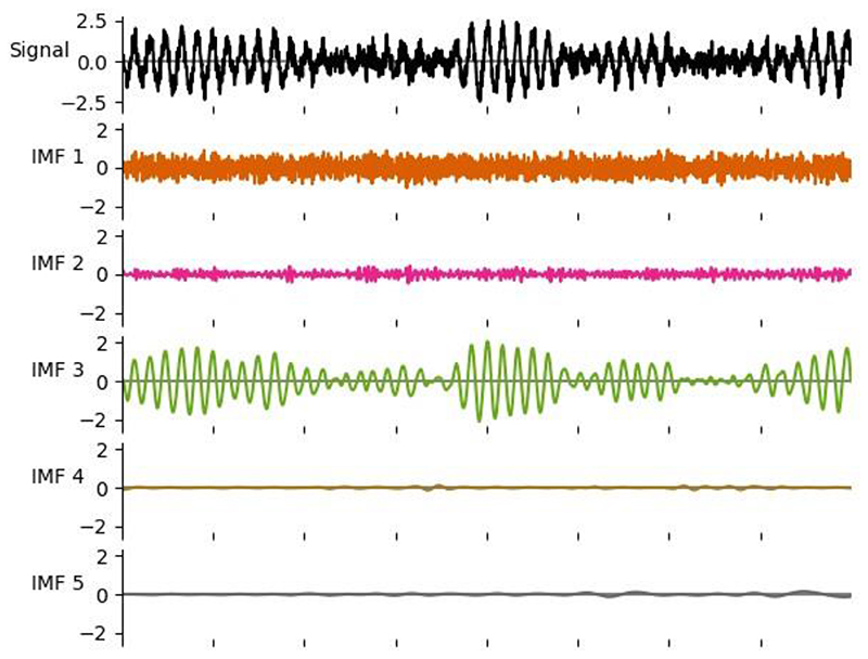
The sift algorithm is implemented in the emd.sift module, including the classic sift (emd .sift.sift; Huang et al. (1998)), the Ensemble EMD (emd.sift.ensemble_sift; Wu & Huang (2009)), Masked EMD (emd.sift.mask_sift; Deering & Kaiser (2005)) and the second-level sift (emd.sift.sift_second_layer; Huang et al. (2016)). The ensemble and masked sift variants can be optionally accelerated by parallel processing (though this is not possible in all variants of the sift algorithm). An example set of Intrinsic Mode Functions isolated by a Masked-Sift is shown in Figure 1. The sift functions rest upon a range of lowerlevel utility functions, which can be customised and used directly if needed. All levels of the sift computation are customisable from the top-level sift functions. Users can configure these sift options using a dictionary-like emd.sift.SiftConfig object. This config can then be passed directly to the sift functions or saved in YAML format for later use or sharing.

Figure 1. A simulated signal with an oscillatory component (black line - top panel) with a set of intrinsic mode functions estimated using a mask sift EMD (coloured lines - lower panels).

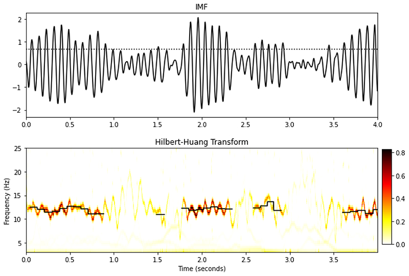
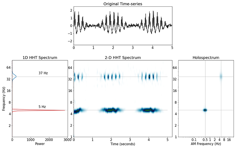
Each IMF can be analysed in terms of its instantaneous frequency characteristics at the full temporal resolution of the dataset (Huang et al., 2009). The Hilbert transform is used to construct an energy-frequency or energy-frequency-time spectrum known as the HilbertHuang Transform (HHT). A second level decomposition of the amplitude modulations of each IMF extends the HHT to the Holospectrum, describing signal energy across carrier frequency, amplitude modulation frequency and time (Huang et al., 2016). The frequency transforms are implemented in the emd.spectra submodule. emd.spectra.frequency_stats implements a set of methods for computing instantaneous frequency, phase and amplitude from a set of IMFs. These can be used as inputs to the emd.spectra.hilberthuang or emd.spectra .holospectrum to obtain energy distributions across time and frequency (see examples in Figures 3 and 4). The Hilbert-Huang and Holospectrum computations can be very large, so these functions use an efficient sparse array implementation.

Figure 3.

Top panel: An Instrinsic Mode function from a simulated signal (black line) and an amplitude threshold (dotted line). Bottom Panel: 2D Hilbert-Huang Transform. Darker colours indicate greater power and the black lines indicate cycle average instantaneous frequency of large amplitude cycles.

Figure 4.

Top panel: A segment of a simulated containing two nested oscillations and white noise. One 5Hz oscillation with 0.5Hz amplitude modulation and a 37Hz signal whose amplitude is modulated by the lower-frequency 5Hz oscillation. Bottom left: The 1D Hilbert-Huang transform of this signal. Bottom Center: The 2D Hilbert-Huang transform. Bottom Right: The Holospectrum.

The EMD toolbox provides a range of functions for the detection of oscillatory cycles from the IMFs of a signal. Once identified, each cycle can be characterised by a range of features, including its amplitude, frequency and waveform shape. Tools are provided for detecting continuous chains of oscillatory cycles and for matching similar cycles across datasets. The cycle analysis functions are implemented in emd.cycle.

A range of utility and support features are included in the EMD toolbox. Firstly, a customisable logger (implemented in emd.logger) is threaded throughout the toolbox to provide progress output about ongoing computations, warnings and errors. The logger output may be augmented by the user and any output can be directed to a specified log file in addition to the console. Secondly, EMD is supported by a range of tests, implemented in the py.test framework. These include both routine usage tests and tests ensuring that the behaviour of the sift routines meet a set of pre-specified requirements. Finally, emd.support contains a set of functions for running tests and checking which versions of EMD are currently installed and whether updates are available on PyPI.

Target Audience

Since its initial publication in 1998, the EMD approach has had a wide impact across science and engineering, finding applications in turbulence, fluid dynamics, geology, biophysics and neuroscience amongst many others. The EMD toolbox will be of interest to scientists, engineers and applied mathematicians looking to characterise signals with rich dynamics with a high temporal and spectral resolution.

State of the field

The popularity of the EMD algorithm has led to several implementations which offer overlapping functionality. Here we include an incomplete list of these toolboxes providing sift, ensemble sift and HHT implementations. In Python there are two substantial EMD implementations available on the PyPI server: PyEMD (Laszuk, 2017) and PyHHT (Deshpande, 2015). Each of these packages implements a family of sifting routines and frequency transforms. Another implementation of EMD, in Matlab and C, is available from Patrick Flandrin (Flandrin, 2007). This provides a wide range of sift functions, but limited frequency transform or spectrum computations. Finally, the basic EMD algorithm and HHT is implemented in the MatLab signal processing toolbox (The MathWorks, 2019).

The EMD toolbox covers much of the functionality in these packages within a single computational framework. Beyond these methods, we add fully-featured implementations of masked sift and second-level sift routines, as well as the first Python implementation of higher-level Holospectrum analyses. Finally, we offer a suite of tools designed for analysis of single-cycles of an Intrinsic Mode Function.

Installation & Contribution

The EMD package is implemented in Python (>=3.5) and is freely available under a GPL3 license. The stable version of the package can be installed from from PyPI.org using pip install emd. Users and developers can also install from source from gitlab. Our documentation provides detailed instructions on installation and a range of practical tutorials. Finally, users wishing to submit bug reports or merge-requests are able to do so on our gitlab page following our contribution guidelines.

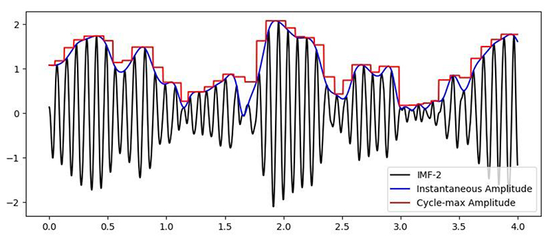
Figure 2. A segment of a simulated signal with its instantaneous amplitude and a time-series containing the maxiumum amplitude of each successive cycle.

References

- Deering R, Kaiser JF. The use of a masking signal to improve empirical mode decomposition. Proceedings. (ICASSP 05). IEEE International Conference on Acoustics, Speech, and Signal Processing, 2005; 2005. [DOI] [Google Scholar]
- Deshpande J. pyHHT. 2015 https://pyhht.readthedocs.io/en/latest/index.html; readthedocs.
- Flandrin P. Matlab/c codes for EMD and EEMD with examples. 2007 http://perso.enslyon.fr/patrick.flandrin/emd.html.
- Huang NE, Hu K, Yang ACC, Chang H-C, Jia D, Liang W-K, Yeh JR, Kao C-L, Juan C-H, Peng CK, Meijer JH, et al. On Holo-Hilbert spectral analysis: A full informational spectral representation for nonlinear and non-stationary data. Philosophical Transactions of the Royal Society A: Mathematical, Physical and Engineering Sciences. 2016;374(2065):20150206. doi: 10.1098/rsta.2015.0206. [DOI] [PMC free article] [PubMed] [Google Scholar]
- Huang NE, Shen Z, Long SR, Wu MC, Shih HH, Zheng Q, Yen N-C, Tung CC, Liu HH. The empirical mode decomposition and the Hilbert spectrum for nonlinear and non-stationary time series analysis. Proceedings of the Royal Society of London Series A: Mathematical, Physical and Engineering Sciences. 1998;454(1971):903–995. doi: 10.1098/rspa.1998.0193. [DOI] [Google Scholar]
- Huang NE, Wu Z, Long SR, Arnold KC, Chen X, Blank K. On Instantaneous Frequency. Advances in Adaptive Data Analysis. 2009;01(02):177–229. doi: 10.1142/s1793536909000096. [DOI] [Google Scholar]
- Laszuk D. Python implementation of empirical mode decomposition algorithm. GitHub Repository. 2017 https://github.com/laszukdawid/PyEMD; GitHub.
- The MathWorks, Inc. EMD implementation in the matlab signal processing toolbox. 2019 https://www.mathworks.com/help/signal/ref/emd.html.
- Wu Z, Huang NE. Ensemble Empirical Mode Decomposition: A Noise-Assisted Data Analysis Method. Advances in Adaptive Data Analysis. 2009;01(01):1–41. doi: 10.1142/s1793536909000047. [DOI] [Google Scholar]