CHESS enables quantitative comparison of chromatin contact data and automatic feature extraction

Abstract

Dynamic changes in the three-dimensional (3D) organization of chromatin are associated with central biological processes such as transcription, replication, and development. The comprehensive identification and quantification of these changes is therefore fundamental to our understanding of evolutionary and regulatory mechanisms. Here, we present CHESS (Comparison of Hi-C Experiments using Structural Similarity), an algorithm for the comparison of chromatin contact maps and automatic differential feature extraction. We demonstrate the robustness of CHESS to experimental variability and showcase its biological applications on: i) inter-species comparisons of syntenic regions in human and mouse; ii) intra-species identification of conformational changes in Zelda-depleted Drosophila embryos; iii) patient-specific aberrant chromatin conformation in a diffuse large B-cell lymphoma sample, and, iv) the systematic identification chromatin contact differences in high-resolution Capture-C data. In summary, CHESS is a computationally efficient method for the comparison and classification of changes in chromatin contact data.

Introduction

Eukaryotic genomes follow similar global organizational principles: a multi-layer, hierarchical organization into domains, with specific 3D interactions between individual genomic regions¹. Local chromatin conformation, however, can be variable across species^2–6, developmental stages^7–9, cell types^10,11, and can change dynamically with transcription¹², during replication¹³, and cell division¹⁴, among other contexts. Mutations affecting nuclear architecture have been shown to cause misregulation of gene expression leading to developmental disorders and disease (reviewed in ^15,16). It is therefore important to elucidate the relationship between nuclear architecture, evolution, and fundamental biological processes.

Existing approaches to identify changes in the 3D conformation of genomic regions have relied partially on visual analysis of differences, such as a side-by-side evaluation of Hi-C matrices^17,18 or fold-change maps¹⁹. While visual comparisons can highlight specific changes in Hi-C matrices, results are often difficult to quantify and, by nature, cannot be automated to compare large numbers of matrices. More quantitative approaches have been developed. One class of tools focuses on the assessment of the degree of similarity or reproducibility between full chromatin contact matrices / datasets and does not allow for the identification of regions with particularly strong similarities or differences^20–24. Another focuses on the comparison of specific features, such as topologically associating domains (TADs)^25,26, or loops^10,27, which limits the discovery of differences to the specific feature analyzed. A third class of tools aims to find single pairs of bins with significantly differential interactions^28–32 without providing any information about the specific type of structural feature that changes. Therefore, there is a need for methods that allow a systematic comparison of the 3D conformation of genomic regions, that is at the same time quantitative, able to identify and classify a range of structural variations, and corresponds well to the visual perception of differences.

Here, we describe CHESS, an algorithm to robustly identify and classify specific similarities or differences and features in chromatin contact data using a feature-free approach. CHESS applies the concept of the structural similarity index widely used in image analysis^33,34 to chromatin contact matrices, assigning a structural similarity score and an associated P value to pairs of genomic regions. Next, CHESS uses image processing approaches to automatically extract 3D chromatin conformation features, such as TADs, stripes or loops. We first demonstrate the robustness of CHESS scores by evaluating the method on artificially generated and real Hi-C matrices of different sizes, sequencing depths, and varying levels of noise. We then highlight the utility of CHESS in different real-world applications: i) genome-wide comparisons of syntenic regions between human and mouse; ii) the detection of conformational changes in Drosophila melanogaster upon knockdown of the transcription factor Zelda during early embryonic development; iii) the detection of 3D chromatin conformation changes in B-cells of a diffuse large B-cell lymphoma (DLBCL) patient; and, iv) the automatic detection and classification of subtle changes in chromatin conformation from genome editing experiments. Overall, our results demonstrate that CHESS can be successfully applied to diverse chromatin contact datasets to quantitatively determine structural differences between them.

Results

Overview of the CHESS algorithm

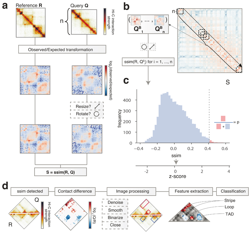
CHESS assesses the degree of similarity between any pair of normalized chromatin contact matrices, such as those produced from Hi-C, or tiled Capture-C experiments (Fig. 1a). It provides a measure for quantifying matrix similarity, which allows the identification of particularly similar or dissimilar pairs. There are very few limitations on the origin of input matrices: different regions in the same genome, the same genomic region across two experimental conditions, developmental time points, and even regions from different species. CHESS uses the structural similarity index (SSIM), a widely used metric for matrix similarity (Online Methods).

Figure 1. CHESS overview and examples.

a, CHESS workflow, showing the observed/expected transformation, size/orientation adjustments, and structural similarity score S calculation on two example matrices R and Q. b, Example of a background model for empirical calculation of z-scores and P values. Specifically, similarity scores are calculated for each n × n matrix Q^B_i at every position i along the diagonal of the whole chromosome matrix. c, Distribution of similarity scores for Q^B_i can be used to calculate P values and z-scores for S (details in Online Methods). d, Feature extraction workflow, showing the contact difference map between R and Q matrices identified by CHESS, and the list of image filters applied. The specific differential gained and lost structures are highlighted in red and blue boxes, respectively. Finally, all the features are classified according to their structural pattern, such as TADs, loops and stripes.

To calculate the similarity between a reference (R) and query (Q) matrix, their entries (i.e., contact pairs or pixels in the maps) are first divided by the expected contact intensity at the respective distance. This observed/expected transformation is necessary to remove the distance-dependency of pairwise contact probabilities characteristic of Hi-C matrices³⁵, which is otherwise the dominant topological characteristic (Extended Data Fig. 1, Online Methods). CHESS then scales the matrices to equal size and calculates the SSIM between R and Q. The SSIM score (S) is a single value, combining brightness, contrast and structure differences between two matrices (Extended Data Fig. 2). Brightness is calculated as the mean of the signal intensity. Contrast is calculated as the variance in signal. The structure term is calculated as the correlation between signal values of two matrices. S is then defined as a weighted product of these three components, which are scaled such that S ranges between −1 (inversion) and 1(identity), where S=0 indicates no similarity. We performed an in-depth evaluation of the three components of S (Extended Data Fig. 2), which showed that the main contributor to similarity when applied to Hi-C matrices is the product of contrast and structure terms.

One application of CHESS is to identify regions with strong changes in chromatin conformation between two conditions genome-wide. For this, S can be used directly to quantify changes in chromatin contacts within windows of a given size across the genome: for identical matrices S = 1, and the lower the score the larger the change (Online Methods). CHESS therefore can be used to rank genomic regions by the amount of chromatin changes within them.

An additional application of CHESS is to assess whether contact matrices originating from different genomic regions, or different genomes, are similar. An appropriate null model can be used to test whether the similarity measured by S is statistically significant. For example, a region R containing just a single TAD might obtain a high score when compared to a particular query Q, which also contains a single TAD. The same, however, is true for any region with a single TAD, which is why the similarity of R and Q is not particularly special in this instance. The score for the comparison of R vs. Q should then be assigned a low significance. Conversely, when two highly complex regions with many structural features are assigned a strong similarity score S, it is unlikely to find an equally similar region in the genome by chance, and the comparison is given high statistical significance. To compute a suitable null model, CHESS compares the reference matrix R to all other regions of the same size across the genome (referred to as Q^B_i in Fig. 1b). The distribution of scores from the null model is then used to calculate a z-score, corresponding to a normalized effect size, and a P value, denoting the frequency of scores equal to or higher than S in the null model (Fig. 1c, Online Methods). Therefore, CHESS enables a quantitative comparison and assessment of statistical significance of contact matrix similarities.

Automatic feature selection and classification of structural changes

In addition to the identification of changes in chromosome conformation data, a major analytical task consists in the recognition of changes in specific 3D chromatin organization features, such as TADs, among others. To specifically determine which features change between a pair of samples, CHESS implements a simple and fast workflow of image filters that allow their automatic identification and classification (Fig. 1d). First, a differential contact matrix is computed for each CHESS comparison, and gained and lost contacts in each matrix are separated for further analysis. Second, the matrices are denoised, smoothed and binarized to apply a close morphology filter to extract the individual areas changing in each comparison. Subsequently, the 2D cross-correlation between all the extracted areas in a dataset is computed. Finally, K-means clustering is used to detect the main structural features identified in these areas (Fig. 1d). Overall, this strategy allows one to automatically identify the precise 3D structural features, such as TADs, loops and stripes, which are changing in a particular region.

CHESS requires only low sequencing depth and tolerates a high level of noise

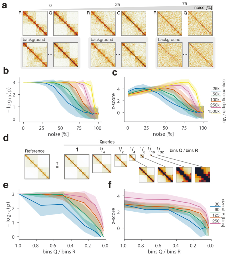
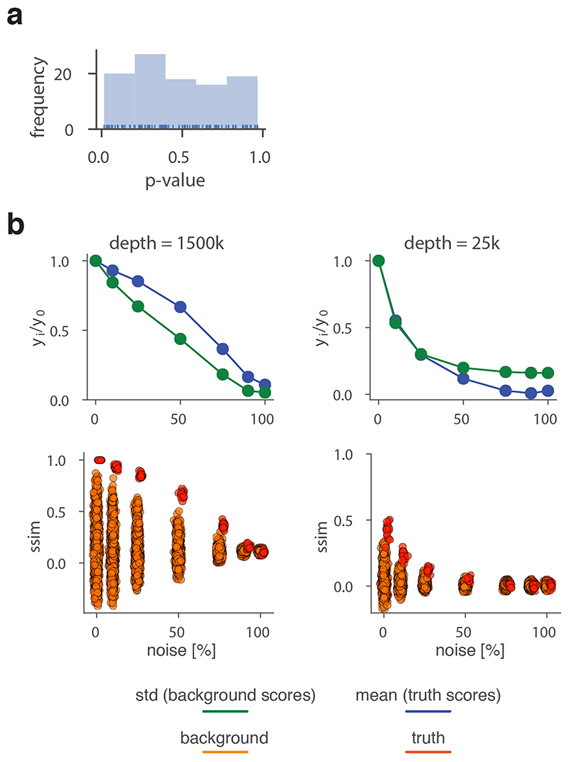
To robustly estimate the performance of CHESS with regards to different experimental conditions (e.g., noise, sequencing depth) and matrix parameters (e.g., size, size difference), we generated a set of synthetic Hi-C data designed to reflect features commonly observed in real-world Hi-C matrices, including an exponential decay of contact frequency with genomic distance, TADs, and loops (Online Methods). To test the sensitivity of CHESS to noise and sequencing depth, we compared an artificial matrix R to a copy Q of itself, while adjusting the sequencing depth and adding noise to both of the matrices independently. As a background to calculate P values and z-scores, similarity scores were additionally calculated in comparisons of R to 1,000 randomly generated artificial matrices at the same sequencing depth and noise level (Fig. 2a). These simulations show that Q is correctly assigned the best CHESS score for “deeply sequenced” matrices up to a noise level of 90% (Fig. 2b). Beyond that, ranking quickly becomes random, which is reflected in a uniform distribution of P values (Extended Data Fig. 3). For artificial matrices with fewer contacts, CHESS still tolerates noise levels of 60-80%. Correspondingly, z-scores are consistently high for the same levels of noise depending on sequencing depth (Fig. 2c). Interestingly, z-scores do not peak at 0% noise. This can be explained by the changing standard deviations of the background scores: with increasing noise, the similarity of random matrices increases, leading to progressively narrower distributions of CHESS scores. This leads to a slight increase in z-scores up until the point that CHESS is no longer able to identify Q as the top-ranking hit in these comparisons (Extended Data Fig. 3).

Figure 2. CHESS evaluation on synthetic Hi-C matrices.

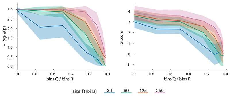
a-c, Tests for the tolerance of CHESS to increasing levels of simulated experimental noise. a, Schematic representation of the tests for the sensitivity of CHESS to noise. b, Empirically determined CHESS P values on synthetic matrices with increasing levels of noise (details in Online Methods). c, CHESS z-scores on synthetic matrices with increasing levels of noise. d-e, Tests for the performance of CHESS when comparing matrices of different sizes. d, Schematic representation of different scaling factors used to generate a query matrix Q from a reference R. e, Dependence of CHESS P values on the scaling factor of synthetic matrices Q and R. f, Dependence of CHESS z-scores on the scaling factor. b, c and e, f, Solid lines indicate the mean, shaded areas the standard deviation over 100 simulations per parameter combination. Lowest possible P value in all tests: 0.001.

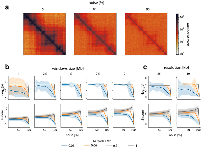
To verify these results in a real-world setting, we repeated the above analyses on a deeply sequenced mouse embryonic stem cell (mESC) Hi-C dataset¹². Interestingly, the results on real data indicate an even higher robustness of CHESS to high noise and low sequencing depth than observed on synthetic datasets; while high robustness requires sufficiently large region sizes (> 2.5 Mb, which is likely due to the increased amount of distinctive features in larger regions), CHESS tolerates sequencing depths as low as 0.06 M/Mb and 80% noise (Extended Data Fig. 4), demonstrating the applicability of this approach in shallow-sequenced datasets. The increased robustness to noise is likely due to a stronger signal enrichment in structural features, compared to the artificial data, since structural features remain visible by eye even at 95% noise (Extended Data Fig. 4). Additionally, CHESS results are highly robust to parameter changes, including comparison window span, step size, matrix resolution, and sequencing depth (Extended Data Fig. 5, Online Methods). Overall these results demonstrate the ability of CHESS to reliably detect similarities between Hi-C matrices even at very low sequencing depths and with high amounts of noise.

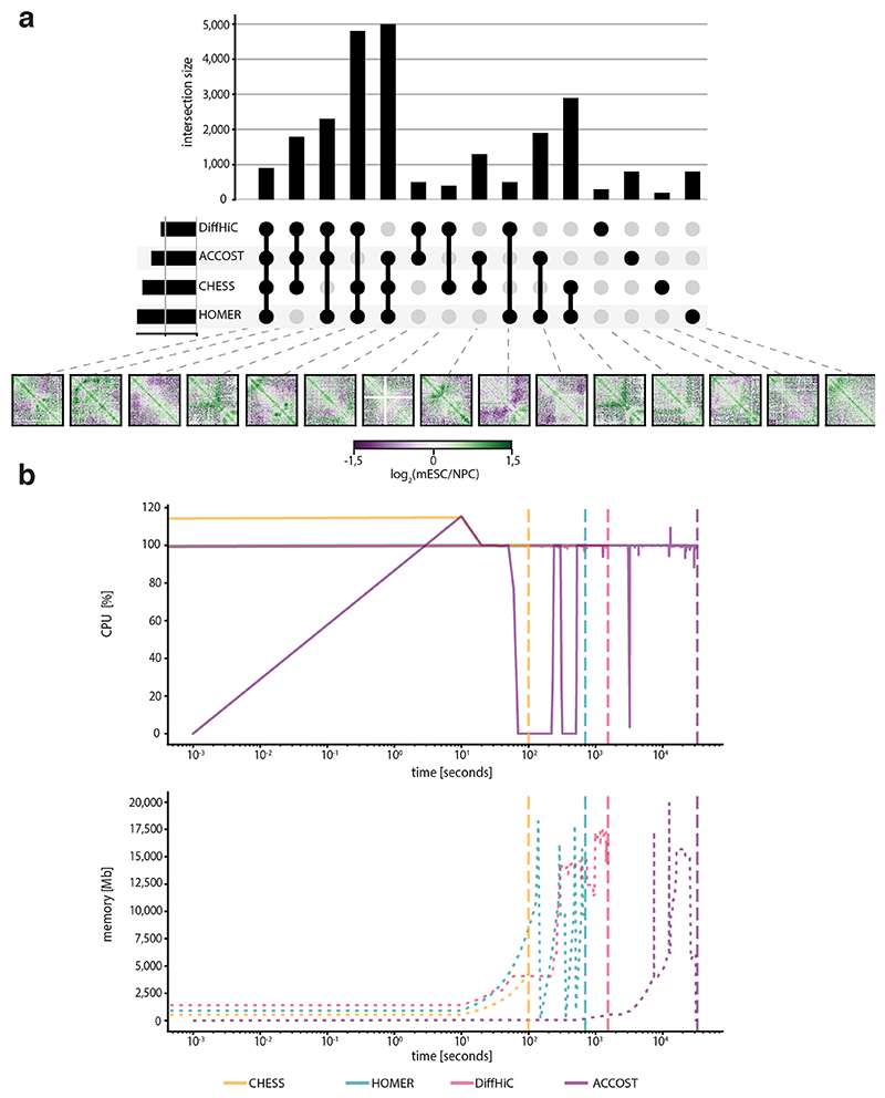
Finally, to benchmark CHESS, we compared it to three widely used differential interaction detection packages: HOMER³², diffHiC³⁰ and ACCOST³¹. All methods were run using default parameters on Hi-C interaction matrices at 5-kb resolution for chromosome 19 from mESCs and NPCs (neural progenitor cells)¹². Since a gold-standard for assessing accuracy of differential chromatin interactions does not exist, we performed the analysis by examining the degree of overlap in differential interacting regions identified by the three methods. Overall, we find a high level of overlap (Extended Data Fig. 6). However, it is important to note that CHESS identifies entire regions with differences while diffHiC, HOMER and ACCOST identify specific pairs of bins with significant differences in contact counts. A small proportion of differences were reported only by HOMER, diffHiC and ACCOST. Importantly, many of these differential interactions were filtered out by CHESS due to low signal to noise ratios.

Together, these results demonstrate that CHESS is able to robustly identify changes in chromatin conformation features over a wide range of experimental conditions.

CHESS similarity scores are consistent for matrices of different sizes

An immediate advantage of the analytical strategy behind CHESS is that it allows the calculation of S for matrices of different sizes. This is needed to measure, for example, the similarity between Hi-C maps of different species, or for paralog-containing regions within the same genome. To do so, we implemented an upscaling transformation of the smaller of the two matrices (in case these are of different sizes) using nearest-neighbor interpolation (Online Methods). To test the performance of CHESS on matrices of different sizes, we calculated S using an artificial matrix R and a matrix Q that maintains the relative positions, sizes and intensities of all features in R (i.e., TADs and loops), but differs in size by a certain scaling factor (Fig. 2d, Supplementary Fig. 1, Online Methods). Randomly generated matrices of the same size as Q serve as background to calculate statistical significance. In a “deeply sequenced” Hi-C matrix of 1.5 M/Mb, divided into equally sized regions of at least 60 bins, CHESS consistently ranks Q as the matrix most similar to R even if Q is less than half the size of R (Fig. 2e, f). Small matrices Q (smaller than 30 bins) do not rank higher than random matrices, since they do not provide enough space to fit the features (i.e., TADs and loops) of the reference matrix. A test with a simulated sequencing depth of 100 k/Mb and 25% noise led to similar results, demonstrating that the method’s ability to detect similarities between matrices of different sizes is robust to experimental noise and different levels of sequencing depth (Extended Data Fig. 7).

Comprehensive ranking of syntenic regions by structural similarity

Having validated the ability of CHESS to reliably and robustly detect similarities and differences between synthetic and real Hi-C matrices, we next showcase its use in a real research scenario. Previous studies have examined the level of chromatin conformation similarity for regions of synteny (highly conserved sequences between species) finding a high degree of structural conservation between them^2,10,18. These comparisons have mainly focused on visual examination of individual examples^10,18, correlation analyses of specific 3D genome features, such as the binding of architectural proteins², measures of insulation³⁶, or the contact strength correlation within syntenic regions². However, a genome-wide quantification of the degree of similarity at the contact matrix level is lacking.

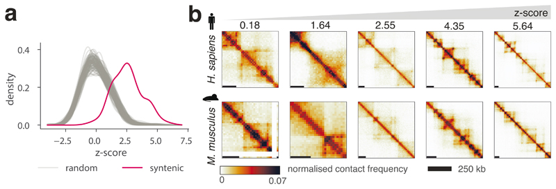
We used CHESS to determine the level of chromatin conformation conservation for 175 regions of synteny between human and mouse obtained from Synteny Portal³⁷. To calculate statistical significance for the degree of conservation, we computed S scores for 100 random permutations of syntenic region pairs. Similarity scores for true syntenic region pairs were strongly and consistently higher than those of random pairs (Fig. 3a, P = 0.01; permutation test). Therefore, in agreement with previous observations^2,10,18, these results demonstrate genome-wide that overall, regions of synteny between human and mouse share a similar 3D chromatin organization. However, our results highlight that not all regions of synteny have the same degree of structural similarity (Fig. 3b), suggesting that the evolutionary constraints on 3D chromatin structure are not uniform across the genome, resulting in different rates of evolution. In summary, our results demonstrate that CHESS can be used to automatically quantify and rank 3D structural similarity genome-wide between species.

Figure 3. Global comparison of syntenic region similarity between human and mouse using CHESS.

a, Distributions of empirically determined CHESS z-scores for 175 syntenic region pairs in human and mouse (red) and 100 random permutations of region pairs (grey) (details in Online Methods). One sided randomization test P value = 0.01, comparing the mean scores of randomly permuted pairs to the mean score of real syntenic regions. b, Examples of syntenic regions with increasing CHESS z-scores from left to right.

Detection of structural variation upon genetic perturbation

A common problem in comparative genomics is the detection of emerging changes in a system with different experimental conditions, including targeted introduction of disturbances into the system. When applied to chromatin conformation, this approach has been fundamental to determine the contribution to 3D chromatin organization of different factors, such as CTCF, cohesin or WAPL, among others^38–43. However, these studies mostly relied on the detection of visual differences between Hi-C maps or the comparison of measurements derived from these maps, such as the directionality or insulation indices.

Using the insulation score¹⁹, a metric that is low at TAD borders and high within TADs, we have previously shown that depletion of the pioneer transcription factor Zelda during early embryonic development in Drosophila leads to a weakening of insulation at TAD boundaries in loci strongly bound by Zelda in wild type embryos⁹. Therefore, we sought to evaluate the sensitivity of CHESS in detecting these changes, as well as its ability to detect further modifications in chromatin conformation that would have escaped detection by a simple comparison of insulation scores.

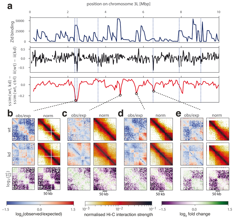
Running CHESS in a comparison between wild type nuclear cycle 14 and Zelda-depleted embryos resulted in the detection of 65 regions in the genome with changes in chromatin conformation. Out of the 62 differential boundaries identified before⁹, 29 were contained in regions marked as changing by CHESS. Visual inspection of the structural changes at the remaining 33 differential boundaries revealed that the differences in contact intensities were typically small and primarily caused by a decline in short distance contacts around the boundary (Supplementary Fig. 2. We reasoned that a smaller matrix size should increase the sensitivity of CHESS with regards to these types of changes, since they would correspond to a larger fraction of the input matrix pixels. Indeed, after reducing the size of the input matrices from 250 kb to 125 kb, we detected 51 out of 63 differential boundaries as changing, along with 163 additional regions. It is important to note that this approach is likely to miss changes occurring far away from the diagonal, such as differences in the contact probability decay, long-range loops, or large TADs. Therefore, we conclude that, by altering the size of compared matrices, it is possible to fine-tune CHESS to the scale of changes it can detect.

Visual examination of the regions captured in the first run, as well as of control regions, confirmed the detected differences. Notably, besides the already reported loss of insulation at a subset of Zelda-bound TAD boundaries (Fig. 4a)⁹, the newly identified regions highlighted a range of structural changes, such as differing signal intensity away from the main diagonal of the Hi-C matrix, suggesting changing levels of chromatin compaction, and varying contact intensities inside TADs and at long distances (Fig. 4b-e). These results demonstrate that CHESS is able to systematically identify regions that undergo structural changes upon genetic perturbation, covering a broad spectrum of structural features, which correspond well to visual perception of differences.

Figure 4. Identification of chromatin conformational changes in fly embryos after Zelda (zld) knockdown.

a, Zelda binding signal in wild type (wt) (top), insulation score difference between wt and zld knockdown (kd) (middle, smoothed), and difference between similarity scores calculated on wt to kd and wt to water injection control (ctrl) (bottom) for regions on a subset of chromosome 3L. Dotted blue lines indicate differential boundaries as identified by ⁹. b-e, Examples of regions with the strongest conformational changes between wt and kd, showing observed/expected (obs/exp) and normalized Hi-C matrices, and log₂-fold-change matrices for wt/kd. White lines on the Hi-C plots correspond to regions of the genome masked from the analysis due to low mappability.

CHESS identifies structural abnormalities in diffuse large B-cell lymphoma

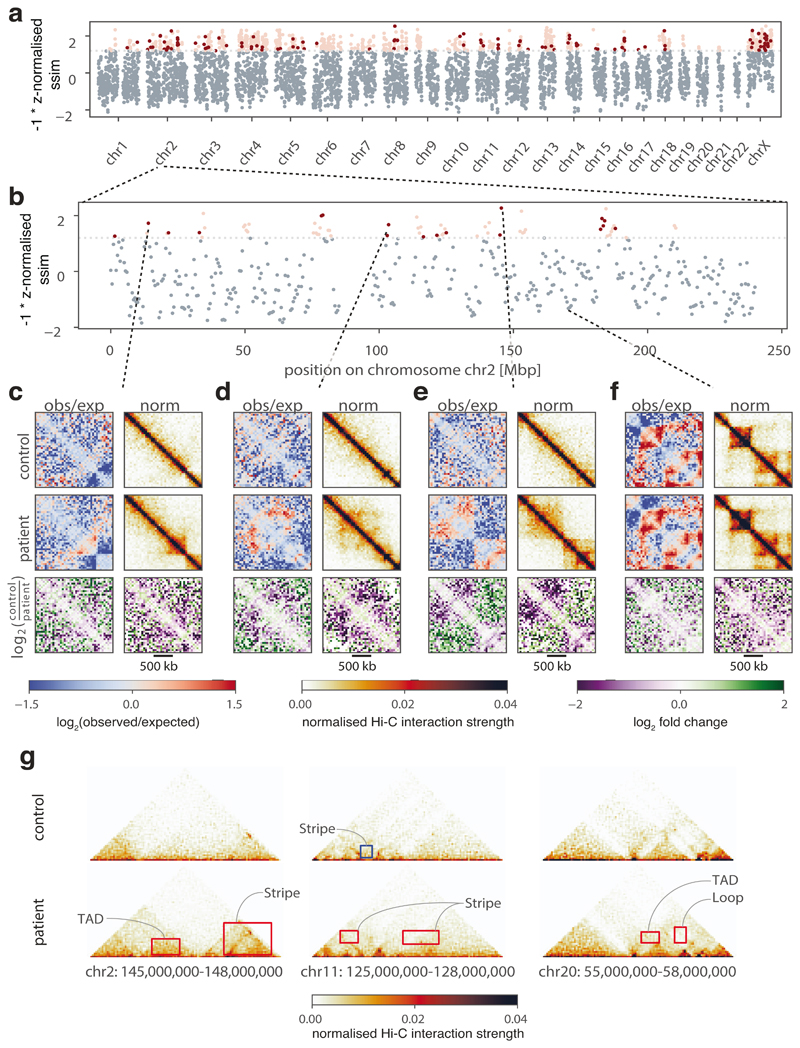
We next sought to determine whether CHESS is able to detect structural differences in clinically relevant samples. The characterization of these differences is of prime importance since changes in the 3D structure of chromatin in mammals can have a strong impact on genomic regulation and thereby give rise to disease phenotypes^44,45 and the activation of oncogenes^46,47. We reasoned that by comprehensively scanning a genome for structural abnormalities compared to a healthy control, CHESS can greatly aid our understanding of the relationship between nuclear architecture and disease. To test this, we performed a CHESS comparison using a recent Hi-C dataset from primary diffuse large B-cell lymphoma (DLBCL) and healthy B-cells⁴⁸. Across the whole genome, CHESS identified 810 regions of 2 Mb with prominent structural variations in DLBCL (Fig. 5a, b). After filtering these for regions with high experimental noise (Online Methods), we obtained a high-confidence set of 112 regions exhibiting clear changes between healthy and diseased B-cells (Fig. 5c-e). One of the most striking examples displayed the emergence of well-defined TAD structures in a region that seemed devoid of structural features in healthy cells (Fig. 5e). Despite these differences, our analysis also revealed that the majority of structures remained unchanged (Fig. 5f). To gain further insight into the nature of the changes, we applied the feature extraction component of CHESS to the 112 selected regions. This resulted in the identification of 144 gained features (104 stripes and 40 TADs) and 53 lost loops in the DLBCL sample compared to the control (Fig. 5g). This illustrates the application of CHESS to examine disease-related processes by systematically identifying genomic regions and characterizing the specific features whose 3D structure differs between healthy and diseased cells.

Figure 5. Identification of structural changes in a diffuse large B-cell lymphoma.

a, b Similarity (z-normalized similarity score) of Hi-C data generated from healthy B-cells (control) and a diffuse large B-cell lymphoma (patient), as assessed by CHESS for 2-Mb regions. Highly dissimilar regions (z-normalized similarity score ≤ -1.2) are colored in red, where noisy regions (signal to noise ratio < 0.6) are in light red. c-f, Examples of regions with conformational changes (c-e) and conservation (f) between healthy and diseased B-cells, showing observed/expected (obs/exp) and normalized Hi-C matrices, and log₂-fold-change matrices for control/patient. g, Three examples of highly dissimilar regions identified by CHESS, with the gained and lost features highlighted in red and blue, respectively. The features are annotated according to their structural category.

Identification and automatic classification of structural features in Capture-C data

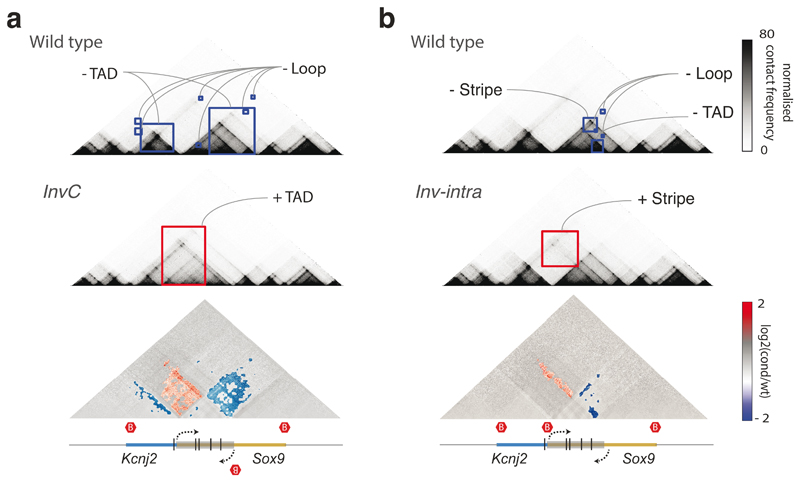
Finally, we investigated CHESS‘ ability to automatically extract features in additional types of chromatin conformation capture datasets, such as tiled Capture-C experiments⁴⁹. To do so, we analyzed previously published Capture-C experiments for CRISPR/Cas9-mediated genome edits of architectural features, such as deletion of CTCF binding sites, modifications of TAD boundaries, and a TAD inversion at the Sox9/Kcnj2 locus⁵⁰. CHESS identified all previously described 3D rearrangements in the different mutants compared to wild-type mice (Fig. 6 and Extended Data Fig. 8). In addition, CHESS identified marked differences that had not been reported in the original study. For example, besides the previously reported TAD fusion resulting from the Sox9 regulatory domain inversion (InvC), CHESS captured the loss of chromatin loops between the two TADs (Fig. 6a). A similar inversion not including the TAD boundary (Inv-Intra) did not result in a TAD fusion. However, CHESS captured an increase in contact frequencies across the boundary in the form of a stripe (Fig. 6b). Applying CHESS to all generated mutants systematically characterized the set of very subtle differences across these samples (Extended Data Fig. 8). This demonstrates that CHESS is able to automatically identify and classify chromatin contact differences.

Figure 6. Feature extraction from Capture-C data from Despang et al.⁵⁰ .

a, Feature extraction of wt against InvC mutant maps, which present an inversion in the Sox9 sequence represented by a grey box (bottom). Lost and gained structures in the mutant are highlighted in blue and red squares, respectively. The bottom plot shows a log₂ fold-change map with identified features colored according to the directionality of the change. Red hexagons demarcate the positions of TAD boundaries. b, Same as a, for feature extraction of wt against Inv-intra mutant maps, in which the same sequence is inverted, not including the border between the two TADs.

Discussion

The increasing wealth of available Hi-C datasets calls for fast, quantitative algorithms that enable a systematic comparison of local chromatin structure. However, currently there are no algorithmic approaches for Hi-C data analysis that allow automated comparisons and classification of the identified 3D genome changes directly on the matrix level. This results in a lack of identification and characterization of a broad spectrum of differences in chromatin conformation maps that can be visually recognized, but that may be missed by more specialized approaches relying on pre-processed features. We have developed CHESS to fill this gap by providing automated, systematic Hi-C matrix comparisons, and feature classification that correspond well to the visual perception of structural differences (Fig. 1). A major feature of CHESS is that it is not limited to comparing regions within a single dataset, but comparisons can be made between samples, cell types, developmental stages, and even across different species, which makes it widely applicable. We demonstrate that CHESS is robust to experimental noise and usable on shallow sequenced datasets (Fig. 2). Furthermore, we show that CHESS can be used to perform cross-species comparisons (Fig. 3) and that it is able to detect 3D genome changes in genomes of different sizes (Figs. 4-5). Finally, we demonstrate that CHESS can be used to analyze chromatin conformation capture datasets generated using different experimental approaches, such as Capture-C⁵⁰ (Fig. 6). Therefore, we expect CHESS to be immediately applicable to other datasets, including tethered chromatin conformation capture (TCC)⁵¹, digestion-ligation-only Hi-C (DLO Hi-C)⁵², genome architecture mapping (GAM)⁵³, and microscopy-based methods, such as Hi-M⁵⁴.

An additional advantage of CHESS is the fast and highly efficient implementation of the structural similarity algorithm that has a very small memory footprint, as only the two matrices that are being compared need to be loaded. As a comparison, when scanning a whole chromosome for structural differences between conditions, CHESS achieves a 4-320 times speedup at 3 times lower memory consumption compared to HOMER, diffHiC and ACCOST ^30–32 (Extended Data Fig. 6). This makes the approach usable without requiring an advanced computational infrastructure. In addition, the nature of CHESS comparisons makes them trivially parallelizable, so that the algorithm can be efficiently sped up by dedicating more computational resources to it. This allows CHESS to make the myriad of comparisons necessary for more complex biological questions, including the background computation for comparing regions of different origin.

Within this context, a promising outlook for CHESS applications is the de novo discovery of structurally similar regions between two genomes using an all-against-all comparison approach. These “structurally syntenic” region pairs could provide fundamental insights on the evolution of nuclear architecture and its 3D constraints, including the effects of processes affecting 3D chromatin organization such as rearrangements or changes in the binding of architectural proteins. Despite the efficiency of CHESS, further work and heuristics would be necessary to make this computationally tractable. Highlighting the importance of considering the 3D genome in evolutionary analyses, we find different degrees of structural conservation across mammalian evolution (Fig. 4), suggesting different rates of evolutionary change in these regions. This demonstrates how CHESS can already facilitate the study of evolutionary genomics in the context of 3D structure.

Similarly, the identification of structural variation and its association with abnormalities in 3D genome organization and gene expression misregulation is central to evaluate the contribution of chromatin organization to disease-generating processes. As a proof of principle, here we demonstrate how CHESS can be used to detect a number of chromatin conformation alterations genome-wide in B-cells from a DLBCL patient without the need of previous knowledge regarding the nature of the aberrations. Interestingly, our analysis identified regions in the genome gaining structural features, such as TADs and loops, despite the lack of protein coding genes in these regions. Instead, these regions frequently contained long non-coding RNAs and pseudogenes. Future work integrating other patient-matched genome-wide datasets, such as chromatin accessibility or RNA-seq, will be necessary to determine the cause and consequence of these changes in relation to disease.

Future improvements of CHESS might benefit from a further dissection of the structural similarity index, which may allow us to pinpoint the contributions of individual regions to overall matrix similarity. In general, structural similarity of images is an active field of research. Modifications improving the robustness of SSIM to small shifts in position⁵⁵ or its power to identify similar sub-images⁵⁶ are promising, but it remains to be determined which of the algorithms developed for assessing image similarity are compatible with the specific requirements of Hi-C matrix comparisons.

In conclusion, CHESS is an algorithm to quantitatively assess and classify the structural similarity of two genomic regions from chromosome conformation capture data – without the need for feature selection prior to comparison. CHESS is highly tolerant of differences in chromatin conformation capture library size and the noise level of datasets. Its applications include the ranking of known region pairs by similarity, such as syntenic regions in different species, and the discovery of structural changes, such as chromatin conformational changes of the same genomic region in two different conditions. CHESS has great utility in the field of chromatin conformation and can simplify the identification of disease-associated structural variation in clinical applications.

Methods

The CHESS pipeline

The CHESS pipeline is illustrated in Figure 1. CHESS takes two normalized^67,68, whole-genome Hi-C matrices as input. We recommend to use matrices at least 100 × 100 bins in size (20 × 20 is the absolute minimum allowed by CHESS) with no more than 10% of all bins unmappable (without signal). In a first step, these are transformed to observed/expected (obs/exp) matrices³⁵ by dividing each matrix entry by the average of all entries at the same distance (see below). This transformation is necessary in order to remove the distance-dependency of pairwise contact probabilities that is characteristic for Hi-C matrices. CHESS comparisons of matrices that are not corrected for this distance-dependency of contact probabilities are sensitive to varying experimental noise and relative region sizes (Extended Data Fig. 1). From the whole transformed matrices, the submatrices corresponding to the specified regions of interest are extracted, forming a comparison pair R (reference) and Q (query). Subsequently, R or Q are resized to the dimensions of the larger matrix using nearest neighbor interpolation (skimage.transform.resize in the scipy package⁶⁰). If regions are located on different strands, the matrices are rotated by 180 degrees (for example in case a syntenic region is annotated on the reverse strand). All bins marked as unmappable in either of the matrices are removed from both matrices. The resulting processed versions of R and Q are handed to the structural similarity function, yielding a raw similarity score. We use an implementation of the original structural similarity algorithm^33,34 available for the Python programming language in the scikit-image module⁶⁰. While this function was initially developed for the evaluation of image quality^33,34, it does not make any assumptions about its input data other than that it comes in the form of two matrices of same dimensionality, with numerical entries, irrespective of how the data in these matrices have been generated. Outside of the computer vision field, it is for example also used in transportation research to compare matrix representations of origin-destination graphs, which differ from chromatin contact graphs conceptually only in that they are directed graphs^69,70, and as a similarity metric for acoustic pressure signals^71,72.

In some applications, R may be compared to a pool of matrices P forming the background model. The process described above for the pair R,Q is repeated for each pair R, Q^B ∈ P. We use the similarity scores B obtained from these background comparisons to calculate a P value and a z-score for the raw score s = ssim(R,Q):

$$\begin{array}{c}p=\frac{\left|\right\{x\in B\mid x\ge s\left\}\right|}{\left|B\right|},\\ z=\frac{s-{\mu }_B}{{\sigma }_B}\end{array}$$

where μ_B denotes the mean, and σ_B the standard deviation of scores in B. We used two kinds of background models for this manuscript. (1) all submatrices of Q’s size located on the same chromosome as Q for the comparison of chromatin structures between syntenic regions, and (2) a pool of synthetic matrices built with the same parameters as Q but randomly generated features for the tests of CHESS on synthetic Hi-C data. CHESS P values are not automatically corrected for multiple testing, as this is not necessary for all use cases. If CHESS is used to identify significantly similar or different regions across the genome with a fixed acceptance threshold, the CHESS P values need to be corrected for multiple testing.

Next, CHESS extracts individual features that are different between two genomic regions (Fig. 1d). First, gained and lost contacts in the R matrix are computed and separated as increased/decreased interactions with respect to Q. Then, a set of image filters, with the parameters automatically adjusted according to the matrix size or user-defined, are applied to these two matrices that are from now on considered as images:

1. Denoise the image using a bilateral filter⁷³: this is an edge-preserving filter that averages pixels based on their spatial closeness and their radiometric similarity, by default they are computed using a window size of 3. The Gaussian function of the Euclidean distance between two pixels and its standard deviation is used to obtain the spatial closeness. The Euclidean distance between two color values is used for the radiometric similarity, CHESS by default uses the mean value of the matrix. It has to be noted that higher values of spatial closeness and radiometric similarity will average the bins with larger differences.

2. Smooth the image using a median filter: this scans the image using a square shaped array with an area computed automatically depending on the picture size. This array scans the image using a windows size, and computes the median of the pixels, smoothing the signal. Higher values will smooth larger structures, while smaller values will consider more subtle signals.

3. Image binarization using Otsu’s method⁷⁴: it returns a threshold value that separates the pixels in two classes. This algorithm searches for the threshold that minimizes the intra-class variance. This threshold by default is calculated using whole matrix values to be more refined.

4. Morphological closing of the image: this filter is used to remove small dark spots and connect small bright cracks. This helps to remove the remaining noise and to enclose the individual structures. By default CHESS uses a square of 8 bins, higher values will enclose larger structures while lower will consider smaller or more punctuated signals.

With the four filters, CHESS extracts individual structures, which can be used to get the main structural clusters according to their pattern of interactions. First, the 2D cross-correlation between all the individual features is computed. Finally, the K-means clustering algorithm is applied to obtain the main structural clusters. The optimal number of clusters is computed according to the elbow method by fitting the model within a range of 1 to 15 clusters, which may vary depending on the number of identified differential features. The robustness of the clustering was assessed by downsampling the identified structural features from the Hi-C data generated from healthy B-cells (control) and a diffuse large B-cell lymphoma (patient) and computing the optimal number of clusters. This process was repeated 1,000 times. The clustering step proved to be highly robust to data sparsity (Supplementary Fig. 3).

Calculation of observed/expected matrices

We calculated the observed /expected form M^obs/exp of a balanced matrix M by first computing the expected matrix M^exp by determining the average value of each diagonal in M:

$$M^{{\exp }_{i,j}}=\frac{{\displaystyle {\sum }_{n=1}^{N-D}{M}_{D+n,n}}}{N-D}\text{ with }D=i-j,i\ge j$$

As M is symmetric around M_i=j, we computed this only for i ≥ j and then set M^exp_i,j = M^exp_j,i.

We then calculated M^obs/exp:

$${{{\displaystyle M}}^{obs/exp}}_{i,j}=\frac{M_{i,j}}{{{{\displaystyle M}}^{exp}}_{i,j}}.$$

As for the matrix balancing, the observed/expected calculation was performed on a per-chromosome basis for real Hi-C data.

Generation of synthetic Hi-C matrices

To test the performance of CHESS on datasets with different sequencing depths, we generated synthetic matrices within a range of numbers of simulated read pairs. Typical numbers of valid read pairs in current Hi-C studies range from 0.1 million per megabase (M/Mb)^10,18 to 1 M/Mb¹². As an example of a deeply sequenced dataset, we generated matrices with an equivalent depth of 1.5 M/Mb, corresponding to ~4.5 billion mapped reads across the whole genome in a Hi-C experiment on human cells. Datasets at lower sequencing depths were then generated by downsampling the number of read pairs in the original matrix by randomly removing pairs of contacts (Supplementary Fig. 4) (Online Methods). This ensures that the overall structure of the dataset is maintained for the evaluation of sequencing depth-related effects. In addition, experimental noise was also simulated in the synthetic datasets by removing a number of contacts and adding them at random locations (Supplementary Fig. 4). This allows us to model the effect of random ligations, a main contributor to noise in chromatin contact maps.

To generate a synthetic matrix, we performed the following steps: first, we produced an empty matrix M of dimensions n². We then filled M with simulated pairs of reads, modeling the power-law decay of signal away from the main diagonal^35,75 by:

$$x_i={{(10}^{-4}+\frac{1-{10}^{-4}}{1000}i)}^{-0.85},i=0,1\dots ,n$$

where x_i denotes the read counts at the ith diagonal, counted as moving away from the main diagonal at i = 0. At this point, the number of reads is uniform in each diagonal and the mean number of reads per bin is inversely proportional to the matrix size. We then added structural features resembling TADs and loops to M.

First, three layers of TADs were added. TAD size was randomly determined by drawing a size s from a truncated normal distribution, while TAD intensity was modelled by adding a constant read count to a square of area s². For each consecutive layer the TAD size decreased while the TAD intensity increased (Supplementary Table 1). To start with, we placed a first TAD at a randomly chosen position on the main diagonal at least 0.1n away from each end of the diagonal. We then filled the main diagonal to both sides of this initial TAD with adjacent TADs. In cases where a space smaller than the lower bound of the truncated normal occurred at the ends of a diagonal, we covered it by adding a small TAD that can be thought of as being part of a bigger TAD reaching into the field of view from an adjacent genomic region. In the second and third round, smaller TADs were placed inside the TADs generated in the previous round.

Second, corner loops were added to TADs with a chance of 1/3. Loops were modelled as squares with an additional, randomly selected intensity of either 90%, 140% or 220% of the intensity and side lengths of either 5%, 7%, or 10% of the side length of the corresponding TAD.

Simulation of different sequencing depths and experimental noise

Hi-C matrix quality and resolution are primarily affected by two properties: (1) random ligations, which are distinct from proximity ligations; and (2) sequencing depth. These properties have distinct effects: random ligations are an indicator of poor library quality and introduces “noise” into the Hi-C matrix, while sequencing depth determines the achievable matrix resolution. However, they are not entirely independent. Increased sequencing depth can mitigate the effects of random ligations by enriching contacts in regions with “true” proximity signal.

In all our tests of CHESS, lower sequencing depths were simulated by subsampling, i.e. the random removal of “ligation fragment” pairs in a high-resolution matrix. Random ligations, on the other hand, were simulated by the random replacement of pairs in a matrix. In particular, to model different sequencing depths, we lowered the density of read pairs in M by removing random read pairs until we reached the desired number of read pairs d. Subsequently, we simulated an experimental noise level ε by reassigning r = ε × d read pairs to randomly selected pairs of loci.

As stated above, our noise models random ligations in the Hi-C experiment that can occur after the genomic material has been digested. These random ligations are intramolecular ligations (not within a crosslinked pair). The probability of a random ligation of two fragments is therefore not related to the linear genomic distance between them. In consequence, the distance decay graph is expected to approach a flat line as the fraction of random ligations in the Hi-C library increases. Our noise procedure moves a fraction of the reads in each bin to randomly chosen bins, where each bin in the map has the same chance of receiving a read. This procedure results in the expected behavior of the distance decay graph, as shown in Supplementary Figure 5.

The downsampling procedure on the other hand removes randomly chosen reads, without adding them anywhere. As the fraction of reads removed is on average the same at all genomic distances, the distance decay graph does not change significantly due to sampling. Slight deviations occur only close to the maximum distance, where the numbers of reads and bins are small enough to allow for random fluctuations of the mean after sampling. We show the largely unchanged distance decay in Supplementary Figure 5.

We simulated the size difference of regions with similar structural features by first generating a reference matrix of a certain size n_r and saving the relative positions and intensities of structural features in it. We then generated query matrices of smaller sizes n_q and placed the structural features at the same relative positions (rounded to the next full bin) with the same intensities. To ensure equal sequencing depth relative to the matrix size between the scaled matrices, we subsequently adjusted the depth of the scaled matrices to a scaled depth d_q) in relation to the depth of the reference matrix d_r:

$$d_q=d_r\frac{n_q}{n_r.}$$

The structural similarity algorithm in chromatin contact map comparisons

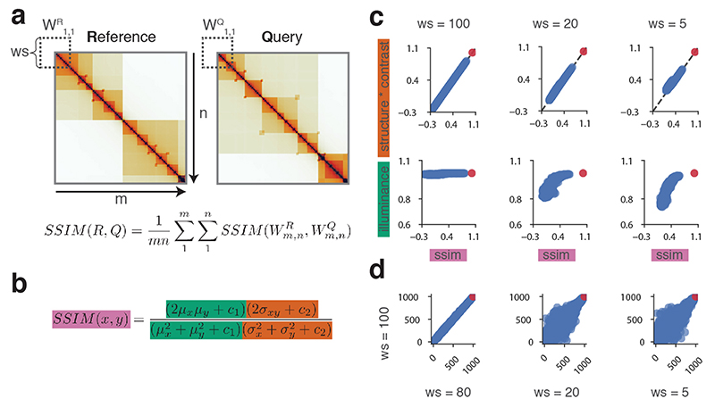
The SSIM score for whole matrices can be calculated from the average of multiple “sub-scores” obtained on smaller subsets of a matrix, the size of which can be controlled with dedicated window size parameters (Extended Data Fig. 2). Each sub-score consists of three components: corrections for illuminance (differences in brightness), corrections for contrast, and the correlation coefficient between the two matrices (Extended Data Fig. 2)^33,34. By default, CHESS does not use sub-scores, but computes a single SSIM value for the whole matrix comparison immediately.

We quantified the contribution of each component to the final score in comparisons of a random synthetic Hi-C reference matrix to an identical copy of itself and to a pool of 1,000 randomly generated matrices of the same size. We assessed the dependence of the final score on each component using multiple window sizes (Extended Data Fig. 2). For sufficiently large window sizes, SSIM sub-scores are perfectly reflected by the combination of the contrast and correlation components. Only for very small window sizes does the illuminance play a minor role. While different window sizes affect the scores and relative rank of random matrices (Extended Data Fig. 2), the comparison of the reference matrix to its identical copy yields a perfect score in all comparisons, independently of the window size.

Tests on synthetic Hi-C matrices

We tested CHESS on synthetic matrices in two main test scenarios: noise/sequencing depth tests and size/size difference tests. The test setup was similar in both scenarios. For each test run, we first defined the test conditions by setting the following parameters: the size of reference matrices, query matrices, the reference noise level, query noise level and the sequencing depth (always the same for reference and query), the type of the input matrices (normalized or observed/expected), and the window size parameter of the structural similarity function. Using these parameters, we then generated a reference set of 100 synthetic Hi-C matrices. Corresponding to these references we then produced 100 query matrices, differing in a certain parameter (noise level or size) by a certain factor, but with the same structural features in the same positions (see ‘Generation of synthetic Hi-C matrices’). We then generated a decoy pool of 1,000 synthetic matrices with all parameters equal to the query matrices, but with randomly generated features. Each reference matrix was compared to its corresponding query using the structural similarity algorithm with the specified parameters, and also to each matrix in the decoy pool, which we used as a simulation of the genomic background. The p and z-scores were then calculated as described in ‘The CHESS pipeline’. The best possible P value in this test $\left(P\le \frac{1}{1000}\right)$ was achieved when the comparison score of R vs. Q was greater than all scores from comparisons to the 1,000 random matrices.

Processing of Hi-C matrices

We obtained Hi-C sequencing reads for human IMR90¹⁰, mouse CH12.LX¹⁰ (GSE63525), mouse ESCs and NPCs¹², and fly embryos at nuclear cycle 14, in wild-type (wt), Zelda knockdown cells (zld kd) and injected water control (wc)⁹: ArrayExpress: E-MTAB-4918), as well as B-cell and diffuse large B-cell lymphoma⁴⁸.The B-cell and DLBCL data were processed as described previously ⁴⁸. Fly data were processed as described in previously⁹.

All human and the CH12.LX mouse paired-end FASTQ files were mapped independently to the reference genome (hg19 and mm10, respectively) in an iterative fashion using Bowtie 2.2.4 with the “--very-sensitive” preset. Briefly, unmapped reads were truncated by 15 bp and realigned iteratively, until a valid alignment could be found or the truncated read was shorter than 25 bp. Only uniquely mapping reads with a mapping quality (MAPQ) ≥ 30 were retained for downstream analysis. mESC and NPC FASTQ files were mapped using BWA mem version 0.7.17-r1188 in a non-iterative fashion with default parameters.

Restriction fragments were computationally predicted using the Biopython⁷⁶ (version 1.71) “Restriction” module. Reads are assigned to fragments, and fragments pairs are formed according to read pairs. Pairs are then filtered for self-ligated fragments, PCR duplicates (both read pairs mapping within 1 bp of each other), read pairs mapping further that 5 kb from the nearest restriction sites, and ligation products indicating uninformative ligation products⁷⁷. The Hi-C matrix is built by binning each genome at a given resolution of 10-kb and 25-kb and counting valid fragment pairs falling into each respective pair of bins. Finally, bins that have less than 25% (human) or 10% (mouse) of the median number of fragments per bin are masked, and the matrix is normalized using Knight-Ruiz (KR) matrix balancing⁶⁸ on each chromosome independently.

Tests on real Hi-C matrices

The robustness of CHESS was also tested using real Hi-C data from ¹² and from ⁴⁸ experiments. We show the results in the Supplementary Figure 5. and Extended Data Figure 5.

First, the data from Bonev et al. 2017¹², binned at 25 kb, were used to repeat the analysis performed on synthetic matrices (see ‘Tests on synthetic Hi-C matrices’). Different levels of noise (5%, 20%, 35%, 50%, 65%, 80%, 95%) were added to the raw Hi-C matrix of chromosome 19. This was done twice independently to obtain versions A and B of the matrix, in order to model matrices coming from independent experiments. Each of these was then downsampled (to 1%, 5%, 50%, 95% of the original number of reads), corrected and transformed to observed/expected matrices. For each combination of noise and sampling depth, CHESS was run in default mode (using comparisons to the rest of the chromosome as background model) to compare the same regions in the A and B matrices. These region pairs were obtained from a sliding window of sizes 1 Mb, 2.5 Mb, 5 Mb, 7.5 Mb and 10 Mb, with a step size of 25 kb. The resulting mean P values and z-scores, as well as their variances were plotted as shown in Extended Data Figure 4. The best possible P value, or perfect performance, was achieved when no other region got an equal or higher similarity score than the region with identical positions in A and B. We found the dependence on window size to be the main parameter governing the robustness of CHESS; smaller bin size, i.e. higher resolution of the maps, did not qualitatively change the results (Extended Data Fig. 4).

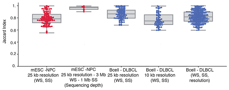
Second, Hi-C data from mESCs and NPCs at a resolution of 25 kb from the same dataset¹² were used for the reproducibility analysis of CHESS when varying two data parameters. CHESS was run using different combinations of window span (250 kb, 500 kb, 1 Mb, 2 Mb and 3 Mb) and step sizes (25 kb, 250 kb, 500 kb and 1 Mb). The Jaccard Index (JI) was calculated to obtain the overlap between the identified genomic regions. To check the reproducibility of CHESS results using different sequencing depths (percentage of reads: 80, 60, 40 and 20), we applied CHESS using 25-kb resolution, 3-Mb windows span and 500-kb step size. The data from Díaz et al.⁴⁸ were used to check how consistent was CHESS when varying three data parameters, namely different values of windows span (250 kb, 500 kb, 1 Mb, 2 Mb and 3 Mb), step sizes (25 kb, 250 kb, 500 kb and 1 Mb) and resolutions (25 kb and 10 kb). One point in the plot (Extended Data Fig. 5) corresponds to the Jaccard Index computed for a pair of CHESS runs with different combinations of parameter values. All possible pairs were compared.

Benchmark analysis

Hi-C interaction matrices at 5-kb resolution for chromosome 19 from mESCs and NPCs from Bonev et al. 2017¹² were scanned for differences using different tools. HOMER³², diffHiC³⁰ and ACCOST³¹ were run using default parameters. CHESS was run using a windows span of 1 Mb and a step size of 500 kb. All tools were run using a single CPU computational machine of the following characteristics: Intel Xeon W @ 3GHZ with 128 Gb of RAM.

In particular, CHESS was run using a windows span of 1 Mb and a step size of 500 kb. CHESS ran ~7 times faster than HOMER, ~15 times faster than diffHiC and ~320 times faster than ACCOST and had a ~4 times lower peak memory consumption than the two other tools (Extended Data Fig. 6).

To assess the similarities and differences between the three methods, we selected for each method, all bins that were involved in a significant difference between mESC and NPC contact maps. Then, the selected bins were intersected to identify those bins common to the three methods, any common bin by at least two of the three methods and, finally, any bin identified only by one of the methods (Extended Data Fig. 6). CHESS and HOMER identified about 9,000 bins with differential interactions between mESCs and NPCs while diffHiC identified about 4,000 and ACCOST about 6,000. Of the total identified differences, ~12% were identified by CHESS, HOMER, diffHiC and ACCOST. About 50% of differences were identified by CHESS and HOMER alone.

Comparison of syntenic regions between Homo sapiens and Mus musculus

We retrieved the annotations for syntenic blocks between hg19 (selected as reference) and mm10 with a resolution of 300 kb using SynBuilder³⁷. We used CHESS to compare syntenic region pairs in Hi-C matrices at 25 kb resolution for the human fibroblasts and the mouse lymphoblasts. As control, we also did comparisons between region pairs with shuffled syntenic region IDs. This was repeated 100 times. To reduce the runtime of our method, we used a randomly chosen subset of 175 syntenic regions. For the same reason, we restricted the background calculation to the query chromosome the syntenic region was located on.

Detecting structural changes between wild type and zld knockdown in Drosophila melanogaster

We obtained the locations of differential boundaries in Drosophila melanogaster and Hi-C data at 5 kb resolution for the wild type (wt), zld knockdown (kd) and water control (wc) for nuclear cycle 14 from Hug et al.⁹. From these Hi-C data we computed insulation scores as described in the same publication. We smoothed the resulting index track with a Savitzky-Golay (implemented in Scipy⁵⁹) filter (window = 29, polyorder = 2, derivative = 0). We obtained data for Zld binding ChIP-seq experiments from Blythe et al.⁷⁸.

We partitioned the D. melanogaster genome into 250 kb / 125 kb regions with a step size of 50 kb / 25 kb. We ran CHESS on the observed/expected transformed Hi-C matrices corresponding to these regions, always comparing a region in wt to the same region in wc and kd. Inside the same windows we summed the log ₁₀(q−values) for all Zld-peaks with a log ₁₀(q−value)>10 to generate the Zld binding tracks.

Using the CHESS comparisons between wt–wc and wt–kd, we defined regions with structural changes as regions located at local minima of the track with values smaller or equal to −0.1.

Differential boundaries were defined as boundaries present in wt c14 cells (calls available at https://github.com/vaquerizaslab/Hug-et-al-Cell-2017-Supp-Site) at which the difference in the log₂(insulation index) between the wt c14 and the zld knockdown was greater or equal to 0.3.

We defined differential boundaries that were closer than 125 kb / 62.5 kb to the center of a structurally changing region as captured by CHESS.

Detecting structural changes between healthy B-cells and a diffuse large B-cell lymphoma

We obtained Hi-C data from Díaz et al.⁴⁸, and processed them as described in the original publication. We partitioned the human hg19 genome into 2-Mb regions with a step size of 500 kb. We used CHESS to compare the corresponding regions in the observed/expected transformed Hi-C data from the healthy B-cells (control) and a diffuse large B-cell lymphoma (patient). To distinguish between actual structural differences and such attributable to noise we calculated a signal to noise ratio r for the differential signal of each matrix pair:

$$r=\frac{{\mu }_M}{{\sigma }^{2}M},M=M_{control}-M_{patient.}$$

This was done for a sliding window of 7 × 7 pixels on the matrix. The total signal to noise ratio was taken as the mean of all windows. Regions with a z-normalized similarity score ≤ −1.2 and a signal to noise ratio r ≥ 0.6 were labelled and accepted as changing.

Feature extraction from Capture-C data

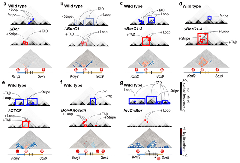
CHESS feature extraction was applied to Capture-C experiments from Despang et al.⁵⁰ (GSE125294). Interaction matrices normalized by the KR balancing method were downloaded. All the mutants were compared to the wild type. All the differential features were extracted and clustered according to their interaction pattern (see ‘The CHESS pipeline’). Three structural clusters were obtained: TAD, loop and stripe. Some examples are shown in Figure 6 and Extended Data Figure 8.

Statistics

The following statistical tests were used in this study. In Figure 3a we tested whether syntenic regions are structurally more similar than expected by chance using an one sided randomization test with 100 permutations of pairwise syntenic region assignments. For the analyses in Figures 2, 3 and Extended Data Figures 1, 4 and 7 we tested whether a particular matrix A is more similar to another particular matrix B than to other 1,000 artificially generated matrices (Fig. 2, Extended Data Figs. 1, 7) or to all other matrices along the diagonal of B’s whole chromosome matrix of the same size as A (Fig. 3, Extended Data Fig. 4). The specific details of each of these tests are described in the Online Methods sections ‘The CHESS pipeline’ and ‘Generation of synthetic Hi-C matrices’.

Extended Data

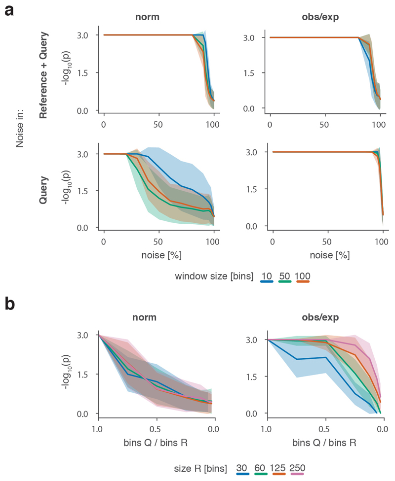
Extended Data Fig. 1. Performance analysis of the CHESS algorithm.

a, CHESS p-values in dependence of the relative noise level in synthetic matrices. Shown are the cases of equal amounts of noise in reference R and query Q (top) and different amounts of noise (bottom, noise only added to Q). Each case is examined for normalised and observed/expected (obs/exp) matrices, and different window sizes in the SSIM algorithm. b, Empirically determined CHESS p-values in dependence of the size factor between R and Q for normalised (left) and observed/expected (obs/exp) matrices (right) (details in Online Methods). a, b, Solid lines indicate the mean, shaded areas the standard deviation over 100 simulations per parameter combination.

Extended Data Fig. 2. Technical details of the SSIM algorithm applied to Hi-C matrices.

a, Schematic overview of the structural similarity algorithm (SSIM). SSIM scores are calculated on all submatrices of R / Q at a given window size (WS). The final SSIM score is the mean of all SSIM submatrix scores. b, SSIM submatrix formula. Different components are coloured: illuminance (green), structure * contrast (red). x, y refer to submatrices (at the same positions) of the two full matrices for which the SSIM average is computed (see panel a). μ indicates the mean, σ the standard deviation, c1 and c2 are small constants that are introduced only for numerical reasons. c and d, SSIM comparisons of a matrix to itself (red dots) and 1,000 random matrices of the same size (blue dots). c, SSIM component values in dependence of SSIM score for different SSIM window sizes. d, Scatterplots of ranked SSIM scores at window size 100 vs. ranked scores at smaller window sizes.

Extended Data Fig. 3. Additional analysis of the CHESS algorithm.

a, Uniform distribution of empirically determined CHESS p-values for comparisons of matrices with 100 % noise added. b, Distribution of structural similarity scores (ssim) for background and truth comparisons at 25 k/Mb and 1.5 M/Mb simulated sequencing depth. Above each: Fractional change (value at x % noise/value at 0 % noise) of the standard deviation (std) of background scores and mean of truth scores over 100 simulations per parameter combination.

Extended Data Fig. 4. CHESS is robust to changes in noise due to random ligations and sequencing depth in real Hi-C data.

a, Examples of 5 Mb matrices used in this analysis including a 5, 80 and 95 % of added noise (random ligations between pairs of loci). We tested to what extent CHESS is able to identify two matrices as being identical, after noise and sequencing depth were adjusted independently in them. Matrices are based on chromosome 19 data from Bonev et al. 2017¹². a, examples of the data with different amounts of noise. b, empirically determined p-values and z-scores of CHESS runs with different window sizes, noise levels and simulated sequencing depths (details in Online Methods). Step size and matrix resolution were both 25 kb. Lines for 2 x 10⁵ and 1 x 10⁶ overlap for runs with window sizes > 1 Mb. c, As in panel a, but comparing CHESS runs with 2.5 Mb window size on matrices binned at 25 kb and 10 kb. b, and c, solid lines indicate the mean, shaded areas the standard deviation over 1976, 2066, 2156, 2246, 2300 matrix pairs for window sizes 10 Mb, 7.5 Mb, 5 Mb, 2.5 Mb, 1 Mb, respectively.

Extended Data Fig. 5. Reproducibility of CHESS using different window (WS) and step sizes (SS), sequencing depths and resolutions.

For this analysis were tested the WS (250 kb - 3 Mb), SS (25 kb - 1 Mb), sequencing depths (percentage of reads between 20 and 80) and resolutions (10 kb and 25 kb) (details in Online Methods). X-axis labels: varied parameters in parentheses, fixed parameters before. The first two boxplots with red dots represent the Jaccard indices (JI) between CHESS results in Bonev et al. 2017¹² using different WS, SS and sequencing depths. The boxplots with blue dots correspond to the Díaz et al.⁴⁸ dataset; in this case using different WS, SS, and then between different WS, SS and resolutions. mESC mouse embryonic stem cells, NPC neural progenitor cells. Boxplot elements: centre line: median, whiskers: 1.5x interquartile range, box limits: upper-lower quartile.

Extended Data Fig. 6. CHESS benchmark against HOMER, diffHiC and ACCOST.

a, Upset plot representing the intersection size between differential interactions of CHESS, HOMER, diffHiC and ACCOST. Below, an example is shown for each intersected group. b, Computational requirements of CHESS, HOMER, diffHiC and ACCOST. The first line plot shows the CPU usage, the second the memory consumption. The vertical dashed line represents the end of the run.

Extended Data Fig. 7. CHESS performance on differently sized simulated matrices with realistic noise and sequencing depth.

Shown are empirically determined CHESS p- and z-scores (details in Online Methods) for comparisons of R with a read depth of 100 read pairs / 100 bins and a resized copy Q. Scaling factor is indicated on the x-axis. A noise level of 25 % was added to both matrices independently. Sequencing depth was adjusted to 100 k/Mb. Solid lines indicate the mean, shaded areas the standard deviation over 100 simulations per parameter combination. Colours correspond to the different sizes of R.

Extended Data Fig. 8. Feature extraction from Capture-C data.

Examples of differential feature extraction with CHESS between the wt (top contact map) and different mutants (middle contact map) in the Despang et al.⁵⁰ dataset. Lost and gained structures in the mutants are highlighted in blue and red squares, respectively. Log₂ fold-change maps are depicted below (bottom contact map) with identified features coloured according to the directionality of the change. Below each comparison, the genomic annotation is represented, highlighting the modification of each mutant. The vertical lines define the CTCF binding motifs, dashed when deleted. Red hexagons demarcate TAD boundaries. Feature extraction between wt and a, ΔBor, in which the border was deleted. b, ΔBorC1, in which the border and the first CTCF binding motif were deleted. C, ΔBorC1-2, in which the border and the two first CTCF binding motifs were deleted. d, ΔBorC1-4, in which the border and four CTCF binding motifs were deleted. e, ΔCTCF, in which the border and all the CTCF binding motifs were removed. f, Bor-KnockIn, in which the border was moved to a new location within the Sox9 locus. g, InvCΔBor, in which the Sox9 sequence was inverted and the border was removed.

Data Availability

The datasets analyzed in this study have been obtained from Gene Expression Omnibus (GEO; Rao et al., 2014: GSE63525¹⁰; Bonev et al., 2017: GSE96107¹²; Despang et al., 2019: GSE125294⁵⁰) and ArrayExpress (Hug et al., 2017: E-MTAB-4918⁹; Díaz et al., 2018: E-MTAB-5875⁴⁸).

Code Availability

The CHESS source code, as well as code for generating synthetic Hi-C matrices and running tests on them is available on GitHub: (https://github.com/vaquerizaslab/CHESS). The intervaltree and tqdm packages used internally in CHESS can be found at https://github.com/chaimleib/intervaltree and https://github.com/tqdm/tqdm, respectively.

In addition, CHESS uses internally the following published packages: FAN-C⁵⁷ (https://github.com/vaquerizaslab/fanc), Cython⁵⁸, SciPy⁵⁹, Scikit-image⁶⁰, NumPy^61,62, Pandas⁶³, Pathos⁶⁴, Pybedtools⁶⁵, Kneed⁶⁶.

References

- 1.Bonev B, Cavalli G. Organization and function of the 3D genome. Nat Rev Genet. 2016;17:661–678. doi: 10.1038/nrg.2016.112. [DOI] [PubMed] [Google Scholar]
- 2.Vietri Rudan M, et al. Comparative Hi-C Reveals that CTCF Underlies Evolution of Chromosomal Domain Architecture. Cell Reports. 2015;10:1297–1309. doi: 10.1016/j.celrep.2015.02.004. [DOI] [PMC free article] [PubMed] [Google Scholar]
- 3.Acemel RD, Maeso I, GÓmez-Skarmeta JL. Topologically associated domains: a successful scaffold for the evolution of gene regulation in animals. WIREs Developmental Biology. 2017;6:e265. doi: 10.1002/wdev.265. [DOI] [PubMed] [Google Scholar]
- 4.Lazar NH, et al. Epigenetic maintenance of topological domains in the highly rearranged gibbon genome. Genome Res. 2018 doi: 10.1101/gr.233874.117. [DOI] [PMC free article] [PubMed] [Google Scholar]
- 5.Eres IE, Luo K, Hsiao CJ, Blake LE, Gilad Y. Reorganization of 3D genome structure may contribute to gene regulatory evolution in primates. PLoS Genet. 2019;15 doi: 10.1371/journal.pgen.1008278. [DOI] [PMC free article] [PubMed] [Google Scholar]
- 6.Yang Y, Zhang Y, Ren B, Dixon JR, Ma J. Comparing 3D Genome Organization in Multiple Species Using Phylo-HMRF. Cell Systems. 2019;8:494–505.:e14. doi: 10.1016/j.cels.2019.05.011. [DOI] [PMC free article] [PubMed] [Google Scholar]
- 7.Ke Y, et al. 3D Chromatin Structures of Mature Gametes and Structural Reprogramming during Mammalian Embryogenesis. Cell. 20;170:367–381.:e20. doi: 10.1016/j.cell.2017.06.029. [DOI] [PubMed] [Google Scholar]
- 8.Du Z, et al. Allelic reprogramming of 3D chromatin architecture during early mammalian development. Nature. 2017;547:232–235. doi: 10.1038/nature23263. [DOI] [PubMed] [Google Scholar]
- 9.Hug CB, Grimaldi AG, Kruse K, Vaquerizas JM. Chromatin Architecture Emerges during Zygotic Genome Activation Independent of Transcription. Cell. 19;169:216–228.:e19. doi: 10.1016/j.cell.2017.03.024. [DOI] [PubMed] [Google Scholar]
- 10.Rao SSP, et al. A 3D map of the human genome at kilobase resolution reveals principles of chromatin looping. Cell. 2014;159:1665–1680. doi: 10.1016/j.cell.2014.11.021. [DOI] [PMC free article] [PubMed] [Google Scholar]
- 11.Dixon JR, et al. Chromatin architecture reorganization during stem cell differentiation. Nature. 2015;518:331–336. doi: 10.1038/nature14222. [DOI] [PMC free article] [PubMed] [Google Scholar]
- 12.Bonev B, et al. Multiscale 3D Genome Rewiring during Mouse Neural Development. Cell. 2017;171:557–572.:e24. doi: 10.1016/j.cell.2017.09.043. [DOI] [PMC free article] [PubMed] [Google Scholar]
- 13.Nagano T, et al. Cell-cycle dynamics of chromosomal organization at single-cell resolution. Nature. 2017;547:61–67. doi: 10.1038/nature23001. [DOI] [PMC free article] [PubMed] [Google Scholar]
- 14.Gibcus JH, et al. A pathway for mitotic chromosome formation. Science. 2018;359 doi: 10.1126/science.aao6135. [DOI] [PMC free article] [PubMed] [Google Scholar]
- 15.Spielmann M, LupiÃńez DG, Mundlos S. Structural variation in the 3D genome. Nat Rev Genet. 2018;19:453–467. doi: 10.1038/s41576-018-0007-0. [DOI] [PubMed] [Google Scholar]
- 16.Krijger PHL, de Laat W. Regulation of disease-associated gene expression in the 3D genome. Nat Rev Mol Cell Biol. 2016;17:771–782. doi: 10.1038/nrm.2016.138. [DOI] [PubMed] [Google Scholar]
- 17.Darrow EM, et al. Deletion of DXZ4 on the human inactive X chromosome alters higher-order genome architecture. PNAS. 2016;113:E4504–E4512. doi: 10.1073/pnas.1609643113. [DOI] [PMC free article] [PubMed] [Google Scholar]
- 18.Dixon JR, et al. Topological domains in mammalian genomes identified by analysis of chromatin interactions. Nature. 2012;485:376–380. doi: 10.1038/nature11082. [DOI] [PMC free article] [PubMed] [Google Scholar]
- 19.Crane E, et al. Condensin-driven remodelling of X chromosome topology during dosage compensation. Nature. 2015;523:240–244. doi: 10.1038/nature14450. [DOI] [PMC free article] [PubMed] [Google Scholar]
- 20.Yang T, et al. HiCRep: assessing the reproducibility of Hi-C data using a stratum-adjusted correlation coefficient. Genome Res. 2017;27:1939–1949. doi: 10.1101/gr.220640.117. [DOI] [PMC free article] [PubMed] [Google Scholar]
- 21.Sauria ME, Taylor J. QuASAR: Quality Assessment of Spatial Arrangement Reproducibility in Hi-C Data. bioRxiv. 2017:204438. doi: 10.1101/204438. [DOI] [Google Scholar]
- 22.Ursu O, et al. GenomeDISCO: a concordance score for chromosome conformation capture experiments using random walks on contact map graphs. Bioinformatics. 2018;34:2701–2707. doi: 10.1093/bioinformatics/bty164. [DOI] [PMC free article] [PubMed] [Google Scholar]
- 23.Yan K-K, Yardımcı GG, Yan C, Noble WS, Gerstein M. HiC-spector: a matrix library for spectral and reproducibility analysis of Hi-C contact maps. Bioinformatics. 2017;33:2199–2201. doi: 10.1093/bioinformatics/btx152. [DOI] [PMC free article] [PubMed] [Google Scholar]
- 24.Shavit Y, LiÓ P. Combining a wavelet change point and the Bayes factor for analysing chromosomal interaction data. Mol Biosyst. 2014;10:1576–1585. doi: 10.1039/c4mb00142g. [DOI] [PubMed] [Google Scholar]
- 25.Huynh L, Hormozdiari F. Contribution of structural variation to genome structure: TAD fusion discovery and ranking. bioRxiv. 2018:279356. doi: 10.1101/279356. [DOI] [PMC free article] [PubMed] [Google Scholar]
- 26.Paulsen J, et al. HiBrowse: multi-purpose statistical analysis of genome-wide chromatin 3D organization. Bioinformatics. 2014;30:1620–1622. doi: 10.1093/bioinformatics/btu082. [DOI] [PMC free article] [PubMed] [Google Scholar]
- 27.Lareau CA, Aryee MJ. diffloop: a computational framework for identifying and analyzing differential DNA loops from sequencing data. Bioinformatics. 2018;34:672–674. doi: 10.1093/bioinformatics/btx623. [DOI] [PMC free article] [PubMed] [Google Scholar]
- 28.Djekidel MN, Chen Y, Zhang MQ. FIND: difFerential chromatin INteractions Detection using a spatial Poisson process. Genome Res. 2018;28:412–422. doi: 10.1101/gr.212241.116. [DOI] [PMC free article] [PubMed] [Google Scholar]
- 29.Stansfield JC, Cresswell KG, Vladimirov VI, Dozmorov MG. HiCcompare: an R-package for joint normalization and comparison of HI-C datasets. BMC Bioinformatics. 2018;19 doi: 10.1186/s12859-018-2288-x. [DOI] [PMC free article] [PubMed] [Google Scholar]
- 30.Lun ATL, Smyth GK. diffHic: a Bioconductor package to detect differential genomic interactions in Hi-C data. BMC Bioinformatics. 2015;16:258. doi: 10.1186/s12859-015-0683-0. [DOI] [PMC free article] [PubMed] [Google Scholar]
- 31.Cook KB, Hristov BH, Le Roch KG, Vert JP, Noble WS. Measuring significant changes in chromatin conformation with ACCOST. Nucleic Acids Res. 2020;48:2303–2311. doi: 10.1093/nar/gkaa069. [DOI] [PMC free article] [PubMed] [Google Scholar]
- 32.Heinz S, et al. Simple Combinations of Lineage-Determining Transcription Factors Prime cis-Regulatory Elements Required for Macrophage and B Cell Identities. Molecular Cell. 2010;38:576–589. doi: 10.1016/j.molcel.2010.05.004. [DOI] [PMC free article] [PubMed] [Google Scholar]
- 33.Wang Z, Bovik AC, Sheikh HR, Simoncelli EP. Image Quality Assessment: From Error Visibility to Structural Similarity. IEEE Transactions on Image Processing. 2004;13:600–612. doi: 10.1109/tip.2003.819861. [DOI] [PubMed] [Google Scholar]
- 34.Wang Zhou, Bovik AC. A universal image quality index. IEEE Signal Processing Letters. 2002;9:81–84. [Google Scholar]
- 35.Lieberman-Aiden E, et al. Comprehensive mapping of long-range interactions reveals folding principles of the human genome. Science. 2009;326:289–293. doi: 10.1126/science.1181369. [DOI] [PMC free article] [PubMed] [Google Scholar]
- 36.Harmston N, et al. Topologically associating domains are ancient features that coincide with Metazoan clusters of extreme noncoding conservation. Nat Commun. 2017;8:1–13. doi: 10.1038/s41467-017-00524-5. [DOI] [PMC free article] [PubMed] [Google Scholar]
- 37.Lee J, et al. Synteny Portal: a web-based application portal for synteny block analysis. Nucleic Acids Res. 2016;44:W35–40. doi: 10.1093/nar/gkw310. [DOI] [PMC free article] [PubMed] [Google Scholar]
- 38.Schwarzer W, et al. Two independent modes of chromatin organization revealed by cohesin removal. Nature. 2017;551:51–56. doi: 10.1038/nature24281. [DOI] [PMC free article] [PubMed] [Google Scholar]
- 39.Nora EP, et al. Targeted Degradation of CTCF Decouples Local Insulation of Chromosome Domains from Genomic Compartmentalization. Cell. 2017;169:930–944.:e22. doi: 10.1016/j.cell.2017.05.004. [DOI] [PMC free article] [PubMed] [Google Scholar]
- 40.Haarhuis JHI, et al. The Cohesin Release Factor WAPL Restricts Chromatin Loop Extension. Cell. 2017;169:693–707.:e14. doi: 10.1016/j.cell.2017.04.013. [DOI] [PMC free article] [PubMed] [Google Scholar]
- 41.Rao SSP, et al. Cohesin Loss Eliminates All Loop Domains. Cell. 24;171:305–320.:e24. doi: 10.1016/j.cell.2017.09.026. [DOI] [PMC free article] [PubMed] [Google Scholar]
- 42.Wutz G, et al. Topologically associating domains and chromatin loops depend on cohesin and are regulated by CTCF, WAPL, and PDS5 proteins. EMBO J. 2017;36:3573–3599. doi: 10.15252/embj.201798004. [DOI] [PMC free article] [PubMed] [Google Scholar]
- 43.Gassler J, et al. A mechanism of cohesin-dependent loop extrusion organizes zygotic genome architecture. EMBO J. 2017;36:3600–3618. doi: 10.15252/embj.201798083. [DOI] [PMC free article] [PubMed] [Google Scholar]
- 44.LupiÃńez DG, et al. Disruptions of topological chromatin domains cause pathogenic rewiring of gene-enhancer interactions. Cell. 2015;161:1012–1025. doi: 10.1016/j.cell.2015.04.004. [DOI] [PMC free article] [PubMed] [Google Scholar]
- 45.Franke M, et al. Formation of new chromatin domains determines pathogenicity of genomic duplications. Nature. 2016;538:265–269. doi: 10.1038/nature19800. [DOI] [PubMed] [Google Scholar]
- 46.Flavahan WA, et al. Insulator dysfunction and oncogene activation in IDH mutant gliomas. Nature. 2016;529:110–114. doi: 10.1038/nature16490. [DOI] [PMC free article] [PubMed] [Google Scholar]
- 47.Hnisz D, et al. Activation of proto-oncogenes by disruption of chromosome neighborhoods. Science. 2016;351:1454–1458. doi: 10.1126/science.aad9024. [DOI] [PMC free article] [PubMed] [Google Scholar]
- 48.Daíz N, et al. Chromatin conformation analysis of primary patient tissue using a low input Hi-C method. Nat Commun. 2018;9:1–13. doi: 10.1038/s41467-018-06961-0. [DOI] [PMC free article] [PubMed] [Google Scholar]
- 49.Hughes JR, et al. Analysis of hundreds of cis-regulatory landscapes at high resolution in a single, high-throughput experiment. Nat Genet. 2014;46:205–212. doi: 10.1038/ng.2871. [DOI] [PubMed] [Google Scholar]
- 50.Despang A, et al. Functional dissection of the Sox9-Kcnj2 locus identifies nonessential and instructive roles of TAD architecture. Nat Genet. 2019;51:1263–1271. doi: 10.1038/s41588-019-0466-z. [DOI] [PubMed] [Google Scholar]
- 51.Kalhor R, Tjong H, Jayathilaka N, Alber F, Chen L. Genome architectures revealed by tethered chromosome conformation capture and population-based modeling. Nat Biotechnol. 2011;30:90–98. doi: 10.1038/nbt.2057. [DOI] [PMC free article] [PubMed] [Google Scholar]
- 52.Lin D, et al. Digestion-ligation-only Hi-C is an efficient and cost-effective method for chromosome conformation capture. Nat Genet. 2018;50:754–763. doi: 10.1038/s41588-018-0111-2. [DOI] [PubMed] [Google Scholar]
- 53.Beagrie RA, et al. Complex multi-enhancer contacts captured by genome architecture mapping. Nature. 2017;543:519–524. doi: 10.1038/nature21411. [DOI] [PMC free article] [PubMed] [Google Scholar]
- 54.Cardozo Gizzi AM, et al. Microscopy-Based Chromosome Conformation Capture Enables Simultaneous Visualization of Genome Organization and Transcription in Intact Organisms. Mol Cell. 2019;74:212–222.:e5. doi: 10.1016/j.molcel.2019.01.011. [DOI] [PubMed] [Google Scholar]
- 55.Sampat MP, Wang Z, Gupta S, Bovik AC, Markey MK. Complex Wavelet Structural Similarity: A New Image Similarity Index. IEEE Transactions on Image Processing. 2009;18:2385–2401. doi: 10.1109/TIP.2009.2025923. [DOI] [PubMed] [Google Scholar]
- 56.Homola T, Dohnal V, Zezula P. Searching for Sub-images Using Sequence Alignment. Proceedings of the 2011 IEEE International Symposium on Multimedia; IEEE Computer Society. 2011. pp. 61–68. [DOI] [Google Scholar]
- 57.Kruse K, Hug CB, Vaquerizas JM. FAN-C: A Feature-rich Framework for the Analysis and Visualisation of C data. bioRxiv. 2020:2020.02.03.932517. doi: 10.1101/2020.02.03.932517. [DOI] [PMC free article] [PubMed] [Google Scholar]
- 58.Behnel S, et al. Cython: The Best of Both Worlds. Computing in Science & Engineering. 2011;13:31–39. [Google Scholar]
- 59.Virtanen P, et al. SciPy 1.0: fundamental algorithms for scientific computing in Python. Nat Methods. 2020;17:261–272. doi: 10.1038/s41592-019-0686-2. [DOI] [PMC free article] [PubMed] [Google Scholar]
- 60.van der Walt S, et al. scikit-image: image processing in Python. PeerJ. 2014;2:e453. doi: 10.7717/peerj.453. [DOI] [PMC free article] [PubMed] [Google Scholar]
- 61.Oliphant TE. A guide to NumPy. Vol. 1 Trelgol Publishing USA; 2006. [Google Scholar]
- 62.van der Walt S, Colbert SC, Varoquaux G. The NumPy Array: A Structure for Efficient Numerical Computation. Computing in Science Engineering. 2011;13:22–30. [Google Scholar]
- 63.McKinney W. Data Structures for Statistical Computing in Python. Python in Science Conference; 2010. pp. 56–61. [DOI] [Google Scholar]
- 64.McKerns MM, Strand L, Sullivan T, Fang A, Aivazis MAG. Building a Framework for Predictive Science. arXiv. 2012:1202.1056. [cs] [Google Scholar]
- 65.Dale RK, Pedersen BS, Quinlan AR. Pybedtools: a flexible Python library for manipulating genomic datasets and annotations. Bioinformatics. 2011;27:3423–3424. doi: 10.1093/bioinformatics/btr539. [DOI] [PMC free article] [PubMed] [Google Scholar]
- 66.Satopaa V, Albrecht J, Irwin D, Raghavan B. Finding a ‛Kneedle“ in a Haystack: Detecting Knee Points in System Behavior. 31st International Conference on Distributed Computing Systems Workshops; 2011. pp. 166–171. [DOI] [Google Scholar]
- 67.Imakaev M, et al. Iterative correction of Hi-C data reveals hallmarks of chromosome organization. Nat Methods. 2012;9:999–1003. doi: 10.1038/nmeth.2148. [DOI] [PMC free article] [PubMed] [Google Scholar]
- 68.Knight PA, Ruiz D. A fast algorithm for matrix balancing. IMA J Numer Anal. 2013;33:1029–1047. [Google Scholar]
- 69.Behara KNS, Bhaskar A, Chung E. Geographical window based structural similarity index for OD matrices comparison. 2020 https://eprints.qut.edu.au/133466/
- 70.Djukic T, Hoogendoorn S, Van Lint H. Reliability Assessment of Dynamic OD Estimation Methods Based on Structural Similarity Index. Transportation Research Board 92nd Annual MeetingTransportation Research Board; 2013. [Google Scholar]
- 71.Breakey D, Meskell C. Comparison of metrics for the evaluation of similarity in acoustic pressure signals. Journal of Sound and Vibration. 2013;332:3605–3609. [Google Scholar]
- 72.Hines A, Harte N. Speech intelligibility prediction using a Neurogram Similarity Index Measure. Speech Communication. 2012;54:306–320. [Google Scholar]
- 73.Tomasi C, Manduchi R. Bilateral filtering for gray and color images. Sixth International Conference on Computer Vision; IEEE; 1998. pp. 839–846. Cat. No.98CH36271) [DOI] [Google Scholar]
- 74.Otsu N. A Threshold Selection Method from Gray-Level Histograms. IEEE Transactions on Systems, Man, and Cybernetics. 1979;9:62–66. [Google Scholar]
- 75.Sexton T, et al. Three-Dimensional Folding and Functional Organization Principles of the Drosophila Genome. Cell. 2012;148:458–472. doi: 10.1016/j.cell.2012.01.010. [DOI] [PubMed] [Google Scholar]
- 76.Cock PJA, et al. Biopython: freely available Python tools for computational molecular biology and bioinformatics. Bioinformatics. 2009;25:1422–1423. doi: 10.1093/bioinformatics/btp163. [DOI] [PMC free article] [PubMed] [Google Scholar]
- 77.Cournac A, Marie-Nelly H, Marbouty M, Koszul R, Mozziconacci J. Normalization of a chromosomal contact map. BMC Genomics. 2012;13:436. doi: 10.1186/1471-2164-13-436. [DOI] [PMC free article] [PubMed] [Google Scholar]
- 78.Blythe SA, Wieschaus EF. Zygotic Genome Activation Triggers the DNA Replication Checkpoint at the Midblastula Transition. Cell. 2015;160:1169–1181. doi: 10.1016/j.cell.2015.01.050. [DOI] [PMC free article] [PubMed] [Google Scholar]
Associated Data
This section collects any data citations, data availability statements, or supplementary materials included in this article.
Supplementary Materials
Data Availability Statement