Nearest neighbors reveal fast and slow components of motor learning

Abstract

Changes in behavior, due to environmental influences, development, and learning^1–5, are commonly quantified based on a few hand-picked, domain-specific, features^2–4,6,7 (e.g. the average pitch of acoustic vocalizations³) and assuming discrete classes of behaviors (e.g. distinct vocal syllables)^2,3,8–10. Such methods generalize poorly across different behaviors and model systems and may miss important components of change. Here we present a more general account of behavioral change based on nearest-neighbor statistics^11–13 and apply it to song development in a songbird, the zebra finch³. First, we introduce “repertoire dating”, whereby each rendition of a behavior (e.g. each vocalization) is assigned a repertoire time, reflecting when similar renditions were typical in the behavioral repertoire. Repertoire time (rT) isolates the components of vocal variability congruent with the long-term changes due to vocal learning and development and stratifies the behavioral repertoire into regressions (rT < true production time, t), anticipations (rT > t), and typical renditions (rT ≈ t). Second, we obtain a holistic, yet low-dimensional¹⁴, description of vocal change in terms of a stratified “behavioral trajectory”, revealing multiple, previously unrecognized, components of behavioral change on fast and slow timescales, as well as distinct patterns of overnight consolidation^1,2,4,15,16. Diurnal changes in regressions undergo only weak consolidation, whereas anticipations and typical renditions consolidate fully. Because of its generality, our non-parametric description of how behavior evolves relative to itself, rather than relative to a potentially arbitrary, experimenter-defined, goal^2,3,15,17 appears well-suited to compare learning and change across behaviors and species^18,19, as well as biological and artificial systems⁵.

Zebra finches acquire complex, stereotyped, vocalizations through a months-long process of sensory-motor learning^3,20–22. We obtained dense audio recordings between 35-123 days post hatch (dph) in 5 male birds (73.4±18.6 consecutive days, mean±STD). Birds were isolated from other males after birth and, on average, live-tutored between dph46 and 63 (Extended Data Fig. 1a). Band passed (0.35-8kHz) audio recordings were segmented into individual vocal renditions, and represented as song spectrogram segments (Fig. 1a, 563, 124-1, 203, 647 renditions per bird). Noise and isolated calls were excluded from the analyses. During development, syllable order, i.e. syntax, and the spectral structure of syllables evolve³. These two aspects of vocal learning may be mediated by largely independent mechanisms with distinct anatomical substrates²³. Here we focus on characterizing the development of spectral structure.

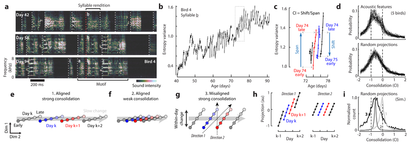
Figure 1. Fast and slow change in developing zebra finch vocalizations.

(a) Vocalizations at three developmental stages. Dotted lines indicate syllable onsets. Crystalized song syllables (middle and bottom) fall into discrete categories (syllables i, a, b, c) and form a stereotyped motif, typically resembling the tutor song.

(b) Time course of the acoustic feature entropy variance for syllable b.

(c) Cutout from (b) with within-day span (early to late, day k) and overnight shift (late day k to early day k+1). Consolidation index (CI)≈ -0.75.

(d) Histograms of CIs over pairs of consecutive days, syllables and birds, for 32 acoustic features (top) and 32 random spectral projections (bottom).

(e-g) Three scenarios of slow developmental change (gray arrows; dim 2) and fast within-day change in vocalizations. Each point represents the distribution of vocalizations from a given time and day. A larger distance between points indicates more dissimilar distributions. Different directions correspond to distinct song features.

(h) Linear projections of the points in (g) onto two example directions (g, dotted lines) for the misaligned, strong-consolidation scenario. Consolidation strength varies across directions.

(i) Consolidation indices over 10,000 random projections simulated from the three scenarios (labels 1, 2, and 3; see e-g).

Behavioral change in single features

Vocal development is often characterized by considering change in acoustic features such as pitch, frequency modulation³, or entropy variance^2,15 (Fig. 1b). Such characterizations readily reveal multiple timescales of behavioral change—individual features can vary consistently within a day; can display overnight discontinuities; and can show drifts over the duration of weeks or months (Fig. 1b,c).

We summarize the relation between change at these different timescales through a consolidation index (Fig. 1c, CI), measuring whether within-day change in a feature (Fig. 1c, span) is maintained or lost overnight (Fig. 1c, shift). Weak consolidation^2,15 corresponds to a CI close to -1 (no consolidation: shift = -span), strong consolidation^4,16 to a CI close to 0 (perfect consolidation: shift = 0 days), and offline learning^4,24,25 to a CI larger than 0. Across 32 commonly used acoustic features, CIs are mostly negative, indicating weak consolidation (Fig. 1d, top, median: -0.67). This finding holds even for random spectral features (Fig. 1d, bottom, median: -0.64) and is consistent with past accounts of song-development in zebra finches^2,15.

Individual features, however, may provide an incomplete account of change in a complex behavior such as song vocalizations. To illustrate this point, we consider three simple scenarios. In the first two (Fig. 1e,f), the change in behavior occurring within any given day largely mirrors, on a faster timescale, the slow change occurring over the course of many days or weeks. In the third scenario (Fig. 1g), within-day change is partly “misaligned” with slow change, i.e. it involves behavioral features that do not consistently change on slower timescales. Within-day change could reflect metabolic, neural, or other changes that are not necessarily congruent with longer-term learning or development; the slow change reflects long-term modifications in behavior typically equated with learning and development. We abstractly refer to these slow components as the direction of slow change (DiSC).

Critically, simulations of these scenarios show that negative CIs for single features can result from very different time courses of development (Fig. 1h, i). Negative CIs occur both when within-day and slow changes are closely aligned but daily gains along the DiSC are mostly lost overnight (Fig. 1f, weak consolidation), as well as when diurnal gains along the DiSC are perfectly consolidated, but within-day change is substantially misaligned with slow change (Fig. 1g). The broad distributions of indices observed during song development (Fig. 1d, top), which also include strongly positive indices, seem more consistent with the misaligned scenario (Fig. 1i, histogram 3).

Nearest-neighbor measures of change

We developed a general characterization of high-dimensional behavioral change, based on nearest-neighbor statistics^12,13that can distinguish between the scenarios in Fig. 1e-g. We initially analyze song-spectrogram segments of fixed duration aligned to syllable onset (Fig. 1a) but later extend our analysis to alternative parameterizations of vocalizations. Vocal renditions are represented as vectors x_i ∈ ℝ^d (i indexes renditions), each associated with a production time, t_i ∈ ℝ (e.g. the bird’s age when singing x_i). The K-neighborhood of rendition x_i is given by those K renditions (among the set of all renditions) that are closest to x_i based on some metric (e.g. Euclidean distance). For small enough K, different syllable types do not mix within a neighborhood (Extended Data Fig. 1e, Fig. 3a) and neighborhood statistics are largely independent of cluster boundaries, obviating the need for clustering renditions into syllables.

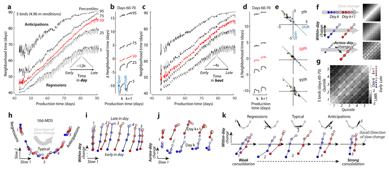
Figure 3. Multiple components of behavioral change during sensory-motor learning.

(a) Average repertoire dating percentiles (5 birds) chart within and across-day changes along the direction of slow change (DiSC). For each production day and period, 5 percentiles of the pooled neighborhood times (Fig. 2c) are arranged vertically (lines).

(b) Average of (a) across days 60-70, expressed relative to the average 50^th percentile.

(c) Within-bout changes. Like (a), but based on production day and period in a singing bout.

(d) Like (b), averaged from (c).

(e) Span and shift for the 5^th, 50^th, and 95^th percentile (blue arrows in (b), analogous to Fig. 1c) averaged over days 50-80, separately for syllables (points) and birds (colors). Black: median and 95% bootstrapped confidence intervals over all points.

(f) Simulated stratified mixing matrices (sMM, right) for three models (left) of the alignment of within-day and across-day change with the DiSC.

(g) Average sMM (5 birds, days 60-70).

(h-j) Stratified behavioral trajectory based on (g). Different 2-d projections reveal the DiSC (h), as well as within-day (i) and across-day (j) change not aligned with the DiSC (labels 1-5: strata). Full 10-d trajectories faithfully reproduce sMM structure (MDS stress = 0.016); the depicted 4-d subspace (h-j) captures 81% of the 10-d variance.

(k) Separate projections for each stratum onto the local DiSC (inset, black arrows; points represent strata from (h)).

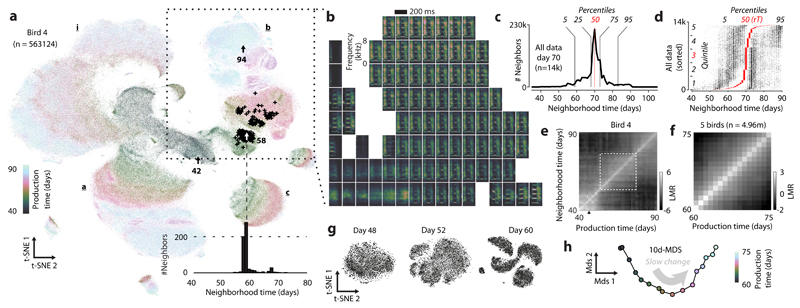
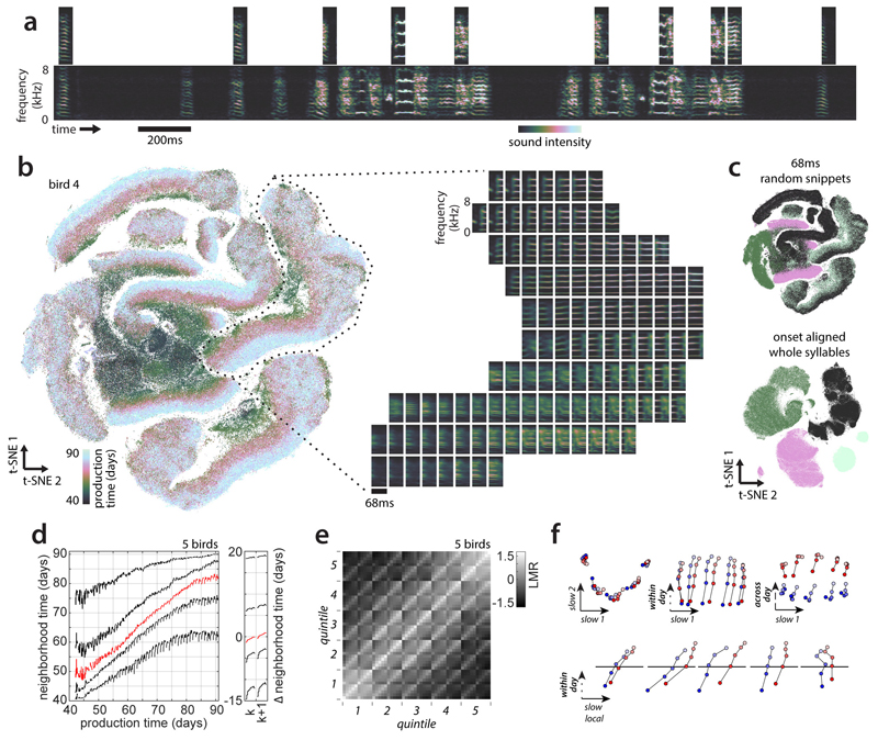
We visualize all vocalizations produced by a bird throughout development with Barnes-Hut-t-SNE¹¹ (which predominantly preserves local neighborhoods¹¹). Each point in the embedding corresponds to a spectrogram segment x_i (Fig. 1a). Different locations correspond to different vocalization types (Fig. 2b, Extended Data Fig. 2a,d). The embedding suggests that vocalizations change from undifferentiated subsong^3,21 (Fig. 2a, middle) to clearly differentiated syllables falling into at least four categories (Fig. 2a, syllables a, b, c and introductory note i; same labels as in Fig. 1a). The emergence of clustered syllables from un-clustered subsong is confirmed by standard clustering approaches (Fig. 2g, Extended Data Fig. 1). Notably, the embedding does not preserve all local structure in the data, as nearest neighbors in the embedding space are not necessarily nearest neighbors in the high dimensional data space (Fig. 2a;black crosses: high-d neighbors). We therefore quantify behavioral change directly on the high-dimensional databy analyzing the composition of high dimensional neighborhoods^12,13 (Extended Data Fig. 2).

Figure 2. Neighborhood mixing and repertoire dating.

(a) t-SNE of all vocalizations from the bird in Fig. 1a. Each point is a syllable rendition. Clusters (syllables i, a, b, c; labels) emerge during development. Arrows: renditions of syllable b from Fig. 1a. Crosses: the 600 nearest neighbors of the rendition from day 58.

(b) Average spectrograms for different locations in the t-SNE in (a). (Inset) Histogram of production times (“neighborhood times”) over the 600 nearest neighbors in (a).

(c) Pooled neighborhood times for day 70. Percentiles (vertical lines) quantify the extent of the behavioral repertoire on day 70.

(d) Percentiles (5^th, 50^th, 95^th) of neighborhood times for day 70 (each row represents a rendition). Rows are sorted by the 50^th percentile (“repertoire time”, rT, red dots). Left and right dots mark the 5^th and 95^thpercentile. A random horizontal shift was added to each dot for visualization.

(e) Mixing-matrix for all data points depicted in (a). Each column of the matrix represents a histogram of production times, pooled over all neighborhoods of points within a day (horizontal axis), normalized by a shuffling null-hypothesis (LMR: base 2 logarithm of mixing ratio). Black arrow: first day of tutoring.

(f) Average mixing-matrix over 5 birds (days 60-75).

(g) Single-day t-SNE, for 3 days (bird 4), illustrating the gradual emergence of clusters.

(h) Behavioral trajectory based on (f), 10-d multi-dimensional scaling. Each point corresponds to a day. The 2 dimensions capturing most variance in the trajectory are shown.

For each datapoint, we refer to the production times of all data points in its K-neighborhood as the “neighborhood production times” (or “neighborhood times”; Fig. 2a, inset). We summarize the neighborhood times of many data points (Fig. 2d) through “pooled neighborhood times” (Fig. 2c) and the “neighborhood mixing-matrix” (Fig 2e; Extended Data Fig. 3d; Extended Data Fig. 2). Each value in the mixing matrix represents the similarity between behaviors from two production periods. Deviations from zero indicate that behaviors from the corresponding production periodsare more (> 0) or less (< 0) similar (i.e. mixed at the level of K-neighborhoods) than expected from a shuffling null-hypothesis.

We use multi-dimensional scaling¹⁴to represent the similarity between behaviors from different production times as a “behavioral trajectory” (Fig. 2h). Each point on the trajectory represents the distribution of all vocalizations produced on a given day. Pairwise distances between points represent the dissimilarity between distributions (Extended Data Fig. 2). Here we focus on a16-day-phase of gradual change midway through development (Fig. 2f). During this phase, the behavioral trajectory is structured differently on fast and slow timescales (Extended Data Fig. 3f-h). The 2d-projection of the trajectory that explains maximal variance mainly reflects the direction of slow change (DiSC, Fig. 2h; Fig 1e-g).

The behavioral trajectory summarizes the progressive differentiation of vocalizations into distinct syllables, as well as simultaneous, continuous, change in many spectral features of individual syllables (Extended Data Fig. 7). Notably, change is characterized through the behavioral trajectory by comparing the bird’s song to itself across time, rather than to a tutor song. Thus the behavioral trajectory may also reflect innate song priors that can result in crystallized song deviating from the tutor song²⁶ and additional change due to other developmental processes²⁷.

Repertoire extent and consolidation

t-SNE suggests that renditions from nearby days overlap considerably, whereby changes occurring within a day partly mimic the slow change across days (Extended Data Fig. 2b,c). We quantify this apparent spread along the DiSC, reflecting different degrees of behavioral “maturity”, through neighborhood times (Fig. 2d). We refer to behavioral renditions that predominantly have neighbors produced in the future as “anticipations” and to renditions that predominantly have neighbors that were produced in the past as “regressions” (Extended Data Fig. 3b). By contrast, renditions that are “typical” for a given developmental stage mostly have neighbors produced on the same or nearby days. We denote the median neighborhood time as the “repertoire time” (rT) of a rendition. The repertoire time effectively places each rendition along the DiSC (Fig. 2d, horizonal axis), i.e. dates it with respect to the progression of vocal development (“repertoire dating”). Abroad distribution of repertoire times across all renditions in a day (Fig. 2d) suggests considerable behavioral variability along the DiSC—the most extreme regressions are backdated more than 10 days into the past, and the most extreme anticipations are postdated more than 10 days into the future (Fig. 2d, rT).

To quantify behavioral change on the time scale of hours, we subdivide each day into 10 consecutive periods, and compute pooled neighborhood times separately for each period. The percentiles of the pooled neighborhood times chart the evolution of behavior within and across days throughout development (Fig. 3a). Each repertoire dating percentile is akin to a learning curve for a part of the behavioral repertoire (e.g. typical renditions, 50^th percentile; extreme anticipations, 95^th percentile). The evolution of each percentile captures the progress along the DiSC (Fig. 3a, vertical axis) over time (Fig. 3a, horizontal axis). We validated this characterization of behavioral change on simulated behavior mimicking vocal development (Extended Data Fig. 4a-d).

The repertoire-dating percentiles reveal that typical renditions move gradually along the DiSC throughout the day and changes along the DiSC acquired during the day are, on average, fully consolidated overnight (Fig. 3a,b; red). Anticipations undergo a similar or smaller degree of within-day-change (Fig. 3a, b; 75^th and 95^th percentiles) whereas regressions move by a larger distance within each day, but this change is only weakly consolidated overnight (Fig. 3a,b; 5^th and 25^th percentiles; Fig 3e). The most “immature” renditions thus improve markedly throughout a day, more than typical renditions or anticipations, but these improvements are mostly lost overnight. This pattern of change seems characteristic of development, as it is absent in adults (Extended Data Fig. 6).

Movement along the DiSC also occurs on faster timescales than hours, namely within bouts of singing, i.e. groups of vocalizations preceded and followed by a pause (average bout duration: 3.81±0.83s across birds). We subdivide each bout into 10 consecutive periods, compute pooled neighborhood times for each period (over all bouts in a day), and track change through the corresponding percentiles (Fig. 3c,d). Within bouts, large changes along the DiSC occur at the regressive tail of the behavioral repertoire—vocalizations are most regressive at the onset and offset of bouts (Fig. 3c,d; 5^th percentile). Similar, albeit weaker, changes occur for typical renditions (Fig. 3c,d; red). The same apparent changes in song maturity are observed when short and long bouts (durations 2.30±0.54s vs. 6.28±1.73s) are considered separately. Song maturity thus decreases at the end of a bout, not after a fixed time into the bout (Extended Data Fig. 5a-c).

Misaligned behavioral components

The repertoire time reveals within-day and within-bout changes that mirror, on a faster timescale, changes occurring also over many days (see Methods). As above (Fig. 1), we refer to such components of change as being aligned with the DiSC, and to components that are not reflected in the repertoire time as being misaligned.

We identify both aligned and misaligned components of change through the “stratified mixing matrix”, which combines a neighborhood mixing-matrix (e.g. Fig. 2f) with repertoire dating. Each day’s behavioral repertoire is binned into 5 consecutive production periods. Within each period, the behavioral repertoire is subdivided into 5 strata, based on repertoire time (Fig. 2e, quintiles). All renditions from a day thus fall into 5x5=25 bins. The stratified mixing matrix measures similarity between 50 bins combining data from two adjacent days (Fig. 3g). We compare the measured stratified mixing matrix with simulations differing with respect to how within-day change and change across adjacent days align with the DiSC (Fig. 3f; Extended Data Fig. 4e-j). In model 1development is “1-dimensional”, i.e. aligned with the DiSC (Fig. 3f, top; similar to Fig. 1e). In model 2, within-day change involves a component not aligned with the DiSC (Fig. 3f, middle; similar to Fig. 1g). In model 3, adjacent days are separated not only along the DiSC, but also along a direction orthogonal to both the DiSC and the direction of within day change (Fig. 3f, bottom, across-day change). Prominent “stripes” along every other diagonal in the measured mixing matrix (Fig. 3g) indicate a larger similarity between renditions from the same day than between renditions from adjacent days, as predicted by model 3, suggesting that several misaligned components contribute to change at fast timescales.

Based on the stratified mixing-matrix, we infer stratified behavioral trajectories. The 2d-projection capturing most of the variance due to strata (Fig. 3h) resembles Fig. 2 hand reflects the DiSC. Consistent with repertoire-dating, behavioral change along the DiSC between adjacent days (Fig. 3h, blue vs. red for each stratum) is small compared to the spread of one day’s behavior along the DiSC (e.g. blue points, strata 1-5). For each stratum, however, much of the change occurring within a day is misaligned with the DiSC (Fig. 3i,k; early vs. late separated along orthogonal dimension of within-day change). Yet another misaligned component is necessary to appropriately capture change across adjacent days (Fig. 3j). These properties of aligned and misaligned components are replicated by a linear analysis based on spectral features chosen to capture change at specific timescales (Extended Data Fig. 7, 8) and are robust to how song is parameterized and segmented, and to how nearest neighbors are defined (Extended Data Fig. 9, 10).

Discussion

Our analysis of high-dimensional vocalizations reveals that the developmental trajectory does not merely reflect an underlying one-dimensional process. Single behavioral features in isolation therefore provide an incomplete account of behavioral change during development and learning. The weak consolidation observed here (Fig. 1d) and elsewhere^2,15 at the level of single features appears to reflect prominent misaligned components of within-day change rather than weak consolidation along the DiSC (Fig. 1h). Strong overnight consolidation along the DiSC across much of the behavioral repertoire (Fig. 3a,b) seems consistent with consolidation patterns observed for skilled motor learning in humans^24,25,28 and of motor adaptation in humans^1,19 and birds⁴.

Our characterization of behavior based on nearest-neighbor statistics can be applied when no accurate parametric model of the behavior is known, as currently is the case for most natural, complex behaviors. The approach is largely complementary to methods that rely on clustering behavior into distinct categories^2,3,10,29. Foregoing an explicit clustering of the data can be advantageous since assuming the existence of clusters can be an unwarranted approximation³⁰; may impede the characterization of behavior that appears not clustered (such as juvenile zebra finch song; Extended Data Fig. 1);and determining correct cluster boundaries is in general an ill-defined problem³⁰. Importantly, our analyses require only an indicator function that selects nearest neighbors (here based on a “locally meaningful” distance metric), a much weaker requirement than a globally valid distance metric or the existence of a low dimensional feature space that maps behavioral space¹¹. These properties make repertoire dating applicable to almost any behavior and other high dimensional datasets, including data characterized by “labels” other than production time. Repertoire dating may thus provide a general account of learning and change amenable to comparisons between different behaviors and model systems, including different species¹⁸ and artificial systems⁵.

Extended Data

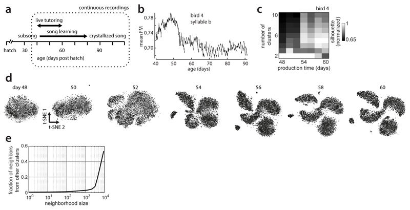
Extended Data Figure 1. Clustering of juvenile and adult zebra finch song.

(a) Vocal development in male zebra finches. Tutoring by an adult male started around day 46 (post hatch) and lasted 10-20 days.

(b) Time course of the acoustic feature frequency modulation, for syllable b in the example bird (compare Fig. 1b).

(c) Normalized mean silhouette values for 2-10 clusters for vocalizations from the 7 days in (d). High values indicate evidence for the respective cluster count. Mean normalized silhouette coefficients are based on 20 repetitions of k-means clustering of random subsets of 1000 68ms onset-aligned spectrogram segments from a single day (same as in d) projected onto the first 5 principal components.

(d) t-SNE visualizations of vocalizations produced on a given day post hatch (labels) for the example bird. A separate embedding was computed for each day and the embedding’s initial condition was based on the previous day. Note the gradual emergence of clusters, each corresponding to a distinct syllable type (e.g. syllables i, a, b, c in Fig. 2a).

(e) Average fraction of neighbors from a different cluster, as a function of neighborhood size. Analogous data to (c) and (d) but for vocalizations from day 90 (12,854 data points), when clusters are fully developed. For a wide range of neighborhood sizes, the neighbors of a data point mostly belong to the same cluster or syllable type. For a neighborhood size of 100, the average fraction of out-of-cluster neighbors from the same day is 0.0089. For an appropriately chosen neighborhood size, nearest neighbor methods thus respect clustering structure in the data by construction and sidestep having to explicitly identify clusters in the data. In most analyses, we computed nearest neighbors on data from all days, meaning that clustering structure is respected even for neighborhood sizes somewhat larger than those implied in (e).

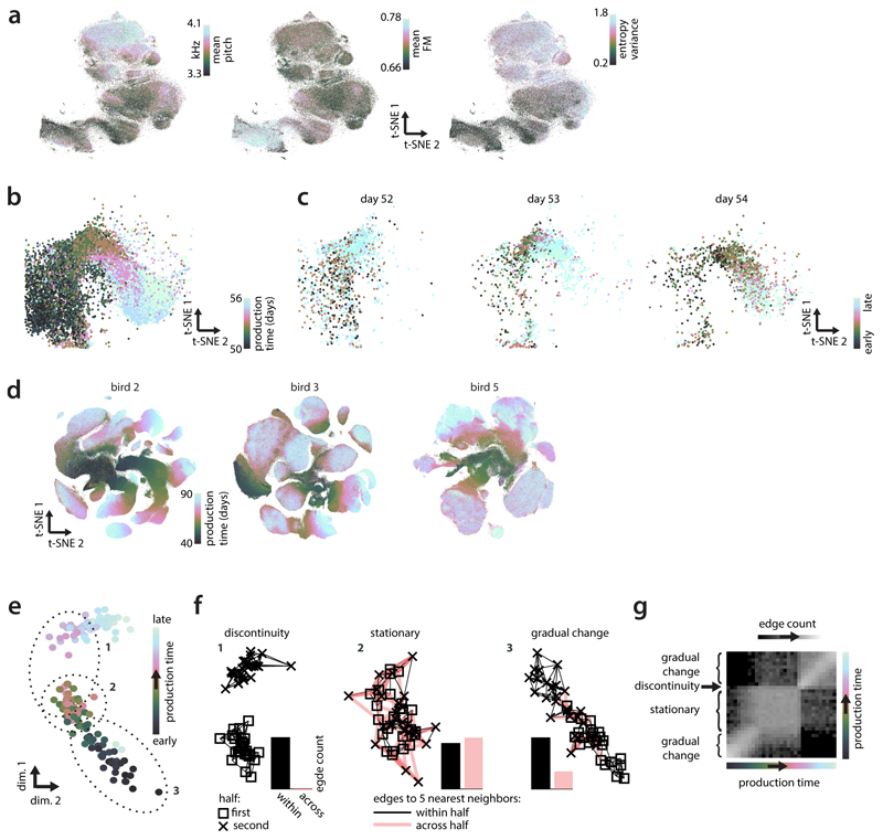
Extended Data Figure 2. Properties of large-scale embeddings.

(a) Three auditory features computed on renditions of syllable b. Same embedding as in Fig. 2a, but different coloring.

(b) Across-day change in vocalizations. Magnified cutout from Fig. 2a (bottom-left region of the dashed square). Coloring differs from Fig. 2a and only points from days 50-56 are shown.

(c) Within-day change in vocalizations. Points from (b) are shown separately for three individual days (top labels) and colored based on production time within the day (early to late; color bar). Vocalizations change within a day—early vocalizations (dark green) are more similar to vocalizations from previous days (dark green points in b); late vocalizations (light blue) are more similar to vocalization from future days (light blue in b).

(d) t-SNE visualizations for the continuous recordings of 3 birds (columns). Analogous to Fig. 2a.

(e-g) Illustration of a fictitious behavior undergoing distinct phases of abrupt change, no change, and gradual change, and the identification of these phases based on nearest neighbor graphs.

(e) A low-dimensional representation of the behavior. Each point corresponds to a behavioral rendition (e.g. a syllable rendition in the bird data) and is colored based on its production time. Similar renditions (e.g. that have similar spectrograms) appear near each other in this representation. The dotted ellipses mark three subsets of points corresponding to (1) a phase of abrupt change; (2) a phase of no change; and (3) a phase of gradual change.

(f) Nearest neighbor graphs for the three subsets of points in (e). Points are replotted from (e) with different symbols, indicating whether their production times fall within the first (squares) or second half (crosses) of the corresponding subset. Edges connect each point to its 5 nearest neighbors. Edge color marks neighboring pairs of points falling into the same (black) or different (red) halves. Relative counts of within- and across-half edges differ based on the nature of the underlying behavioral change (histograms of edge counts). If an abrupt change in behavior occurs between the first and second half, nearest neighbors of points in one half will all be points from the same half, and none from the other half (discontinuity). When behavior is stationary, the neighborhoods are maximally mixed, i.e. every point has about an equal number of neighbors from the two halves (stationary). Phases of gradual change result in intermediate levels of mixing (gradual change).

(g) Mixing-matrix for the simulated data in (e), analogous to Fig. 2e. Each location in the matrix corresponds to a pair of production times. Strong mixing (white) indicates a large number of nearest neighbor edges across the two corresponding production times (as in f, stationary) and thus similar behavior at the two times. Weak mixing (black) indicates a small number of such edges (as in f, discontinuity), and thus dissimilar behavior. Note that such statistics on the composition of local neighborhoods can be computed for any kind of behavior and are invariant with respect to transformations of the data that preserve nearest neighbors, like scaling, translation, or rotation. These properties make nearest neighbor approaches very general.

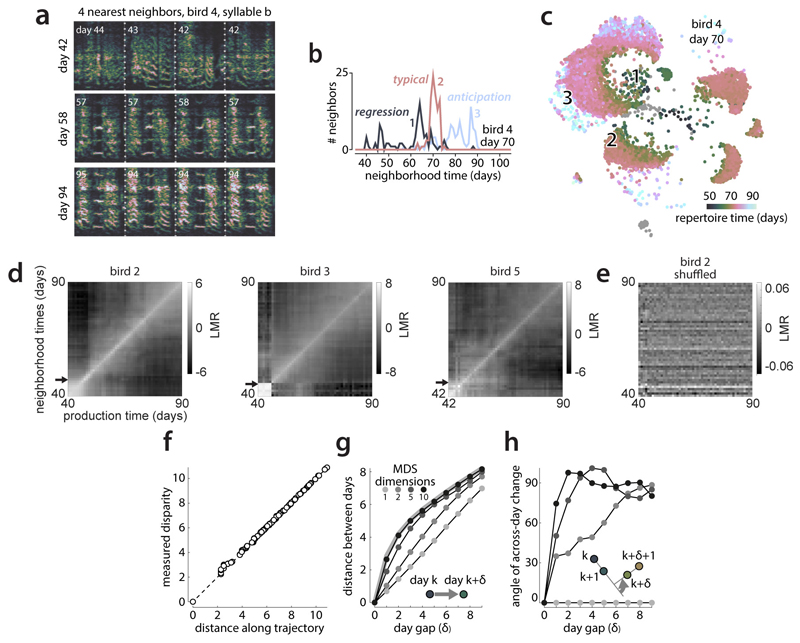
Extended Data Figure 3. Repertoire dating and the direction of slow change.

(a) The four nearest neighbors for example vocalizations (bird 4, syllable b, Fig. 1a, example syllables are marked by red lines). Production times of nearest neighbors (numbers) need not equal that of the corresponding example rendition.

(b) Neighborhood production times for three renditions from day 70 (analogous to Fig. 2a, inset). Rendition 2 is “typical” for day 70 (most neighbors lie in the same or adjacent days); renditions 1 and 3 are a “regression” and an “anticipation” (with neighbors predominantly produced in the past or future, respectively).

(c) All renditions of day 70 (subset of points from Fig. 2a). Color corresponds to repertoire time (rT, 50^th percentile in Fig. 2d). Anticipations (rT>70) and regressions (rT<70) occur at locations corresponding to vocalizations typical of later and earlier development (compare to Fig. 2a). Numbers 1-3 mark the approximate locations of the example renditions in (b).

(d) Mixing-matrices for additional birds (analogous to Fig. 2e, same birds as in Extended Data Fig. 2d). Bird 3 produced only very few vocalizations (mostly calls) before tutoring onset (black arrows). The mixing-matrices consistently show a period of gradual change starting after tutor onset and lasting several weeks. This gradual change typically slows down (resulting in larger mixing values far from the diagonal) at the end of the developmental period considered here (day 90 post hatch; later periods in Extended Data Fig. 6). Gray values correspond to the base-2 logarithm of the mixing ratio, i.e. histograms over the pooled neighborhood times (Fig. 2c) normalized by a null hypothesis obtained from a random distribution of production times (see Methods). For example, an LMR value of 5 implies that renditions from the corresponding pair of production-times are 2⁵ = 32 times more mixed at the level of local neighborhoods than expected by chance (i.e. a random distribution of production times across renditions).

(e) Like (d), bird 2, but after shuffling production times among all data points. Effects under this null hypothesis are small (the maximal observed mixing ratio is 2^0.06~1.042). Similar, small effects under the null hypothesis are obtained for the other mixing matrices discussed throughout the text.

(f-h) Properties of the behavioral trajectory inferred from the mixing-matrix in Fig. 2f.

(f) Pairwise distances between points along the inferred behavioral trajectory (x-axis) compared to the measured disparities (y-axis). Disparities are obtained by rescaling and inverting the similarities in Fig. 2f (see Methods). The points on the trajectory are inferred with 10-dimensional non-metric multidimensional scaling (MDS) on the measured disparities. Crucially, the pairwise distances between inferred points faithfully represent the corresponding, measured disparities (all points lie close to the diagonal; MDS stress = 0.0002).

(g, h) Structure of low-dimensional projections of the behavioral trajectory. We applied principle component analysis to the 10-d arrangement of points inferred with MDS and retained an increasing number of dimensions (number of dimensions indicated by gray-scale). For example, the projection onto the first two principle components is shown in Fig. 2h (MDS dimensions 2 in (g) and (h)). The first two principle components explain 75% of the variance in the full 10-d trajectory.

(g) Measured disparity (thick gray curve) and distances along the inferred trajectories (points and thin curves) as a function of the day-gap δ between points. For any choice of projection dimensionality and δ, we computed the Euclidean distances between any two points separated by δ and averaged across pairs of points. The measured disparities increase rapidly between subsequent and nearby days, but only slowly between far apart days (thick gray curve). Low dimensional projections of the trajectory (e.g. MDS dimensions 2) underestimate the initial increase in disparities.

(h) Angle between the reconstructed direction of across-day change for inferred behavioral trajectories, as a function of the day-gap between points. Same conventions and legend as in (f). For the 1-d and 2-d trajectories, the direction of across-day change varies little or not at all from day to day (see inset, arrow indicates angle of across-day change). On the other hand, the direction of across-day change along the full, 10-d behavioral trajectory is almost orthogonal for subsequent days. Both (g) and (h) imply that the full behavioral trajectory is more “rugged” than suggested by the 2d-projection in Fig. 2h. This structure is consistent with the finding that across-day change includes a large component that is orthogonal to the directions of slow change and of within-day change (Fig. 3j). Note that (a) is based on 200ms spectrogram segments whereas b-h are based on 68ms segments (like most of the analyses).

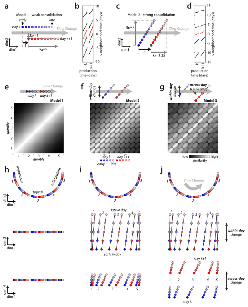
Extended Data Figure 4. Models of the alignment between components of change.

(a-d) Validation of repertoire dating. We simulated individual behavioral renditions as points in a high-dimensional space, drawn from a time-dependent probability distribution changing both within and across days (see Methods) and verified that repertoire dating can successfully recover the underlying structure of the models. The main parameters determining the relative alignment of the direction of slow change (DiSC) with the directions of within-day and across-day change are k_a, the amount of within-day change along the DiSC; g_n, the amount of within-day change orthogonal to the DiSC; and b_n, the amount of across-day change orthogonal to the DiSC. These parameters are expressed relative to the amount of across-day change along the DiSC (thick black arrow in (a) and (b)). The two models shown imply different amounts of overnight consolidation of within-day changes along the DiSC.

(a) Schematic illustration of model 1. Within-day change is aligned with the DiSC (g_n=0) and large (k_a=5). The component of across-day change orthogonal to the DiSC is as large as the component of across-day change along it. In this scenario, overnight consolidation of within-day changes along the DiSC is weak for typical renditions (20% of change is consolidated, corresponding to a consolidation index of -0.8 in Fig. 1).

(b) Repertoire dating percentiles for model 1, analogous to Fig. 3b. Dating of the typical renditions (red) closely reproduces dynamics of change along the DiSC implied by (a)—within-day change along the DiSC is large (red line extends over about 5 days) and consolidation is weak (starting point on day k+1 relative to day k moves by about 20% of overall within-day range).

(c) Schematic illustration of model 2. Within-day change has a large component orthogonal to the DiSC, whereas across-day change is aligned with the DiSC. In this scenario, overnight consolidation of within-day changes along the DiSC is strong (80% of the change is consolidated; consolidation index -0.2) for typical renditions.

(d) Repertoire dating percentiles for model 2, analogous to (b). Dating of the typical renditions (red) closely reproduces dynamics of change along the DiSC implied by (c). In (b) and (d), differences between anticipations (95^th percentile) and regressions (5^th percentile) correctly reflect the underlying model parameters (see Methods).

(e-j) Validation of stratified behavioral trajectories. We generated 3 sets of stratified behavioral trajectories that differ with respect to the alignment of within-day and across-day change with the DiSC. We built each set of trajectories by arranging 50 points (5 strata per day, 5 production-time periods per day, on 2 consecutive days; same conventions as Fig. 3f,g) within a 4-dimensional space. We then generated simulated stratified mixing matrices (e-g, replotted from Fig. 3f) by computing pairwise distances between all points, and transforming distances into similarities. We visualize the behavioral trajectories (h-j) with the same 2-d projections as in Fig. 3h-j, with the same scale along all dimensions. In all models, overnight consolidation along the DiSC is perfect for all strata.

(e) Model 1: within-day change and across-day change occur only along the DiSC. For each stratum (i.e. each of the five 10-by-10 squares along the diagonal) similarity decreases smoothly with time, reflecting the gradual progression of the trajectory along the DiSC within and across days.

(f) Model 2: within-day change has a large component that is not aligned with the DiSC.

(g) Model 3: both within-day and across-day change have large components that are not aligned with the DiSC. The misaligned component of across-day change reduces the similarity between day k and day k+1 compared to model 2, resulting in smaller values in the 5-by-5 squares comparing points from day k and day k+1.

(h) Behavioral trajectories for model 1: the 2-d projection containing the DiSC (top) explains all the variance in the trajectories.

(i) Behavioral trajectories for model 2: similar to (h), but points from different periods during the day are displaced also along an orthogonal direction of within-day change (middle).

(j) Behavioral trajectories for model 3: similar to (i), but points from adjacent days are displaced also along an orthogonal direction of across-day change (bottom). Note that the models in (e-f) are implemented differently than the models in (a-d) (see Methods).

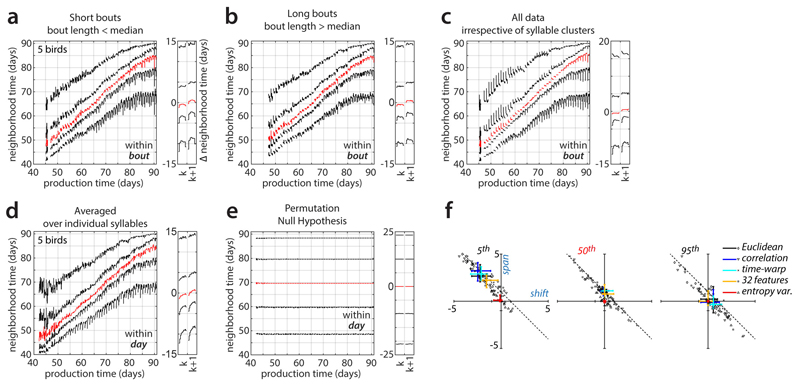
Extended Data Figure 5. Repertoire dating control analyses.

(a-c) Within-bout effects, analogous to Fig. 3c,d.

(a) Within-bout effects computed only from renditions falling into short bouts (bout length < median).

(b) Analogous to (a), but computed only from renditions falling into long bouts (bout length > median). The changes in the behavioral repertoire observed within a bout are qualitatively similar for short and long bouts (compare (a) and (b); within-bout effects are most pronounced after day 70). In particular, the song becomes more regressive shortly before the end of a bout (5^th percentile, bottom curves). This finding suggests that the analogous effect in Fig. 3c,d occurs at the end of a bout rather than at a fixed time after the beginning of a bout.

(c) Analogous to Fig. 3c,d but computed over the entire data set without prior clustering into syllables. The changes in behavioral repertoire differ in several respects from those in Fig. 3c,d, which were computed on individual syllables and then averaged across syllables (see Methods). In (c), the increase in regressions at bout end is less pronounced. Moreover, large within-bout changes occur also for anticipations early during development. Both differences may reflect changes in the relative frequency of renditions from each syllable (e.g. introductory notes) sung throughout a bout. Such changes in frequency can affect the results in (c), which were computed on the un-clustered data, but not those in (a) and (b).

(d) Within-day effects, analogous to Fig. 3a,b, but computed for individual syllables, and then averaged across syllables and animals. The changes in behavioral repertoire are qualitatively similar to those in Fig. 3a,b, which were computed un the un-clustered data. This similarity implies that the dynamics along the direction of slow change in Fig. 3 cannot be explained by changes during the day in the relative frequency of renditions from each syllable.

(e) Analogous to Fig. 3a,b but computed after shuffling production times among all data points. Within-day changes of the percentile curves are small under this null hypothesis. The maximal span of within-day fluctuations is 0.2 days, compared to 3.71 for the unshuffled data in Fig. 3b. The total repertoire spread (5^th – 95^th percentile) is around ~40 days compared to ~23 days for unshuffled data. The 50^th percentile curve is flat, implying that the shuffled data does not undergo a systematic drift over time, i.e. does not describe a direction of slow change (DiSC). The vertical separation between percentiles then reflects the range of production times in the data, not the spread along the DiSC. The time-course of the 5^th and 95^th repertoire dating percentiles should thus be interpreted as the progression of regressions and anticipations along the DiSC only over the range of repertoire times covered by typical renditions (i.e. approximately the vertical range of the 50^th repertoire dating percentile).

(f) Analogous to Fig. 3e but for different distance metrics (Euclidean; correlation; Euclidean-after-time-warping) and feature representations (32 acoustic features; 1 acoustic feature: entropy variance). See also Extended Data Fig. 9.

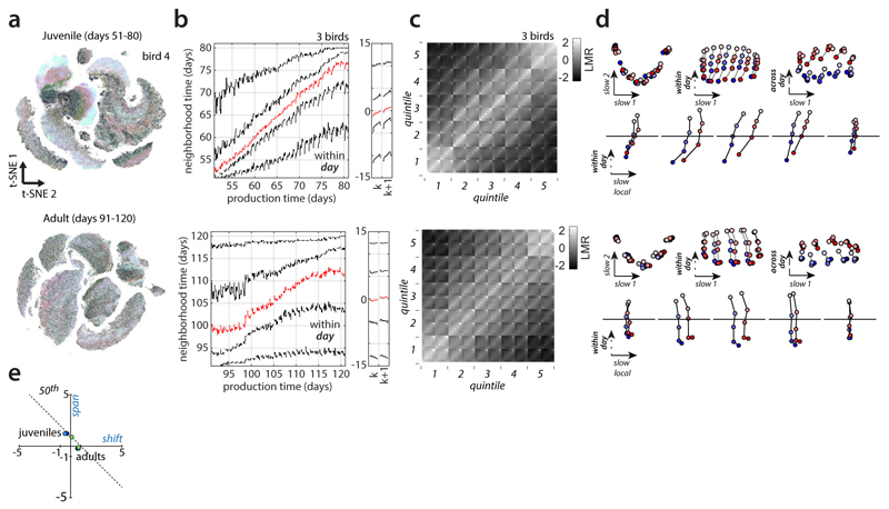
Extended Data Figure 6. Behavioral change in adult vs. juvenile birds.

(a-d) Comparison of within-day repertoire dating results during and after the end of development (average over 3 birds). Top: Juvenile birds. Bottom: Same birds but as adults.

(a) Large scale embeddings analogous to Fig. 2a.

(b) Repertoire dating percentiles, analogous to Fig. 3a,b.

(c) Stratified mixing matrix, analogous to Fig. 3g.

(d) Stratified behavioral trajectories, analogous to Fig. 3h-k.

(e) Shift and span values for the 50^th percentile, juvenile and adult birds (labels). Points indicate individual birds. Song in adult birds is not static, but the time-course of change differs from that observed in juveniles. First, change in adults is substantially smaller than in juveniles (slope of 50^th percentile in b, top vs. b, bottom). Second, the relation of fast (within-day) change and slow (across-day) change differs in juveniles vs. adults. In juveniles, vocalizations move along the DiSC (vertical axes in (b); slow local axis in (d)) within each day and the repertoire time of typical renditions increases by about 1 day from morning to evening (50^th percentile; span ≈ 1 day) and is maintained through the next morning (shift ≈ 0 days). In adults, typical renditions do not show any evidence of within-day progress along the DiSC (span≈0 days) but change overnight across days (shift > 0 days). In adults, the regressive tail of the repertoire in particular moves towards smaller values during the day (b, bottom, right; 5^th percentile), whereas in juveniles it consistently moves towards larger values (b, top). Both in juvenile and adult birds, within-day change has a strong component that is misaligned with the DiSC (within-day axis in (d)).

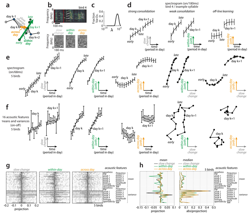
Extended Data Figure 7. Local linear analysis.

(a-e) We validated the structure of change inferred with nearest neighbor statistics (Fig. 3) with an approach based on linear regression in the high-dimensional spectrogram space (see Methods). Unlike for the case of nearestneighbor-based statics, here each rendition must first be assigned to a cluster (i.e. a syllable, compare Fig. 2a) and each cluster is analyzed separately.

(a) Illustration of the linearization scheme. First, we infer the (local) direction of slow change (DiSC) on days k and k+1 (gray arrow) as the vector of linear regression coefficients relating production day to variability of renditions from days k-1 and k+2. Second, we infer the direction of within-day change (green arrow) as the linear-regression coefficients relating the period within a day to variability of renditions from days k and k+1, orthogonalized to the DiSC. Third, we infer the direction of across-day change (orange arrow) as the linear-regression coefficients relating production day to variability of renditions from days k and k+1, orthogonalized to the DiSC and within-day change. All three sets of coefficients, and the corresponding directions in spectrogram space, typically vary across days, syllables, and birds. The progression of song along the DiSC and along the (orthogonalized) directions of within-day and across-day change are obtained by projecting renditions on day k and k+1 onto the corresponding directions.

(b) Example rendition of syllable b as in Fig. 1 (top; encapsulated by red lines) and inferred coefficients (i.e. directions in spectrogram space; bottom) for day k=57. Bright and dark shades of gray mark spectrogram bins for which power increases or decreases, respectively, over the corresponding timescales in (a).

(c) Dependency of cross-validated regression quality (fraction of variance explained) on the regularization constant for the estimation of the DiSC. One regularization constant was chosen for each syllable and direction based on maximizing the leave-one-out cross validation error on the training set.

(d) Progression of syllable b along the directions of change shown in (b), during days 57 and 58. Renditions from each day are binned into 10 consecutive periods based on production time within the day (analogous to the 10 periods in Fig. 3a,b; curves and error bars: means and 95% bootstrapped confidence intervals). For simplicity of visualization, the time elapsed (horizontal axis) during the night between days k and k+1 is not shown to scale. The position along the DiSC for the morning of day k+1 is close to that for the evening of day k, indicating overall strong consolidation (left). The position along the direction of within-day-change is reset overnight, implying that the underlying changes are not consolidated (middle). The position along the direction of across-day change jumps overnight, consistent with off-line learning (right). Notably, strong consolidation, weak consolidation, and offline learning have all been reported in the past, albeit in different behaviors and species. The panels in (d) show that these different patterns of change can occur in the very same syllable along distinct spectral features (see also Fig. 1h and Extended Data Fig. 8). By considering features with different projections onto these directions a wide range of consolidation patterns can be “uncovered” (Fig. 1h).

(e) Same as (d) but averaged across all 4-day windows during days 60-69 and over all syllables and birds (same 5 birds as in Figs. 2, 3). The resulting averages include contributions from the entire behavioral repertoire, including regressions, typical renditions, and anticipations. The two right-most panels show concurrent progression along the DiSC and the direction of within-day or across-day change, combining data from the first and second, or first and third panels in (e). These representations are analogous, and in qualitative agreement, with the behavioral trajectories in Fig. 3h-k (typical).

(f) Analogous to (e) but computed on vocalizations represented by 32 acoustic features instead of spectrograms. Directions as in (e) can be retrieved, but progression along the DiSC appears noisier, suggesting that the 32 acoustic features do not fully capture in particular the slow spectral changes occurring over development (see also Extended Data Fig. 9).

(g,h) Contribution of individual acoustic features to the directions of slow, within-day, and across-day change. As in (f), the directions are computed in the space of 32 acoustic features.

(g) Distribution of coefficients in the retrieved orthonormalized directions. Thick and thin black bars: mean and 95% confidence intervals; crosses: outliers; thin vertical lines: median.

(h) Mean (solid lines) and median (dotted lines) of the signed (left) or unsigned (right) distributions in (g). Most coefficients are small and variable, indicating that the alignment between any of the 32 acoustic features and the inferred directions of change is weak and highly variable over time, syllables, and birds.

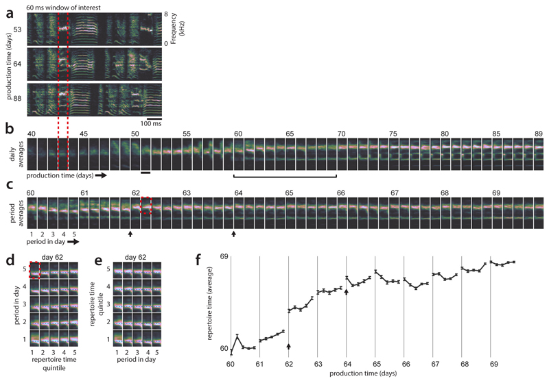
Extended Data Figure 8. Behavioral variability and stratification in an example syllable.

(a) Songs of an example bird for 3 days during development. Only spectrogram segments belonging to a particular syllable and location in the motif (68ms window of interest; red dotted lines) are analyzed in the following panels.

(b) Developmental changes over the course of weeks. Renditions are binned by production day, and averaged. The most apparent changes occurring during learning are an increase in pitch and the later, successive appearance of additional spectral lines at low frequencies.

(c) Within-day and across-day changes for days 60-69. Renditions are binned into 5 production-time periods spanning a day and averaged within bins. On many days, the changes within a day do not appear to recapitulate the changes occurring across days (e.g. days 60 and 65; within-day progression does not smoothly transition between the vocalizations on preceding and subsequent days, see b). The averages also reveal occasional overnight “jumps” in the properties of the vocalizations (e.g. black arrows).

(d) Comparison of within-day change and change on longer times-scales. Renditions within each period and day were split into strata according to their repertoire times (e.g. quintiles in Fig. 2d) resulting in 25 averages, one for each combination of stratum and period within the day. Only the upper part of the spectrogram is shown (red rectangle in c). The progression along strata (x-axis) emphasizes the large extent of motor variability along the DiSC existing within a single day (day 62).

(e) Same averages as in (d), but with x and y axes swapped. In particular for regressive renditions (quintile 1), change within day 62 (x-axis) does not recapitulate developmental changes occurring over months (x-axis in D).

(f) Repertoire dating based on repertoire time (as in Extended Data Fig. 3c). Each point corresponds to a production-time period and the average of all repertoire times of renditions in that period. Error-bars show bootstrapped 95% confidence intervals. The change in repertoire time, which is computed without using a low dimensional parametrization of vocalizations through explicit acoustic features, captures the movement along the DiSC.

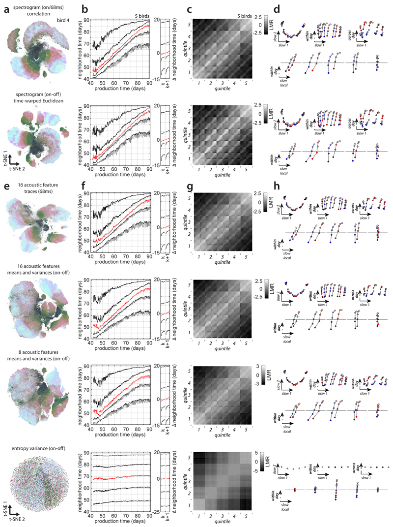
Extended Data Figure 9. Behavioral change based on alternative distance metrics and features.

To demonstrate the robustness of the proposed nearest neighbor statistics, we verified that the inferred time-course of behavioral change is reproduceable using a number of different distance metrics (used to define nearest neighbors) and parameterizations of vocalizations.

(a-d) We recomputed the main analyses using a Pearson’s correlation metric on 68ms onset-aligned spectrogram segments (first row); and the Euclidean distance on onset-to-offset spectrogram segments that were linearly time-warped to a duration of 100ms (second row). In comparison, the main analyses in the manuscript were based on Euclidean distance on 68ms onset-aligned spectrogram segments (e.g. Fig2c-f, Fig. 3).

(a) t-SNE visualization based on the corresponding distance metrics and sound representation for the example bird, analogous to Fig. 2a.

(b) Repertoire dating averaged over birds, analogous to Fig. 3a,b.

(c) Stratified mixing matrices averaged over birds, analogous to Fig. 3g. The mixing values are highly correlated across distance metrics: Euclidean (main analyses) vs. correlation: variance explained = 92%; Euclidean (main analyses) vs. time-warped-Euclidean: 93%.

(d) Stratified behavioral trajectories based on (c), analogous to Fig. 3h-k. The results in (a-d) are consistent with those in Fig. 3, showing that our findings are robust with respect to the exact definition of nearest neighbors. Moreover, the overall structure of the behavioral trajectory appears to depend only minimally on changes of tempo and spectrogram magnitude (first row: Pearson’s correlation is invariant to changes in overall magnitude of vocalizations; second row: time-warped-Euclidean distance is invariant to changes in tempo).

(e-h) We recomputed all main analyses with four additional parameterizations of vocalizations: time dependent normalized acoustic feature traces for 16 acoustic features within 68ms windows after syllable onset (1^st row); means and variances of the same 16 acoustic features over entire syllables (2^nd row); means and variances of 8 of the 16 acoustic features (3^rd row); and a one-dimensional parametrization consisting solely of entropy variance computed over entire syllables (4^th row). Feature means and variances were z-scored across all syllables. For all these parameterizations we defined nearest neighbors with the Euclidean distance.

(e) Embedding using t-SNE based on the corresponding parameterization and metric. For entropy variance alone, the embedding is locally 1 dimensional without exception (data points are larger than for the other parameterizations for better visibility). Entropy variance maps mostly smoothly onto this one-dimensional manifold (not shown).

(f) Repertoire dating averaged over birds, analogous to Fig. 3a,b. Repertoire dating based on entropy variance alone fails to reproduce most of the results in Fig. 3 obtained with spectrograms segments. The percentile curves are almost flat, indicating that renditions cannot be reliably assigned to their production times based on entropy variance alone. In this case, vertical separation between percentiles cannot be interpreted as spread along the DiSC (see Extended Data Fig. 5e). For entropy variance alone, span > 0 across all percentiles, but consolidation is consistently close to zero.

(g) Stratified mixing matrix averaged over birds, analogous to Fig. 3g. The match with the mixing matrix in Fig. 3g decreases as the dimensionality of the parameterization is reduced (spectrogram vs. time-dependent feature traces: variance explained = 93%; spectrogram vs. 16 acoustic feature means and variances: 91%; spectrogram vs. 8 acoustic feature means and variances: 84%; spectrogram vs. entropy variance: 54%).

(h) Stratified behavioral trajectories based on (g), as in Fig. 3h-k. The inferred behavioral trajectories are similar across the first three song parameterizations. However, these alternative parameterizations result in more vertical separation between percentiles in (f), suggesting that they capture the direction of slow change less well (compare to Fig. 3a and Extended Data Fig. 5e). Parameterizations of reduced dimensionality also result in progressively less defined syllable clusters in the embeddings (e, top to bottom). These observations suggest that a parameterization based on the full spectrogram is better suited to capture the different directions of change explored during development (see also Extended Data Fig. 7). Note that for entropy variance (bottom row), the projections onto the local direction of slow change (bottom panels) are highly magnified compared to the projections in the top panels.

Extended Data Figure 10. Behavioral change based on random spectrogram segments.

We recomputed all main analyses with a random segmentation of behavior that does require alignment to syllable onsets. This segmentation scheme can be applied to behavior that does not fall into temporally discrete syllables. Here each data point corresponds to a randomly chosen 68ms spectrogram snippet drawn from a period of singing. Not all song was sampled, as we used 1,000,000 non-overlapping segments for each bird (see Methods).

(a) Vocalizations of the example bird (e.g. Fig. 1a) from day 76 and example segments used for the analysis.

(b) t-SNE visualization for random segments from the example bird, based on nearest neighbors defined with respect to the Euclidean distance (left panel) and average spectrograms for different locations in the (t-SNE) embedding (right panel; analogous to Fig. 2b). Clusters corresponding to individual syllables are elongated compared to Fig. 2a. Variation along one direction within the cluster tends to account for production time (color), while variation along another direction tends to reflect the timing of segments relative to syllable onsets.

(c) Embedding from Fig. 2a (bottom) and embedding of random 68ms segments (top). Points in both embeddings are colored by cluster identity defined on onset-aligned spectrogram segments covering entire syllables (bottom). The color of each point corresponding to a random snippet (top) corresponds to the cluster identity of the surrounding syllable. Some clusters in the embedding based on random segments contain points assigned to two different syllables (e.g. black and green colors);

(d) Repertoire dating averaged over birds, analogous to Fig. 3a,b.

(e) Stratified mixing matrix averaged over birds, analogous to Fig. 3g. The mixing values are highly correlated with those in Fig. 3g (variance explained = 89%)

(f) Stratified behavioral trajectories based on (e), as in Fig. 3h-k. The results in (d-f) largely reproduce the corresponding findings obtained with onset-aligned 68ms spectrogram segments (Fig. 3) as well as with other song parameterizations (Extended Data Fig. 9). Nonetheless, the overall effect sizes are reduced, likely due to the additional variability introduced by the random position of segments relative to syllable onsets. In (d), vertical separation between 5^th and 95^th percentiles is increased and slope of 50^th percentile is reduced, suggesting a noisier representation of the direction of slow change (see Extended Data Fig. 5e) compared to onset-aligned 68ms segments (Fig. 3).

Code Availability

We provide source code for our nearest neighbor based analyses (https://github.com/skollmor/repertoireDating) and for a data-browser/data analysis GUI that we used to perform some analyses and to explore and visualize data (https://github.com/skollmor/dspace).

Data Availability

The data that support the findings of this study are available from the corresponding author upon reasonable request.

References

- 1.Brashers-Krug T, Shadmehr R, Bizzi E. Consolidation in human motor memory. Nature. 1996;382:252–255. doi: 10.1038/382252a0. [DOI] [PubMed] [Google Scholar]
- 2.Derégnaucourt S, Mitra PP, Fehér O, Pytte C, Tchernichovski O. How sleep affects the developmental learning of bird song. Nature. 2005;433:710–6. doi: 10.1038/nature03275. [DOI] [PubMed] [Google Scholar]
- 3.Tchernichovski O, Mitra PP, Lints T, Nottebohm F. Dynamics of the vocal imitation process: how a zebra finch learns its song. Science. 2001;291:2564–9. doi: 10.1126/science.1058522. [DOI] [PubMed] [Google Scholar]
- 4.Andalman AS, Fee MS. A basal ganglia-forebrain circuit in the songbird biases motor output to avoid vocal errors. Proc Natl Acad Sci U S A. 2009;106:12518–23. doi: 10.1073/pnas.0903214106. [DOI] [PMC free article] [PubMed] [Google Scholar]
- 5.Arulkumaran K, Deisenroth MP, Brundage M, Bharath AA. Deep reinforcement learning: A brief survey. IEEE Signal Processing Magazine. 2017 doi: 10.1109/MSP.2017.2743240. [DOI] [Google Scholar]
- 6.Ingram JN, Flanagan JR, Wolpert DM. Context-Dependent Decay of Motor Memories during Skill Acquisition. Curr Biol. 2013;23:1107–1112. doi: 10.1016/j.cub.2013.04.079. [DOI] [PMC free article] [PubMed] [Google Scholar]
- 7.Klaus A, et al. The Spatiotemporal Organization of the Striatum Encodes Action Space. Neuron. 2017;95:1171–1180.:e7. doi: 10.1016/j.neuron.2017.08.015. [DOI] [PMC free article] [PubMed] [Google Scholar]
- 8.Han S, Taralova E, Dupre C, Yuste R. Comprehensive machine learning analysis of Hydra behavior reveals a stable basal behavioral repertoire. Elife. 2018;7 doi: 10.7554/eLife.32605. [DOI] [PMC free article] [PubMed] [Google Scholar]
- 9.Egnor SER, Branson K. Computational Analysis of Behavior. Annu Rev Neurosci. 2016;39:217–236. doi: 10.1146/annurev-neuro-070815-013845. [DOI] [PubMed] [Google Scholar]
- 10.Wiltschko AB, et al. Mapping Sub-Second Structure in Mouse Behavior. Neuron. 2015;88:1121–1135. doi: 10.1016/j.neuron.2015.11.031. [DOI] [PMC free article] [PubMed] [Google Scholar]
- 11.van der Maaten L. Accelerating t-SNE using Tree-Based Algorithms. J Mach Learn Res. 2014;15:3221–3245. [Google Scholar]
- 12.Chen H, Friedman JJH. A new graph-based two-sample test for multivariate and object data. J Am Stat Assoc. 2016;1459:1–41. [Google Scholar]
- 13.Hawks M. Graph-theoretic statistical methods for detecting and localizing distributional change in multivariate data. 2015 [Google Scholar]
- 14.Kruskal JB. Multidimensional scaling by optimizing goodness of fit to a nonmetric hypothesis. Psychometrika. 1964;29:1–27. [Google Scholar]
- 15.Shank SS, Margoliash D. Sleep and sensorimotor integration during early vocal learning in a songbird. Nature. 2009;458:73–7. doi: 10.1038/nature07615. [DOI] [PMC free article] [PubMed] [Google Scholar]
- 16.Fenn KM, Nusbaum HC, Margoliash D. Consolidation during sleep of perceptual learning of spoken language. Nature. 2003;425:614–616. doi: 10.1038/nature01951. [DOI] [PubMed] [Google Scholar]
- 17.Tchernichovski O, Nottebohm F, Ho C, Pesaran B, Mitra P. A procedure for an automated measurement of song similarity. Anim Behav. 2000;59:1167–1176. doi: 10.1006/anbe.1999.1416. [DOI] [PubMed] [Google Scholar]
- 18.Anderson DJJ, Perona P. Neuron. Vol. 84. Cell Press; 2014. Toward a science of computational ethology; pp. 18–31. [DOI] [PubMed] [Google Scholar]
- 19.Krakauer JW, Shadmehr R. Consolidation of motor memory. Trends Neurosci. 2006;29:58–64. doi: 10.1016/j.tins.2005.10.003. [DOI] [PMC free article] [PubMed] [Google Scholar]
- 20.Brainard MS, Doupe AJ. What songbirds teach us about learning. Nature. 2002;417:351–8. doi: 10.1038/417351a. [DOI] [PubMed] [Google Scholar]
- 21.Catchpole CK, Slater PJB. Bird Song: Biological Themes and Variations. 2003 [Google Scholar]
- 22.Dhawale AK, Smith MA, Ölveczky BP. The Role of Variability in Motor Learning. Annu Rev Neurosci. 2017;40:479–498. doi: 10.1146/annurev-neuro-072116-031548. [DOI] [PMC free article] [PubMed] [Google Scholar]
- 23.Lipkind D, et al. Songbirds work around computational complexity by learning song vocabulary independently of sequence. Nat Commun. 2017;8:1247. doi: 10.1038/s41467-017-01436-0. [DOI] [PMC free article] [PubMed] [Google Scholar]
- 24.Korman M, et al. Daytime sleep condenses the time course of motor memory consolidation. Nat Neurosci. 2007;10:1206–1213. doi: 10.1038/nn1959. [DOI] [PubMed] [Google Scholar]
- 25.Fischer S, Hallschmid M, Elsner AL, Born J. Sleep forms memory for finger skills. Proc Natl Acad Sci U S A. 2002;99:11987–91. doi: 10.1073/pnas.182178199. [DOI] [PMC free article] [PubMed] [Google Scholar]
- 26.Fehér O, Wang H, Saar S, Mitra PP, Tchernichovski O. De novo establishment of wild-type song culture in the zebra finch. Nature. 2009;459:564–568. doi: 10.1038/nature07994. [DOI] [PMC free article] [PubMed] [Google Scholar]
- 27.Adam I, Elemans CPH. Vocal Motor Performance in Birdsong Requires Brain-Body Interaction. eNeuro. 2019;6 doi: 10.1523/ENEURO.0053-19.2019. [DOI] [PMC free article] [PubMed] [Google Scholar]
- 28.Walker MP, Brakefield T, Allan Hobson J, Stickgold R. Dissociable stages of human memory consolidation and reconsolidation. Nature. 2003;425:616–620. doi: 10.1038/nature01930. [DOI] [PubMed] [Google Scholar]
- 29.Vogelstein JT, et al. Discovery of brainwide neural-behavioral maps via multiscale unsupervised structure learning. Science. 2014;344:386–92. doi: 10.1126/science.1250298. [DOI] [PubMed] [Google Scholar]
- 30.Fahad A, et al. A survey of clustering algorithms for big data: Taxonomy and empirical analysis. IEEE Trans Emerg Top Comput. 2014;2:267–279. [Google Scholar]
Associated Data
This section collects any data citations, data availability statements, or supplementary materials included in this article.
Supplementary Materials
Data Availability Statement