Abstract
We propose a forward-backward splitting algorithm to integrate deep learning into maximum-a-posteriori (MAP) positron emission tomography (PET) image reconstruction. The MAP reconstruction is split into regularization, expectation-maximization (EM), and a weighted fusion. For regularization, the use of either a Bowsher prior (using Markov-random fields) or a residual learning unit (using convolutional-neural networks) were considered. For the latter, our proposed forward-backward splitting EM (FBSEM), accelerated with ordered subsets (OS), was unrolled into a recurrent-neural network in which network parameters (including regularization strength) are shared across all states and learned during PET reconstruction. Our network was trained and evaluated using PET-only (FBSEM-p) and PET-MR (FBSEM-pm) datasets for low-dose simulations and short-duration in-vivo brain imaging. It was compared to OSEM, Bowsher MAPEM, and a post-reconstruction U-Net denoising trained on the same PET-only (Unet-p) or PET-MR (Unet-pm) datasets. For simulations, FBSEM-p(m) and Unet-p(m) nets achieved a comparable performance, on average, 14.4% and 13.4% normalized root-mean square error (NRMSE), respectively; and both outperformed OSEM and MAPEM methods (with 20.7% and 17.7% NRMSE, respectively). For in-vivo datasets, FBSEM-p(m), Unet-p(m), MAPEM, and OSEM methods achieved average root-sum-of-squared errors of 3.9%, 5.7%, 5.9%, and 7.8% in different brain regions, respectively. In conclusion, the studied U-Net denoising method achieved a comparable performance to a representative implementation of the FBSEM net.
Index Terms: Deep learning (DL), image reconstruction, MRI, positron emission tomography (PET)
I. Introduction
MODEL-BASED image reconstruction of positron emission tomography (PET) has now almost superseded conventional reconstruction methods by accounting for all statistical and physical processes of data acquisition in the image reconstruction. Founded on a Bayesian framework, these techniques can even model the prior probability distribution of the unknown activity distribution. Different image priors have been proposed in the literature, particularly to suppress noise in the reconstructed images without compromising image quality [1]. Based on Markov random fields, the majority of these priors aim to assign a low probability to images that have large local intensity differences between their voxels based on the hypothesis that those differences are due to noise. The major limitation of these hypothesis-driven priors is that they might not only suppress noise but also legitimate image details and boundaries, depending on the strength of hyperparameters chosen before reconstruction. Thus, edgepreserving and anatomically informed priors have been used to reduce noise while preserving PET details [2]–[5]. However, their performance highly depends on their functional form and hyperparameters, which are often hand-engineered and selected before reconstruction.
Machine learning and deep learning (DL) and techniques have recently shown promise in many aspects of PET imaging from photon detection to image reconstruction and quantification [6], [7]. In particular, deep convolutional-neural networks (CNNs) have an immense potential to learn most representative image features from a multimodal training space and hence give rise to data-driven priors which can surpass hypothesis-driven ones.
Recent developments for leveraging supervised DL techniques in PET image reconstruction can be categorized into three groups: 1) direct mapping of PET sinograms to PET images using end-to-end neural networks [8], [9]; 2) image enhancement of PET images in terms of noise [10], [11] or convergence [11], [12]; and 3) model-based DL reconstruction, which combines DL with conventional model-based reconstruction methods [13]. Direct techniques aim to learn the whole process of image reconstruction including the PET system matrix, using fully connected as well as convolutional layers, resulting in a complex learning task for which a large and diverse training corpus is presumably required. Image enhancement techniques aim to map low-dose (LD) or low-resolution or underconverged images to their target full-dose, high-resolution, and fully converged images using CNNs. On the other hand, DL reconstruction networks aim to merge the power of model-based Bayesian algorithms with neural networks through unrolling an iterative optimization algorithm, which provides an elegant theoretical foundation for designing robust data correction and image prior models.
Gong et al. [13] proposed an unrolled network, based on the alternating direction method of multipliers (ADMM) algorithm, which alternates between PET maximum-likelihood expectation-maximization (MLEM) reconstruction and supervised learning of a deep image prior using a U-Net model [14]. Gong et al. [15] further explored unsupervised learning of this network using MR images and noisy PET images as inputs and targets, respectively. To ensure the convergence of the network, the ADMM’s penalty parameter was experimentally chosen and U-Net’s parameters were initialized using separately reconstructed PET images. Cui et al. [16] used a similar deep image prior for unsupervised denoising of PET images. For an optimally chosen number of training iterations (epochs), it was shown this method outperformed a number of known denoising methods.
Lim et al. [17] proposed a DL reconstruction network by unrolling a block coordinate descent (BCD) algorithm, which alternates between MLEM PET reconstruction and iterationdependent denoising modules that are composed of convolution, soft thresholding (as an activation function), and deconvolution layers. The network’s regularization hyperparameter was finely tuned to achieve the highest contrast-to-noise ratio (CNR).
In this work, we 1) propose an optimization algorithm for Bayesian maximum-a-posteriori (MAP) PET image reconstruction, which generalizes De Pierro’s MAPEM algorithm [18] for any differentiable convex prior; 2) unroll the resulting algorithm into a model-based deep reconstruction network in which CNNs are used to learn image features while activity images are reconstructed from emission data; 3) learn any hyperparameter from data; 4) optionally incorporate anatomical side information into PET reconstruction without substantial suppression of PET unique features as seen with conventional MR-guided reconstruction algorithms; and importantly 5) investigate whether deep reconstruction methods can outperform DL-based denoising methods and whether the redesign of the current reconstruction workflow for PET scanners is justified, which would be required for clinical deployment. In this article, the proposed deep reconstruction network was evaluated using realistic 3-D brain simulations and in-vivo PET-MR scans and was compared with conventional ordered subsets expectation-maximization (OSEM), MR-guided MAPEM, and DL-based denoising using PET only and PET-MR input channels.
II. Material and Methods
A. Forward-Backward Splitting Expectation-Maximization
The Bayesian MAP reconstruction of PET emission data is obtained by the following maximization:
| (1) |
where L is the Poisson log likelihood of measured data, y, given an activity distribution, x. H is PET system matrix and is the expected accidental coincidences. R is a penalty function that imposes prior information about x, controlled by the regularization parameter β. Equation (1) can be solved using optimization transfer techniques as long as a separable, differentiable, and convex surrogate can be defined for R. Consequently, a monotonically convergent MAP expectation-maximization (EM) algorithm is obtained [18]. In this work, we use a forward-backward splitting (FBS) algorithm [19] for solving (1) for any differentiable convex prior. The FBS algorithm in fact generalizes the projected gradient descent (also known as Landweber algorithm) by substituting its projection operator with a proximal mapping operator. As a result, the optimization is performed in the following steps:
| (2) |
| (3) |
Equation (2) is the gradient descent minimization of R with the step size of γ, whereas (3) is a proximal mapping [19] associated with the log likelihood L with 1/γ as a regularization hyperparameter that controls the data fidelity of x to y and its proximity to The quadratic prior in (3) is separable. Following [20], a separable surrogate is then defined for the function L, whereby (3) can be rewritten as:
| (4) |
where is given by the following MLEM update:
| (5) |
By setting the derivative of the objective function of (4) to zero, a closed-form solution is obtained as follows [21]:
| (6) |
Algorithm 1 summarizes the resulting forward-backward splitting EM (FBSEM) algorithm, which is accelerated by the ordered subsets (OS) method. As a result, the optimization of (1) is split into three steps: 1) the regularization of the previous image estimate (7); 2) the EM update of the previous image estimate (8); and 3) the fusion of the resulting two images (9), weighted by γ and the subset-dependent sensitivity image s (m).
Algorithm 1 can be used for the following commonly used quadratic prior, weighted by MR information (wjb):
Algorithm 1. FBSEM for MAP PET Image Reconstruction.
Initialize: x (0,1) = 1, number of iterations (Nit) and subsets (Nsub)
For n = 1,…, Nit
For m = 1,…,Nsub
| (7) |
| (8) |
| (9) |
End
End
| (10) |
where 𝒩j is a neighborhood of voxels around the jth voxels. For this prior, by setting β = (1/2) and γ = [1/(Σb wjb)] in (7),we obtain
| (11) |
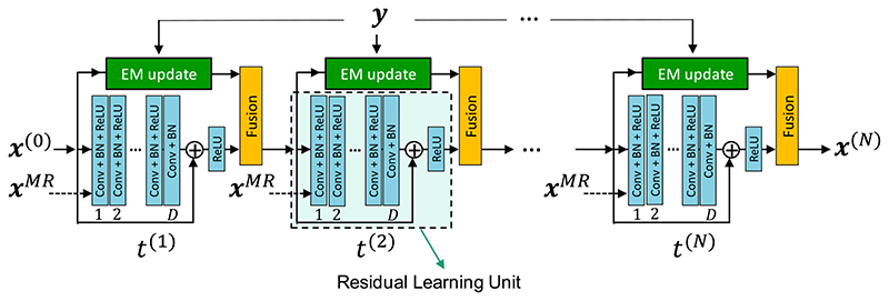
where by Algorithm 1 is reduced to De Pierro’s MAPEM algorithm [18]. As γ→∞, this algorithm reduces to the OSEM algorithm. In this article, we used a CNN-based model for R and unrolled the FBSEM algorithm into an recurrent-neural network (RNN) with N = Nit x N sub reconstruction states, in which model parameters are shared across all states, hence the number of trainable parameters became independent of the number of reconstruction updates [22]. As shown in Fig. 1, a D-layer learning unit with a non-negativity constraint [imposed by a final rectified linear unit (ReLU) layer] was used, whereby (7) was converted to a residual learning unit [23]. Of course, alternative CNN models such as convolutional encoder-decoders (e.g., U-Net [14]) could also be used.
Fig. 1.
Architecture of the proposed network using an RLU with D layers of convolution (Conv) filters, BN, and ReLU. All trainable parameters, including the regularization parameter, which is the only trainable parameter in the fusion block, are shared across all reconstruction states (t). In this network, a co-registered MR image can be optionally used as a second input channel to each state.
The proposed network was trained in a supervised manner using a training dataset composed of Ns reference highdefinition high-dose (HD) PET images , low-definition LD PET sinograms and optionally co-registered MR images The training was formulated as the minimization of the mean-squared-error loss function between the network’s output and the reference image :
| (12) |
where model parameters, θ ∈ ℝd, include convolution kernels, biases, batch normalization (BN) parameters, and γ. x (0) is an initial image estimate. Equation (12) was optimized using the Adam optimizer.
B. Simulation and In-Vivo Datasets
T1-weighted MPRAGE MR images of 70 epilepsy and dementia patients, referred for PET-MR brain imaging at PET Centre St. Thomas’s Hospital in London, were used for generating realistic brain PET-MR phantoms. The MR image matrix and voxel sizes were 230 × 230 × 254 and 1.04 × 1.04 × 1.01 mm3, respectively. The images were segmented into gray matter (GM), white matter (WM), cerebrospinal fluid (CSF), skull, and skin using the SPM12 software.1 For each dataset, an FDG PET phantom was generated as follows. Random uptake values of 96.0 ± 5.0 and 32.0 ± 5.0 (arbitrary units) were, respectively, assigned to GM and WM regions, leading to uptake ratio of 3:1 between GM and WM. Low values (>16) were assigned to the remaining regions. Four circular lesions with random radii in 2-8 mm (uniformly distributed) and random locations were generated with the hot-to-cold ratio of 50%. The uptake value of 144.0 (1.5× of GM) was assigned to hot lesions and 48.0 (0.5× of WM) was assigned to cold ones. An attenuation map was also generated by assigning attenuation values of 0.13, 0.0975, and 0 cm-1 to skull, tissues, and air, respectively. The PET, attenuation map, and T1-MR images were resampled into the voxel sizes and field of view of the standard PET images from the Siemens mMR scanner, with matrix and voxel sizes of 344 × 344 × 128 and 2.08 × 2.08 × 2.03 mm3, respectively.
For data augmentation, the resulting images were rotated in the axial direction with three random angles within [0, 15] degrees, resulting in 210 datasets. Noisy sinograms were then generated, using image-space point-spread-function (PSF) modeling in the forward model, attenuation, normalization, and Poisson noise. Random and scatter coincidences were not modeled. Each sinogram had a matrix size of 344 (radial bins) × 252 (azimuthal angles) × 837 (sinogram plans), as per the standard sinogram format for the mMR scanner.
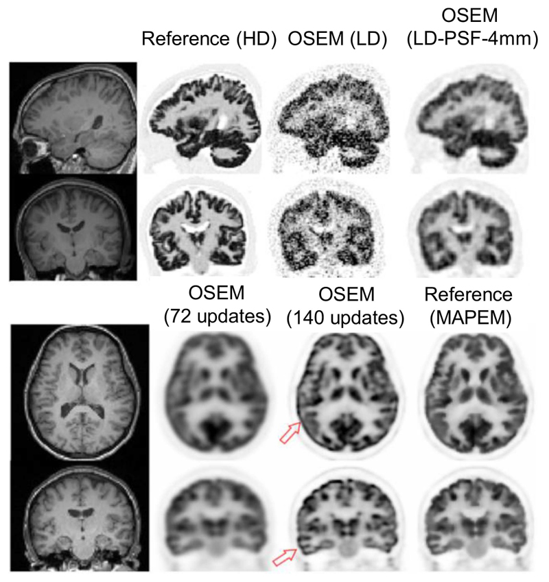
For each dataset, a high-definition HD sinogram and a low-definition LD sinogram were generated. For HD sinograms, 1 billion counts and a PSF with 2.5-mm full-width-at-half-maximum (FWHM) Gaussian kernels were considered, while for LD ones randomly chosen count levels in [90-120] million with PSF of 4.5-mm FWHM were considered. The HD data were reconstructed using the OSEM algorithm with Nit = 10, N sub = 14, and PSF = 2.5 mm to generate a reference image. The LD data were reconstructed using the same number of updates with and without PSF modeling (PSF = 4 mm) and with post-reconstruction Gaussian filtering (4-mm FWHM). Fig. 2, top, shows one simulated example dataset. For in-vivo datasets, 45 PET-MR brain datasets of patients suspected of epilepsy and dementia were retrospectively collected from our PET centre in St. Thomas’s Hospital. Following the injection of ~220 MBq [18F]FDG and uptake time of 60 min, patients underwent a simultaneous T1-MPRAGE MR scan and a 30-min PET scan on a Siemens mMR scanner. MR acquisition and parameters were as follows: repetition time: 1700 ms, echo time: 2.63 ms, inversion time: 900 ms, number of averages: 1, flip angle: 9°, and acquisition time of 382 s. For PET attenuation correction, a standard Dixon sequence and a UTE sequence was performed. The MR images were rigidly registered to PET images using SPM12 with default co-registration parameters and normalized mutual-information cost function.
Fig. 2.
Top: Reference high-definition HD images and reconstructed low-definition LD images of a sample simulation dataset. Bottom: Full-dose (30-min) images of an in-vivo dataset reconstructed using 72 EM updates (vendor’s default) and 140 updates. Increasing the number of updates improved the convergence but led to PSF Gibbs artifacts (see arrows). Thus, MR-guided MAPEM (210 updates) was used as a reference.
The datasets were split into 35 training and ten test ones. PET list-mode data were histogrammed into full-dose 30-min sinograms and LD 2-min sinograms. For one test dataset, the list-mode data were further histogrammed into 1-min and 30-s sinograms. To obtain an HD reference image, the full-dose sinograms were reconstructed with PSF modeling (using image-space 4-mm FWHM Gaussian kernels) and an MR-guided MAPEM algorithm with a quadratic prior (10), weighted using the Bowsher method [24] with 𝒩 of 3 × 3 × 3. The FBSEM algorithm was used for optimization. The regularization parameter β was chosen to be as small as possible while still mitigating PSF Gibbs-like artifacts.
Fig. 2, bottom, shows a full-dose (30-min) brain scan of a subject reconstructed by 1) OSEM using 72 updates followed by 5-mm Gaussian smoothing (Siemens e7 tools’ default); 2) OSEM with 140 updates; and 3) MR-guided MAPEM with 210 updates. As shown the default reconstruction suffers from oversmoothing and lack of convergence, while increasing the number of updates improved the convergence at the cost of PSF overshoot artifacts (see arrows). The MAPEM image shows less artifacts.
C. Network Training
In this study, the proposed FBSEM was trained and evaluated in two modes: one with PET-only inputs (FBSEM-p) and one with both PET and MR inputs (FBSEM-pm). For comparison purposes, we also included a post-reconstruction U-Net denoising model trained on the same datasets with two modes: using PET only (Unet-p) and then using both PET and MR (Unet-pm) input images. For this purpose, the original U-Net proposed in [14] was extended to 3-D with two modifications: inclusion of BN before ReLU activation and using trilinear upsampling in the decoder part of the network. The FBSEM and U-Net networks were trained in supervised learning sessions using both simulation and in-vivo training datasets. Each training dataset consists of an LD sinogram, attenuation and normalization correction factors, scatter and random sinograms, reference (HD/full-dose) PET images, LD PET images, and co-registered MR images. All sinograms were generated using Siemens e7 tools. All reference and LD sinograms were corrected for frame length and radionuclide decay before reconstruction, hence the resulting PET images were in counts-per-second units and had a similar dynamic range, which helped accelerate the training of the networks.
Table I summarizes the number of training and test datasets used for the training of the networks together with other parameters that were experimentally chosen. In this table, depth refers to the number of layers in the FBSEM net (see Fig. 1) and the number of resolution levels (or scales) in U-Net. Both networks were implemented in PyTorch and trained on a workstation equipped with a Nvidia Quadro k6000 12-GB graphic card. Thanks to the parallelism of the FBSEM net, the EM-update module was implemented in Python using a GPU-enabled PET projector, while regularization and fusion modules (with trainable parameters) were implemented in PyTorch with GPU acceleration.
Table I. Training/Test Datasets, Model Architectures, and Training Parameters Used in This Study.
| EXPERIMENT | MODEL | NO. TRAINING DATASETS | NO. TEST DATASETS | No. KERNELS IN 1st LAYER | KERNEL SIZE | DEPTH* | NO. TRAINABLE PARAMETERS | NO. BATCHES | LEARNING RATE | NO. EPOCHS | OPTIMISER | LOSS FUNCTION |
|---|---|---|---|---|---|---|---|---|---|---|---|---|
| UNET-P(M) | 200 | 10 | 32 | 3×3×3 | 4 | 10,043,073 (10,043,937) | 1 | 0.05 | 100 | ADAM | MSE | |
| SIMULATION | FBSEM-P(M) | " | " | 16 | " | 9 | 49,636 (50068) | " | 0.1 | 100 | " | " |
| UNET-P(M) | 35 | 10 | 70 | " | 4 | 48,039,881 (48,041,771) | " | 0.005 | 200 | " | " | |
| IN-VIVO | FBSEM-P(M) | " | " | 37 | " | 3 | 76,261 (77,260) | " | 0.005 | 200 | " | " |
Number of oown/up sampling levels for the U-net, and number of conolutional layers for FBSEM net.
The training of unrolled 3-D reconstruction networks is extremely time consuming and memory demanding. To tackle these issues for training of the proposed FBSEM-p(m) nets on both simulations and in-vivo datasets, the following fivefold strategy was used: 1) the sinograms were radially trimmed by a factor of 3 and accordingly our PET projector was modified; 2) data minibatch size was set to 1; 3) the networks were initialized with OSEM PET images (ten iterations and four subsets); 4) the networks were unrolled for 12 reconstruction states (three iterations and four subsets). Nonetheless, it is important to note that our initial 2-D simulations (not shown in this article, see [25]) demonstrated that fully unrolled FBSEM nets initialized by uniform images perform well irrespective of the initial estimate2; and 5) the fifth acceleration strategy to reduce training time: validation datasets, that are often used to choose an optimal epoch at which the model has the minimum generalization error, were not used in this study.
D. Evaluation
For each test dataset, six different methods were evaluated, including conventional OSEM, MR-guided MAPEM, Unet-p, Unet-pm, FBSEM-p, and FBSEM-pm. For simulations, the performance of these methods was evaluated based on: 1) CNR between GM and WM tissues, that is, the mean activity in GM minus mean activity in WM, divided by variance of activity in WM and 2) quantification errors of hot lesions and normalized root-mean square error (NRMSE) across the whole brain. For in-vivo datasets, the high-resolution MR images were parcellated into different cortical and subcortical regions using FreeSurfer software suite.3 The reconstructed LD PET images were mapped into the MR space for region-wise quantifications with respect to the reference image in terms of mean (μ), standard deviation (SD), and their root sum square, .
III. Results
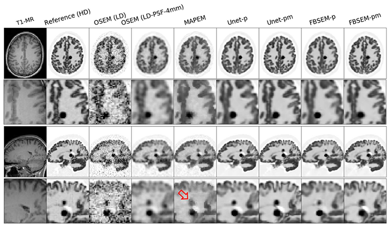
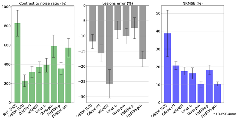
Fig. 3 shows the reconstruction results of a test simulation dataset for different methods considered in this study, from standard OSEM and conventional MAPEM to new DL image denoising and reconstruction methods. Among the methods that only reply on PET data, the results show that both Unet-p and FBSEM-p improve upon the OSEM reconstruction by reducing the noise and contrast to a large extent. For those methods that utilize the additional MR information, Unet-pm and FBSEM-pm both outperform the MAPEM algorithm, which suffers from lack of convergence and suppression of the PET lesions (see the arrow in the coronal view). These results show that Unet-p(m) and FBSEM-p(m) perform similarly on most of the anatomical regions except over the small lesions, as shown in this example test dataset. The performance of the reconstruction methods was the objectively evaluated for all simulation test datasets based on CNR between GM and WM, quantification errors in hot lesions, and NRMSE in the whole brain. As shown in Fig. 4, the Unet-pm and FBSEM-pm show the highest CNR as these methods reduced noise and at the same time improved the convergence. Unet-p showed slightly higher CNR than MAPEM and FBSEM-p, while as could be expected OSEM method achieved the lowest CNR. For hot lesions, the MAPEM and FBSEM-p resulted in the highest (-25.7%) and lowest (-7.4%) quantification errors with respect to reference images. The results show that Unet-pm notably outperformed FBSEM-pm net over the lesions by achieving errors of 10% versus 17.6%. The NRMSE performance of the methods shows that Unet-pm and FBSEM-pm networks result in the lower overall errors.
Fig. 3.
Reconstruction results of a test simulation dataset with two adjacent hot lesions for different reconstruction methods. The arrow shows MAPEM notably suppresses the lesion.
Fig. 4. Quantitative performance of different reconstruction methods averaged on test simulation datasets.
For our simulations, training parameters and schedules chosen according to Table I, these results show that Unet-p outperforms FBSEM-p.
Based on these simulation results, in the training of FBSEM net for in-vivo datasets, as shown in Table I, we increased the number of kernels and reduced its depth (due to GPU memory limitations), which resulted in 1.5 times more trainable parameters compared to simulations. At the same time, we pushed the U-net to its limit of performance, by increasing the number of its kernels (based on the capacity of our GPU memory), resulting in ~5 times more trainable parameters compared to simulations.
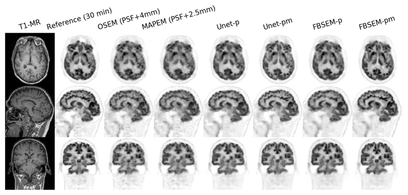
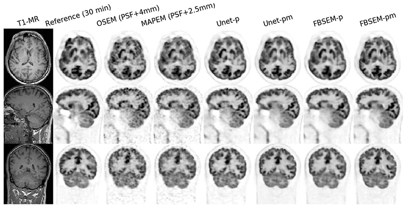
Figs. 5 and 6 compare the reconstruction results of the studied methods for two 2-min in-vivo scans in comparison with their reference 30-min scans (i.e., 15 times longer scan). As shown, the OSEM reconstruction notably suffers from noise, while MAPEM shows the lack of convergence, despite its regularization parameter was chosen fairly low; even after 2.5-mm Gaussian filtering the images show some background noise. The results show that Unet-p and FBSEM-p networks achieve fairly comparable performance. Likewise, Unet-pm and FBSEM-pm networks performed similarly and produced images that are visually close to their reference images.
Fig. 5. Reconstruction results of different methods for a 2-min in-vivo dataset in comparison with their reference 30-min scan.
Fig. 6. Similar to Fig. 5, but for PET data of another subject.
Fig. 7 compares the performance of these methods based on mean FDG uptake in WM, cortical GM, and subcortical GM regions averaged over all in-vivo test datasets. Table II summarizes the error percentage of mean activity in each anatomical region averaged over the test datasets, reporting the mean, SD, and RSS of mean and SD for all regions. As seen in Fig. 7, all methods underestimated the mean activity in cortical and subcortical GM regions, except for the pallidum. For these datasets, FBSEM-p(m) nets achieve the closet mean activity to reference scans in most of the GM regions. The results in Table II show that Unet-p and FBSEM-p both achieve RSS errors of 4.7%, with a slight difference in mean and SD errors, and outperform the OSEM method. Among the methods using MR side information, FBSEM-pm shows the lowest RSS (3.0%) compared to Unet-pm (6.8%) and MAPEM (5.9%).
Fig. 7. Quantitative evaluation of different reconstruction methods in terms of mean activity in different regions of the brain averaged across ten test in-vivo datasets.
Table II. Error Percentage of Mean Activity in Different Regions of in-vivo Datasets Together With the Mean, SD, and RSS of All Regional Errors.
| OSEM | MAPEM | UNET–P | UNET–PM | FBSEM–P | FBSEM–pm | |
|---|---|---|---|---|---|---|
| WHITE MATTER | 3.6 | 2.2 | 1.6 | –3.4 | 3.1 | 2.9 |
| GREY MATTER | –6.6 | –3.5 | –5.0 | –5.3 | 4.0 | –2.1 |
| THALAMUS | –5.9 | 4.0 | –3.7 | –6.5 | –3.3 | 0.0 |
| CAUDATE | –14.8 | –11.6 | –7.6 | –7.8 | –9.4 | –4.4 |
| PUTAMEN | –7.5 | –6.2 | –6.2 | –8.7 | –4.9 | –5.3 |
| PALLIDUM | 5.9 | 4.1 | 0.4 | –9.1 | 0.3 | 0.0 |
| HIPPOCAMPUS | –4.1 | –4.6 | –4.0 | –4.6 | –2.9 | –1.4 |
| MEAN | –4.3 | –3.4 | –3.5 | –6.5 | –3.0 | –1.5 |
| SD | 6.5 | 4.8 | 3.1 | 2.0 | 3.6 | 2.6 |
| RSS | 7.8 | 5.9 | 4.7 | 6.8 | 4.7 | 3.0 |
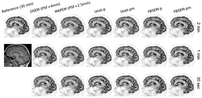
In this work, the DL methods were trained for mapping 2-min data to their reference 30-min data. In order to evaluate their generalization and performance for shorter scan durations, we applied them to an in-vivo dataset with scan durations of 2 min, 1 min, and 30 s (i.e., 15 x, 30 x, and 60 × shorter than their reference scan, respectively). Fig. 8 compares the results for all methods. Note the regularization parameters of the FBSEM-p(m) nets were not modified despite they have been trained for 2-min datasets. Likewise, the regularization parameters of MAPEM for 1-min and 30-s datasets were set to the one chosen for 2-min dataset of this subject. As seen, with shortening scan duration, noise notably dominates OSEM and MAPEM reconstructions. The Unet-p and FBSEM-p both show similar qualitative performance for 2- and 1-min datasets, however for 30-s one, FBSEM-p tends to show less residual noise. For this subject, both Unet-pm and FBSEM-pm nets demonstrate a consistent performance across all three scan durations, which shows their ability to generalize to datasets that they have never been trained for.
Fig. 8.
Real-data performance of the studied methods for reconstruction of reduced scan times (2 min, 1 min, and 30 s) of a subject with respect to their reference 30-min scan. Note the Unet-p(m) and FBSEM-p(m) networks are trained only with scan datasets of 2-min duration.
IV. Discussion
In this study, we applied a proximal splitting technique for MAPEM reconstruction. For a specific regularization parameter (β) and step size (γ), the resulting optimization algorithm reduces to De Pierro’s MAPEM algorithm which is known to be monotonically convergent. However similar to Green’s one-step-late algorithm [26], for an arbitrarily large 3, this algorithm may not converge to a global maximum. A possible solution could be imposing a non-negativity constraint on (7). In fact, as shown in Fig. 1, the residual learning unit (RLU) used in our FBSEM net applies a ReLU activation function to the sum of the input image and the output of the CNN layers in order to explicitly ensure the non-negativity of the output. Moreover, our proposed FBSEM algorithm makes use of oS for acceleration which is known to cycle over a number of image estimates, especially for unbalanced subsets. A possible solution is to upgrade the oSEM update in (8) by a row-action maximum-likelihood algorithm (RAMLA) [27], which is a convergent oS algorithm. Moreover, since the FBSEM algorithm is based on an optimization transfer approach, convergence can be slow. In this study, we used a CNN-based prior for regularization in the FBSEM net. Depending on whether the learned prior is convex or not, the trained FBSEM net can be convergent (if N sub = 1) or nonconvergent. The convexity of the learned priors which do not have an explicit functional form can potentially be tested using nonparametric techniques [28], which is behind the scope of this article.
Our proposed reconstruction network has a number of advantages. Compared to the recently proposed BCD net [17] or EM net [29], which alternate between an MLEM reconstruction and a CNN-based image denoising module, model parameters in FBSEM net are shared across all reconstruction states (similar to RNNs), while BCD and EM nets employ separate networks for each reconstruction states. Sharing model parameters not only notably reduces the number of trainable parameters but also allows the trained network to be used with a different number of iterations during inference [22]. Unlike BCD net and Gong et al. [13], the regularization (penalty) parameter is learned from the data and the network can be initialized with a uniform image estimate. Unlike EM net and similar to BCD net, the data-fidelity-based EM update and the CNN-based regularization operations are performed in parallel in our network, and during training, the backpropagation was set to pass only through the regularization and fusion steps eliminating the need for computationally intensive differentiation of PET forward and backward projections. In addition, our proposed network operates in PET-only and PET-MR modes.
Following the proposal and implementation of the FBSEM net, which can potentially improve upon prior networks owning to the above advantages, our next goal was to compare its performance with the best of post-reconstruction DL-based denoising. In this work, U-Net was chosen as a widely used encoder-decoder CNN. Lu et al. [30] recently showed that an optimized 3-D U-Net could outperform a convolutional autoencoder network and a generative adversarial net for lung nodule quantification in reduced dose scans. our results in Fig. 4 showed that Unet-p(m) net has a relatively comparable performance to FBSEM-p(m) net, even in its PET-MR mode, Unet-pm outperformed FBSEM-pm in preserving PET lesions in our simulations, despite their NRMSE over whole brain was comparable. This can be attributed to the fact that U-Net extracts and captures features at a multiresolution level, and that the employed Unet-pm in our simulations has ~200 times more trainable parameters that the FBSEM-pm net. For in-vivo datasets, we increased the number of convolution kernels and decreased the number of reconstruction states and learning rate of FBSEM-p(m) net. At the same time, we increased the number of kernels for Unet-p(m) nets to potentially improve its performance even further, which resulted in ~600 times more trainable parameters compared to FBSEM nets. The in-vivo results showed that FBSEM-p and Unet-p perform comparatively for the PET mode, however for the PET-MR mode, FBSEM-pm outperforms Unet-pm on average.
The results in Fig. 4 have been averaged across ten test datasets; since the reference HD images have fairly low noise (see Figs. 2 and 3), the variability of CNR for HD images represents the fact that our phantoms were generated from MR images of patients suspected of epilepsy and dementia, for which there may be cortical atrophy and partial volume effects of differing degrees. The results in Fig. 4 show that the networks that used MR images (i.e., FBSEM-pm and Unet-pm) are able to capture that variability to some extent despite their mean CNRs being notably lower.
Similar to the EM net, a residual U-Net could be used as the regularization module in the FBSEM net. However, since U-Net usually employs a large number of trainable parameters the training of the resulting FBSEM network would be tremendously memory demanding. Note that the inference of FBSEM net or generally any network is notably less memory demanding, as automatic differentiation (autograd) will be inactive and hence tensors’ gradient will not be tracked and stored in memory. Our initial 2-D simulation results presented in [25] showed that FBSEM net with the smaller RLU architecture achieves a comparable performance to when a residual U-Net is used inside FBSEM net. Hence, in this study, we opted for the less memory demanding RLU network, on the understanding that the FBSEM net results would be representative also of the case of when a U-Net is used instead of an RLU. Furthermore, our previous 2-D results showed that post-reconstruction denoising using a U-Net outperforms an RLU. Therefore, given these initial results, and furthermore also those reported in the literature (e.g., [30]), we chose a U-Net to best represent the performance of post-reconstruction denoising networks, just as using an RLU in FBSEM net best represents its performance as well.
The number of parameters in our U-Net trained for in-vivo datasets is nearly 48M parameters, which is in the range used in modern CNNs; from ~40M in Inception-v4 to ~140M in the VGG net. However, for a fixed amount of training data, the large number of parameters can increase the chance of overfitting and generalization error. In Fig. 8, we used the models trained on only 2-min data for testing on even shorter scans, to assess performance on a domain different to that of the training data. Given that the Unet-p model achieves a comparable performance to FBSEM-p for a 2-min test dataset and that these models have not been trained for 1-min and 30-s scans, the slightly poorer performance of the Unet-p for 30-s scan should not be interpreted as overfitting but better domain adaptation capabilities of the FBSEM net. This can be attributed to the fact that noise is iteratively amplified during OSEM reconstruction, whereas the FBSEM net can suppress the noise from the early stages.
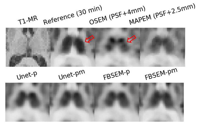
In this work, we considered DL image enhancement and reconstruction of reduced-duration and full-dose scans instead of reduced-dose and full-duration ones. Because we believe the immediate clinical test of DL methods will be for reduced duration studies as they can be done retrospectively and will have less complications for ethics approval compared to reduced dose studies which are prospective and require modification to clinical acquisition protocols. Hence, in this study, the 30-min list-mode FDG data were resampled to emulate 2-min scans and DL networks were trained to reduce noise in the 2-min PET images and improve their image quality toward their reference 30-min images. However, since a 15 × scan-time reduction was considered in order to make noise vividly dominant, there is a chance for physiological mismatches between the two scans over brain regions with rapid/delayed glucose metabolism in some patients. For these cases, the DL networks will not only reduce noise but also predict what the physiology of those regions could be if the scan time had been prolonged for another 28 min. Fig. 9 illustrates this for the thalamus in a subject. As shown, there is a physiology mismatch between thalamus’ uptake after 2- and 30-min scans. MAPEM reconstruction flattens uptake in the thalamus by reducing noise or PSF artifacts, but the DL methods not only flatten the uptake but also increase it toward its reference 30-min uptake. Another physiology mismatch can be seen in Fig. 6, a sagittal view, where the tracer’s uptake has been washed out in the caudate during the 30-min course of scan compared the 2-min scan. As seen in the transverse view, this patient has hypometabolism in their right hemisphere. It should be noted that for whole-body scans with 3-4 min acquisition per bed, scan-time reductions up to 4 will make noise vividly dominant, hence the chance of physiology changes will be relatively lower.
Fig. 9.
Physiology mismatches in thalamus between a reference 30-min scan and a 2-min scan (obtained by the replay of 30-min list-mode data). DL methods (second row) have increased the thalamus’ 2-min uptake toward its 30-min reference uptake.
In our FBSEM networks, the number of kernels of all D layers is the same. As summarized in Table I, for in-vivo datasets, we chose a taller and shallower network (37 kernels and 3 layers) whereas for simulated datasets, we chose a shorter and deeper one (16 kernels and 9 layers). The reason is that our simulations in Fig. 4 showed that the FBSEM-p(m) nets are not quantitatively as good as the Unet-p(m) networks. Given that these networks operate on 3-D images, our intuition was that the 16 kernels in the first layer of an FBSEM net might not be sufficient to capture 3-D edges, hence we opted for a taller network at the compromise of making the network shallower due to GPU memory limitations. Since our simulations were made as realistic as possible, the improved quantitative performance of the FBSEM nets for in-vivo datasets compared to simulations implies that our intuition might be correct. In general, for a specific DL task, a network’s hyperparameters can be chosen based on the network’s performance on validation datasets. As mentioned earlier, we could not afford the computational load of the validation process, nonetheless, our results for unseen test datasets were acceptable. Had we included the validation; the FBSEM net’s performance could have been potentially even better.
The in-vivo brain PET and MR images are often well aligned, nonetheless, there is a chance of head drift between the different PET and MR acquisition time windows, therefore in this study, we assured their alignment using SPM co-registration. In regard to misalignments, our simulation results with lesion mismatches between PET and MR showed that Unet-pm and FBSEM-pm nets outperformed the conventional Bowsher MAPEM algorithm in lesion quantification, which indicates the potential ability of DL methods in dealing with mismatches. This can be investigated in a future work. Future work would also include evaluation of the number of reconstruction states and depth of the FBSEM net on its performance and investigation of memory-efficient reconstruction algorithms and strategies to train a fully unrolled FBSEM net for 3-D whole-body PET-MR image reconstruction.
V. Conclusion
A model-based DL reconstruction network was designed by unrolling an optimization algorithm that we proposed in this study for MAPEM image reconstruction. The proposed FBSEM net was evaluated in PET-only and PET-MR modes in comparison with the state-of-the-art U-Net denoising and conventional MR-guided MAPEM and standard OSEM methods. our simulation and in-vivo results showed that both DL-based techniques outperform the conventional methods. It was found that for the chosen network parameters and training schedules the Unet-p and FBSEM-p net achieve a fairly comparable performance for both simulation and in-vivo datasets. For simulations, Unet-pm net showed lower quantification errors for PET unique lesions while achieving a similar NRMSE to FBSEM-pm net, whereas for in-vivo datasets, the FBSEM-pm outperformed Unet-pm and achieved the lowest quantification error amongst all reconstruction methods. It can be concluded that DL-based post-reconstruction denoising methods can potentially perform as good as DL-based reconstruction methods.
Acknowledgements
The authors would like to thank Prof. Alexander Hammers and Dr. Colm McGinnity from King’s College London and Guy’s and St. Thomas’ PET Centre for providing the clinical brain PET-MR datasets. For reproducible research and compliance with EPSRC’s policy framework on research data, PyTorch codes, and simulation datasets for the training of a 2-D FBSEM net will be openly available at https://github.com/Abolfazl-Mehranian/FBSEM/.
This work was supported in part by the Engineering and Physical Sciences Research Council (EPSRC) under Grant EP/M020142/1; in part by the Wellcome EPSRC Centre for Medical Engineering at King’s College London under Grant WT 203148/Z/16/Z; and in part by the Department of Health through the National Institute for Health Research (NIHR) comprehensive Biomedical Research Centre award to Guy’s & St. Thomas’ NHS Foundation Trust in partnership with King’s College London and King’s College Hospital NHS Foundation Trust.
Footnotes
see Acknowledgment for the source code.
References
- [1].Qi J, Leahy RM. Iterative reconstruction techniques in emission computed tomography. Phys Med Biol. 2006 Aug;51(15):R541–R578. doi: 10.1088/0031-9155/51/15/R01. [DOI] [PubMed] [Google Scholar]
- [2].Bai B, Li Q, Leahy RM. Magnetic resonance-guided positron emission tomography image reconstruction. Seminars Nucl Med. 2013;43(1):30–44. doi: 10.1053/j.semnuclmed.2012.08.006. [DOI] [PMC free article] [PubMed] [Google Scholar]
- [3].Mehranian A, et al. PET image reconstruction using multiparametric anato-functional priors. Phys Med Biol. 2017 Jul;62(15):5975–6007. doi: 10.1088/1361-6560/aa7670. [DOI] [PubMed] [Google Scholar]
- [4].Bland J, Belzunce MA, Ellis S, McGinnity CJ, Hammers A, Reader AJ. Spatially compact MR-guided kernel EM for PET image reconstruction. IEEE Trans Radiat Plasma Med Sci. 2018 Sep;2(5):470–482. doi: 10.1109/TRPMS.2018.2844559. [DOI] [PMC free article] [PubMed] [Google Scholar]
- [5].Bland J, et al. MR-guided kernel EM reconstruction for reduced dose PET imaging. IEEE Trans Radiat Plasma Med Sci. 2018 May;2(3):235–243. doi: 10.1109/TRPMS.2017.2771490. [DOI] [PMC free article] [PubMed] [Google Scholar]
- [6].Wang G, Ye JC, Mueller K, Fessler JA. Image reconstruction is a new frontier of machine learning. IEEE Trans Med Imag. 2018 Jun;37(6):1289–1296. doi: 10.1109/TMI.2018.2833635. [DOI] [PubMed] [Google Scholar]
- [7].Gong K, Berg E, Cherry SR, Qi J. Machine learning in PET: From photon detection to quantitative image reconstruction. Proc IEEE. 2020 Jan;108(1):51–68. doi: 10.1109/JPROC.2019.2936809. [DOI] [PMC free article] [PubMed] [Google Scholar]
- [8].Zhu B, Liu JZ, Cauley SF, Rosen BR, Rosen MS. Image reconstruction by domain-transform manifold learning. Nature. 2018 Mar;555(7697):487–492. doi: 10.1038/nature25988. [DOI] [PubMed] [Google Scholar]
- [9].Haggstrom I, Schmidtlein CR, Campanella G, Fuchs TJ. DeepPET: A deep encoder-decoder network for directly solving the PET image reconstruction inverse problem. Med Image Anal. 2019 May;54:253–262. doi: 10.1016/j.media.2019.03.013. [DOI] [PMC free article] [PubMed] [Google Scholar]
- [10].Gong K, Guan JH, Liu CC, Qi JY. PET image denoising using a deep neural network through fine tuning. IEEE Trans Radiat Plasma Med Sci. 2019 Mar;3(2):153–161. doi: 10.1109/Trpms.2018.2877644. [DOI] [PMC free article] [PubMed] [Google Scholar]
- [11].Liu CC, Qi J. Higher SNR PET image prediction using a deep learning model and MRI image. Phys Med Biol. 2019 May;64(11) doi: 10.1088/1361-6560/ab0dc0. Art. no. 115004. [DOI] [PMC free article] [PubMed] [Google Scholar]
- [12].Cheng L, Ahn S, Ross S, Qian H, De Man B. Accelerated iterative image reconstruction using a deep learning based leapfrogging strategy. Proc Fully Three-Dimensional Image Reconstruct Radiol Nucl Med (Fully3D) 2017:715–720. [Google Scholar]
- [13].Gong K, et al. Iterative PET image reconstruction using convolutional neural network representation. IEEE Trans Med Imag. 2019 Mar;38(3):675–685. doi: 10.1109/Tmi.2018.2869871. [DOI] [PMC free article] [PubMed] [Google Scholar]
- [14].Ronneberger O, Fischer P, Brox T. U-Net: Convolutional networks for biomedical image segmentation. In: Navab N, Hornegger J, Wells WM, Frangi AF, editors. Medical Image Computing and Computer-Assisted Intervention MICCAI 2015. Springer; Cham, Switzerland: 2015. pp. 234–241. [Google Scholar]
- [15].Gong K, Catana C, Qi J, Li Q. PET image reconstruction using deep image prior. IEEE Trans Med Imag. 2019 Jul;38(7):1655–1665. doi: 10.1109/TMI.2018.2888491. [DOI] [PMC free article] [PubMed] [Google Scholar]
- [16].Cui J, et al. PET image denoising using unsupervised deep learning. Eur J Nucl Med Mol Imag. 2019 Dec;46(13):2780–2789. doi: 10.1007/s00259-019-04468-4. [DOI] [PMC free article] [PubMed] [Google Scholar]
- [17].Lim H, Huang Z, Fessler JA, Dewaraja YK, Chun IY. Application of trained deep BCD-Net to iterative low-count PET image reconstruction; Proc IEEE Nucl Sci Symp Med Imag Conf (NSS/MIC); Sydney, NSW, Australia. 2018. Nov, pp. 1–4. [DOI] [Google Scholar]
- [18].Wang G, Qi J. Penalized likelihood PET image reconstruction using patch-based edge-preserving regularization. IEEE Trans Med Imag. 2012 Dec;31(12):2194–2204. doi: 10.1109/TMI.2012.2211378. [DOI] [PMC free article] [PubMed] [Google Scholar]
- [19].Combettes PL, Pesquet J-C. Proximal splitting methods in signal processing. In: Bauschke HH, Burachik RS, Combettes PL, Elser V, Luke DR, Wolkowicz H, editors. Fixed-Point Algorithms for Inverse Problems in Science and Engineering. Springer; New York, NY, USA: 2011. pp. 185–212. [Google Scholar]
- [20].De Pierro AR. On the relation between the ISRA and the EM algorithm for positron emission tomography. IEEE Trans Med Imag. 1993 Jun;12(2):328–333. doi: 10.1109/42.232263. [DOI] [PubMed] [Google Scholar]
- [21].Levitan E, Herman GT. A maximum a posteriori probability expectation maximization algorithm for image reconstruction in emission tomography. IEEE Trans Med Imag. 1987 Sep;6(3):185–192. doi: 10.1109/TMI.1987.4307826. [DOI] [PubMed] [Google Scholar]
- [22].Aggarwal HK, Mani MP, Jacob M. MoDL: Model-based deep learning architecture for inverse problems. IEEE Trans Med Imag. 2019 Feb;38(2):394–405. doi: 10.1109/TMI.2018.2865356. [DOI] [PMC free article] [PubMed] [Google Scholar]
- [23].He K, Zhang X, Ren S, Sun J. Deep residual learning for image recognition; Proc IEEE Conf Comput Vis Pattern Recognit (CVPR); Las Vegas, NV, USA. 2016. Jun, pp. 770–778. [DOI] [Google Scholar]
- [24].Bowsher JE, et al. Utilizing MRI information to estimate F18-FDG distributions in rat flank tumors; Proc IEEE Symp Conf Rec Nucl Sci; Rome, Italy. 2004. Oct, pp. 2488–2492. [DOI] [Google Scholar]
- [25].Mehranian A, Reader AJ. Model-based deep learning PET image reconstruction using forward-backward splitting expectation maximisation; presented at the IEEE Nucl Sci Symp Med Imag Conf (NSS/MIC); Manchester, U.K. 2020. pp. 1–4. [DOI] [PMC free article] [PubMed] [Google Scholar]
- [26].Green PJ. On use of the EM algorithm for penalized likelihood estimation. J Roy Stat Soc Series B. 1990;52(3):443–452. doi: 10.1111/j.2517-6161.1990.tb01798.x. [DOI] [Google Scholar]
- [27].Browne J, Pierro ABD. A row-action alternative to the EM algorithm for maximizing likelihood in emission tomography. IEEE Trans Med Imag. 1996 Oct;15(5):687–699. doi: 10.1109/42.538946. [DOI] [PubMed] [Google Scholar]
- [28].Juditsky A, Nemirovski A. On nonparametric tests of positivity/monotonicity/convexity. Ann Stat. 2002 Jan;30:498–527. doi: 10.1214/aos/1021379863. [DOI] [Google Scholar]
- [29].Gong K, et al. EMnet: An unrolled deep neural network for PET image reconstruction. Proc Med Imaging Phys Med Imaging. 2019 Mar; doi: 10.1117/12.2513096. Art. no. 1094853 [Online]. Available. [DOI] [Google Scholar]
- [30].Lu W, et al. An investigation of quantitative accuracy for deep learning based denoising in oncological PET. Phys Med Biol. 2019 Aug;64(16) doi: 10.1088/1361-6560/ab3242. Art. no. 165019. [DOI] [PubMed] [Google Scholar]


