Abstract
The purpose of this study is to enable high spatial resolution voxelwise quantitative analysis of myocardial perfusion in dynamic contrast-enhanced cardiovascular MR, in particular by finding the most favorable quantification algorithm in this context. Four deconvolution algorithms—Fermi function modeling, deconvolution using B-spline basis, deconvolution using exponential basis, and autoregressive moving average modeling —were tested to calculate voxel-wise perfusion estimates. The algorithms were developed on synthetic data and validated against a true gold-standard using a hardware perfusion phantom. The accuracy of each method was assessed for different levels of spatial averaging and perfusion rate. Finally, voxel-wise analysis was used to generate high resolution perfusion maps on real data acquired from five patients with suspected coronary artery disease and two healthy volunteers. On both synthetic and perfusion phantom data, the B-spline method had the highest error in estimation of myocardial blood flow. The autoregressive moving average modeling and exponential methods gave accurate estimates of myocardial blood flow. The Fermi model was the most robust method to noise. Both simulations and maps in the patients and hardware phantom showed that voxel-wise quantification of myocardium perfusion is feasible and can be used to detect abnormal regions. Magn Reson Med 68:1994-2004, 2012. © 2012 Wiley Periodicals, Inc.
Keywords: myocardial perfusion, voxel-wise quantification, accuracy, noise robustness
Introduction
Detection of myocardial ischemia is the key to the diagnosis of coronary artery disease (1). Several invasive techniques, including Doppler catheterization and coronary sinus thermo dilution, are available for measuring myocardial blood flow (MBF) in humans. These methods, which are variations of indicator dilution methods, are invasive and can only assess average perfusion of whole coronary artery territories. Amongst noninvasive imaging techniques, positron emission tomography (PET) is currently regarded as a gold standard for the quantification of absolute MBF. However, this technique has several drawbacks including low spatial resolution (making it unsuitable for the detection of subtle subendocardial perfusion defects), patient radiation exposure, and high cost (2,3).
Compared with PET, dynamic contrast-enhanced cardiovascular magnetic resonance (DCE-CMR) imaging has several potential advantages: superior spatial resolution, absence of ionizing radiation, and availability of stable and inert contrast agents of low toxicity. Estimation of MBF from DCE-CMR studies has been reported using a number of different analysis techniques including quantitative and semiquantitative methods (4–14).
Although favorable results with semiquantitative techniques such as upslope analysis of the myocardial time-intensity curve have been reported, these methods have shown to underestimate the perfusion parameters (15,16). Moreover, semiquantitative analysis relies on a ratio which introduce a bias on the data itself and the relationship between MBF and the semiquantitative methods parameters such as the curve upslope is not as clear-cut as the relationship between MBF and the impulse response amplitude which we get from quantitative analysis (8,17), whereas using fully quantitative analysis allows the absolute quantification of MBF in units of ml/g/min and may permit more accurate and objective assessment of altered myocardial perfusion in patients with heart disease.
Quantitative methods can be further divided into two groups: model-based and model-independent analysis.
Model-independent quantitative analysis, based on the central volume principle established by Zierler et al.(18), has been applied to DCE-CMR acquired data to determine myocardial perfusion (4–7,10,13). It is widely used with intravascular contrast agents and has been applied with extracellular contrast agents to quantify renal and tumor perfusion (11,19,20).
Model independent methods require that the measured blood, C aif(t) and tissue, C myo(t), enhancement data, which are related together through the following equation:
| [1] |
are mathematically deconvolved to estimate tissue impulse response function, h(t). The maximum amplitude of h(t) is directly related to the rate of perfusion (4,5,7,10,18), independent of biological parameters such as the distribution and permeability of the vessels within the tissue via:
where dt is the sampling rate of perfusion images and SGmyo is the myocardial density, which was assumed to be equal to 1.05 g/mL (18,21).
This task is challenging because it amounts to inverting the convolution of h(t) with C aif(t), which is in this context an ill-posed noise sensitive inverse problem and needs regularization (22,23).
To the best of our knowledge, myocardial perfusion estimates have only been calculated for segmental quantification of myocardial perfusion, i.e., time curves averaged over groups of voxels, while voxel-wise analysis, although previously used on an experimental isolated pig heart model (10), has not been developed for clinical practice.
Voxel-wise myocardium perfusion analysis allows the quantification of MBF with the potential to preserve the information about extension, localization, and transmurality of ischemia. This technique produces higher resolution images of MBF and thus has the potential to allow a more accurate diagnosis of coronary artery disease. However, the lower contrast to noise ratio (CNR) of single voxel curves may reduce the accuracy and reliability of the measurement.
The objective of this study is to demonstrate the feasibility and validation of voxel-wise perfusion analysis on high-resolution k-t perfusion data, by comparing the main regularized deconvolution methods in terms of accuracy and robustness to noise.
Theory
Although many regularization methods have been used for deconvolution, the most popular methods for kernel estimation in DCE-CMR include: Fermi function modeling (6,24), deconvolution using a B-spline basis (5,7), and deconvolution using an exponential approximation (11). More recently, autoregressive moving average (ARMA) has also been used to measure the tissue impulse response (10,25).
Fermi Function Modeling
The use of the Fermi function was motivated by the observed similarity between the simulated impulse response for an intravascular tracer and the shape of the Fermi function. Jerosch-Herold et al. (6) and Wilke et al. (24) fitted time curves for the tissue impulse response function, h(t), to the Fermi function with the following analytical expression:
| [2] |
using a Marquardt-Levenberg nonlinear least square algorithm by letting k, R and τ0 vary and keeping τd fixed. In Eq. 2, u(t — τd) is the unit step function, τd accounts for the delay time between the appearance of the signal in the LV blood pool and myocardial region of interest (ROI) and τ0 characterizes the width of the shoulder of the Fermi function during which little or no contrast agent has left ROI. R is the index of contrast agent influx parameter, and k represents the decay rate of h(t) due to contrast agent wash out. From Eq. 2, MBF is calculated as h(t) at t = 0.
Deconvolution Using B-Spline Basis
Jerosch-Herold et.al (7) developed a model-independent deconvolution method that parameterized h(t) as a sum of weighted B-spline functions and stabilized the solution by using Tikhonov regularization. In the above sum, represents the jth B-spline of order k (7,26).
All previous studies that have used this method (4,5,7,8) have found the tissue impulse response by using the following least square minimization problem and Tikhonov regularization:
| [3] |
where ▽ represents the temporal difference operator, λ is a regularization parameter, and ||·|| denotes the Euclidean norm. Using L-curve analysis or generalized crossvalidation, will lead to a good choice of (27). Singular value decomposition can be used to obtain a stable solution for this ill-posed least square minimization problem.
Exponential Basis Deconvolution
Recently, Keeling et al.(11) developed a model-independent deconvolution method using an approximation basis of exponential functions constrained to be non-negative and non-increasing for the tissue impulse response and demonstrated that this method compares favorably to the standard singular value decomposition method in brain perfusion imaging (11,20). Exponential basis deconvolution regularizes naturally by constraining the estimated kernel to be monotonic.
In addition to the choice of approximation basis, further regularization is implemented in terms of the number of base functions (M) and the distribution of their parameters (11).
Finally, h(t) is found by using the following linearly constrained least squares problem:
| [4] |
Auto Regressive Moving Average
Autoregressive moving average (ARMA) models are mathematical models of the persistence, or autocorrelation, in a time series. The ARMA model assumes that the discrete time samples of measured C myo(t) and C aif(t) are related together according to:
| [5] |
To identify the aj and the bi, the above equation can be written for t = 1 … N
| [6] |
where N represents the number of acquisition data points and assuming null initial condition. The least squares solution of Eq. 6, after choosing the best value for L and Q which reduces the degree of freedom of the deconvolution equation and make it more stable, gives the coefficients aj, bi and hence h(t) can be computed by finding the solution of Eq. 5 to the Dirac function (δ(t = 1) if t = 0 and zero if t ≠ 0) (10,25).
Estimation of the ARMA model order requires that the model to be fitted for many L and Q orders to find the smallest values of L and Q which provide an acceptable fit to the data and reduce the computational burden. A study has been done on the ARMA model to obtain the best order for perfusion quantification previously (25).
Finding appropriate orders for the ARMA model can be facilitated by plotting the partial autocorrelation functions for an estimate of L and similarly using the autocorrelation functions for an estimate of Q (28,29). Note that the ARMA approach is also justified from the physiological perspective, as it is a discrete-time version of perfusion modeling using linear differential equations with constant coefficients (25,30).
Material and Methods
Synthetic Data
A first experiment was performed by using simulated data with known perfusion values and by calculating the absolute error of quantification.
This experiment was undertaken to verify the reliability of the perfusion estimates at different simulated levels of CNR and flow for each quantification method.
Noiseless gold standard tissue impulse response, h GS(t), were constructed by using the following phar-maco-kinetic model, described by Lindsey et al. (30):
| [8] |
where u(t) is the unit step function.
The physiological parameters, i.e., λ n, n = 1,2,3, were chosen to generate tissue responses of the same order as those obtained by the fitting of real series of DCE-CMR acquisitions. λ2 and λ3 have been kept fixed on 0.21 and 0.36, respectively, and the λ1 value has been changed to simulate a series of perfusion values between 0.5 and 5 mL/g/min. Table 1 represents the chosen λ1 values for each simulated MBF level.
Table 1. λi Values for Generating Synthetic Data.
| Simulated Flow (mL/g/min) | λ 1 |
|---|---|
| 0.5 | 1.5 |
| 1 | 2.4 |
| 1.5 | 2.85 |
| 2 | 3.2 |
| 2.5 | 3.5 |
| 3 | 3.68 |
| 3.5 | 3.79 |
| 4 | 3.94 |
| 4.5 | 4.06 |
| 5 | 4.16 |
C aif(t) used in this experiment is a convolution of many exponentials as suggested in (11) to model the propagation of an impulsive bolus injection through several compartments of the cardiovascular system. The injected bolus typically travels through at least three major compartments: from the injection site through the right heart, from the right heart through the lungs to the left heart, and finally from the left heart to the myocardium tissue. For simplicity, we assumed same mean transit time (1/v > 0, v = 0.3897), and thus the same compartment kernel ve-vt for all compartments. As a result, the arterial input at the tissue site can be formulated as n (n = 4) convolution of the unit kernel:
Initial C myo(t) was then obtained by convolving hGS(t) with the simulated C aif(t) (11). Rician noise of variable amplitudes were added to both C aif(t) and C myo(t) (31,32). The range of noise amplitude was chosen so that CNR in the both C aif(t) and C myo(t) would be between 1 and 40. Equal noise amplitudes were added to both C aif(t) C myo(t) at each CNR level. CNR is defined as the ratio of the signal change from baseline to peak of enhancement data, divided by the standard deviation (STD) of the signal intensity curves before contrast.
MRI Image Acquisition
All data (phantom and patient) were acquired on a Philips Achieva 3T (TX) system, equipped with a 32-channel cardiac phased array receiver coil (Philips Health Care, Best, Netherlands).
To avoid any confounding effects due to signal saturation, a universal dual-bolus injection scheme was performed in patients and the perfusion phantom as described by Ishida et al. (33). We used 0.001 mEq/kg of body weight as a prebolus and 0.01 mEq/kg of body weight as bolus (Gadobutrol Gadovist®, Bayer Schering, Germany). The boluses were injected at 4 mL/s followed by a 20 mL saline flush.
Hardware Perfusion Phantom
A second experiment was performed on a hardware perfusion phantom, which was recently developed by our group (34).The perfusion phantom resembles the anatomy of a 60 kg patient. It allows an efficient and reproducible simulation of myocardial perfusion acquisition, providing data suitable for quantification and with the possibility of a validation of the perfusion quantification results with a true gold standard.
Phantom data were acquired in one slice in a transverse geometry, visualizing the progression of the bolus of contrast agent in the large thoracic vessels and the myocardial compartments in the same image, with a saturation recovery gradient echo method (repetition time/ echo time 3.0 ms/1.0 ms, flip angle 15°; effective k-t SENSE acceleration 3.8 fold, spatial resolution 1.2 x 1.2 x 10 mm3, saturation delay 120 ms, Matrix size 132 x 132, BW 2137 Hz, FOV 24 x 24) (35–37).
Myocardial perfusion was simulated for the following experimental conditions. The perfusion phantom has two compartments. Average flow in the reference compartment was kept constant at perfusion rate equal to 5 mL/g/min. Average perfusion rate in the variable compartment ranging across the following values: 1, 2, 3, 4, and 5 mL/g/min. CNR was manipulated by varying the distance of the anterior surface coil from the phantom (high-CNR acquisitions with the coil as close as possible to the phantom; low-CNR acquisitions with the coil 10 cm from the phantom).
Patient Study
In this study, we present preliminary data obtained for voxel-wise quantification of DCE-CMR data from five patients with angina symptoms referred to evaluate the presence and extension of inducible abnormalities of MBF during stress with adenosine and two healthy volunteers. The study was prospectively performed at Guy’s and St Thomas’ Hospital London (UK). The institutional review board approved the study, and all patients signed an informed consent to be included.
Aim of perfusion study was to prove the feasibility of the perfusion maps in patients with coronary artery disease and in volunteers.
Patients perfusion data were acquired in three slices (apical, mid cavity, and basal) in a short axis geometry, visualizing the progression of the bolus of contrast agent in the large thoracic vessels and the myocardial compartments in the same image, with a saturation recovery gradient echo method (repetition time/echo time 3.0 ms/1.0 ms, flip angle 15°; effective k-t SENSE acceleration 3.8 fold, spatial resolution 1.2 x 1.2 x 10 mm3, saturation delay 120 ms, Matrix size 251 x 251, BW 724 Hz, FOV 31 x 31) (35–37).
MR Image Processing
Accurate voxel-based MBF estimation requires respiratory motion correction and myocardial contour delineation. We developed an automated approach based on (38,39) in which respiratory motion was removed using affine image registration by maximization of the joint correlation between consecutive dynamics within an automatically determined ROI. Then, a temporal maximum intensity projection was calculated to serve as a feature image for an automatic contour delineation method based on active contour models (38,39). Signal intensities were then sampled using bilinear interpolation at a grid of 60 angular positions and 10 transmural positions (or layers). The transmural positions were located on chords perpendicular to the myocardial centre-line.
To maximize reproducibility of MBF quantification, care was taken to obtain C aif(t) in a robust and reproducible way. C aif(t) was obtained by sampling the trimmed median intensity within a ROI in the blood pool of the basal slice. To be robust against the present of papillary muscles, the ROI was obtained by down scaling the endocardium contours. Furthermore, the trimmed median operator ignores 15% of outlier samples. The resulting signal is smooth and represents the AIF closest to the Ostia, (the true location of the input to the coronary system). Before deconvolution analysis, baseline correction that includes scaling of the signal intensities proportional to coil sensitivity and correcting for an offset to shift the baseline signal to zero has been performed. Moreover, spatial filtering, gaussian filter of size 5, and temporal filtering, a 30th order Hamming-window based low pass finite impulse response filter with normalized cut-off frequency of 0.23 (40), were performed on the extracted signal intensity curves. For all models, the perfusion estimates were computed by deconvolving the measured blood and tissue enhancement data during the first pass of contrast agent in myocardium.
The constrained least square problems were solved using lsqlin for Eq. 3, Eq. 4, and Eq. 6 and lsqnonlin for Eq. 2 in MATLAB(Mathworks, Natick, Massachusetts, USA, version R2010b) (11,22). We used fourth-degree B-spline polynomial with 15 equally spaced break points (7) and 10 time scale (M = 10) for exponential bases deconvolution (11) for the representation of impulse response in this study. To render the deconvolution process more stable and reduce the computational burden, second-order autoregressive model, i.e., ARMA (Q = 0,L = 2), (25), was chosen for quantification.
Statistical Analysis
In synthetic numerical and hardware perfusion phantom experiments, considered methods were compared by using the curve fit relative error:
| [9] |
and absolute perfusion error (e a), which is defined when the reference perfusion value, MBFGS is available as:
Mean ± STD of ea was calculated for each different condition tested in the perfusion phantom and synthetic data.
Results
Synthetic Data
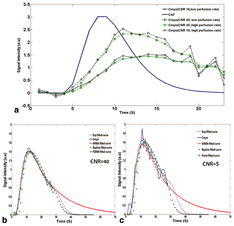
Figure 1a shows plots of simulated C aif(t) and C myo(t) curves for different level of CNR and perfusion rates. C myo for a synthetic myocardium voxel along with the estimated C myo curves, which have been obtained using ARMA, exponential, B-spline, and Fermi method, at CNR = 40 and CNR = 5 are shown in Fig. 1b and c, respectively.
Fig. 1.
In a, the synthetic input and output signal intensity (in arbitrary units: a.u.) curves at high simulated perfusion rate and low simulated perfusion rate at different CNR levels. The solid line corresponds to the synthetic C aif(t), and the dotted lines correspond to synthetic C myo(t). In b and c, C myo(t) for a synthetic myocardium voxel along with the estimated curves using ARMA, exponential, B-spline, and Fermi method are shown at CNR = 40 and CNR = 5 (MBFGS = 1 mL/g/min), respectively. In general, all methods give good results in terms of fit (x < 0.9% for high CNR; x < 2% for low CNR). [Color figure can be viewed in the online issue, which is available at wileyonlinelibrary.com.]
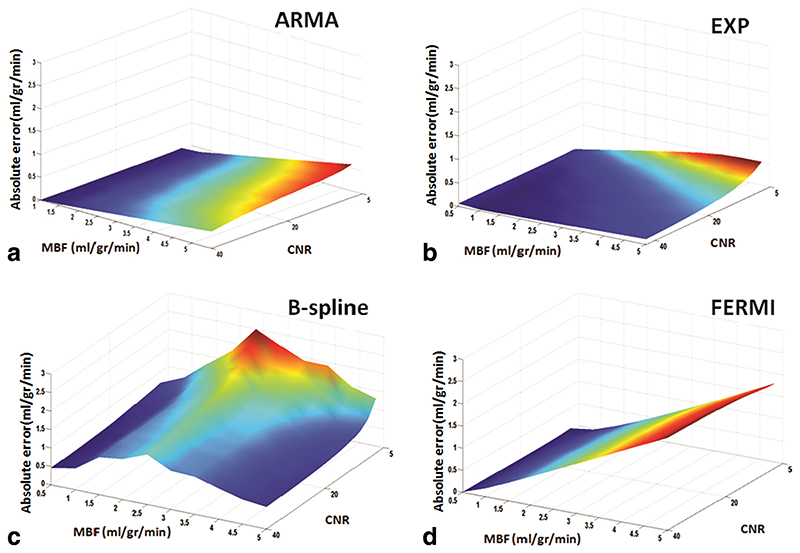
Figure 2 shows the absolute errors (e a) of the synthetic data MBF estimates obtained with the four methods— ARMA (a), exponential (b), B-spline (c), and Fermi (d)— at different levels of flow and CNR. e a is averaged over all voxels at each CNR level and perfusion rate.
Fig. 2.
Surface plot of simulated flow rates (0.5 to 5 mL/g/min) absolute error (e a) at different CNR levels (5 to 40 with 15 steps) for the ARMA, exponential, B-spline, and Fermi model is represented in figures a, b, c, and d, respectively. ea is averaged over all voxels at each flow and CNR level. In general, the ARMA and the exponential model are more accurate at all flow levels. ARMA is more accurate at flow levels less than 3 mL/g/min and at high flow levels (MBF > 3.5 mL/g/min) when CNR is high (CNR > 20). B-spline is as accurate as exponential method (absolute error < 0.5) at flow level equal to 5 mL/g/min, when CNR is high (CNR > 25). Absolute error increased as the perfusion level increased with the Fermi model. CNR increases from right to left in the plots. [Color figure can be viewed in the online issue, which is available at wileyonlinelibrary.com.]
Table 2 represents the mean ± STD of e a over different CNR levels at each perfusion rate for synthetic data. ARMA and exponential methods provided the most accurate and reliable estimates. When MBF is below 1 mL/g/ min, the Fermi model is as accurate as ARMA. As seen in Fig. 2 and Table 2 at a constant MBF absolute error was inversely related to CNR for ARMA, exponential and B-spline but relatively constant for Fermi. For comparable CNR levels, error increased proportionally to MBF with ARMA (a), exponential (b), and Fermi (d). The B-spline (c) method shows a bell-shaped error curve with error increasing for flow levels between 0.5 and 3.5 mL/g/min and decreasing thereafter. In general, the lowest error was obtained by ARMA and the exponential method. In terms of noise sensitivity, the Fermi model conferred the flattest slope suggesting that this method is most robust.
Table 2. Mean and Standard Deviation (Mean ± STD) of Perfusion Estimates Absolute Error (e a) in ml/g/min, over Different CNR Levels at Different Perfusion Rates for Synthetic Data.
| MBFGS | ARMA | Exponential | Fermia | splineb |
|---|---|---|---|---|
| 0.5 | 0.007 ± 0.002 | 0.06 ± 0.003 | 0.01 ± 0.008 | 0.5 ± 0.07 |
| 1 | 0.03 ± 0.028 | 0.05 ± 0.037 | 0.1 ± 0.02 | 0.6 ± 0.11 |
| 1.5 | 0.06 ± 0.054 | 0.07 ± 0.05 | 0.231 ± 0.035 | 1.03 ± 0.13 |
| 2 | 0.09 ± 0.082 | 0.1 ± 0.077 | 0.37 ± 0.045 | 1.25 ± 0.25 |
| 2.5 | 0.11 ± 0.11 | 0.12 ± 0.09 | 0.58 ± 0.05 | 1.6 ± 0.39 |
| 3 | 0.16 ± 0.15 | 0.15 ± 0.11 | 0.78 ± 0.053 | 1.26 ± 0.38 |
| 3.5 | 0.18 ± 0.16 | 0.2 ± 0.13 | 1.1 ± 0.056 | 1.2 ± 0.33 |
| 4 | 0.21 ± 0.19 | 0.22 ± 0.14 | 1.4 ± 0.058 | 1.01 ± 0.34 |
| 4.5 | 0.22 ± 0.21 | 0.23 ± 0.15 | 1.6 ± 0.059 | 0.8 ± 0.26 |
| 5 | 0.23 ± 0.26 | 0.24 ± 0.17 | 1.9 ± 0.06 | 0.7 ± 0.23 |
All values are in mL/g/min.
The absolute error is high with Fermi model at perfusion rates greater than 1.5 mL/g/min; however, it is more robust to noise (low STD).
B-spline method is more sensitive to noise level as the difference between the absolute errors at high and low CNR is significant at all perfusion rates (high STD).
Hardware Perfusion Phantom
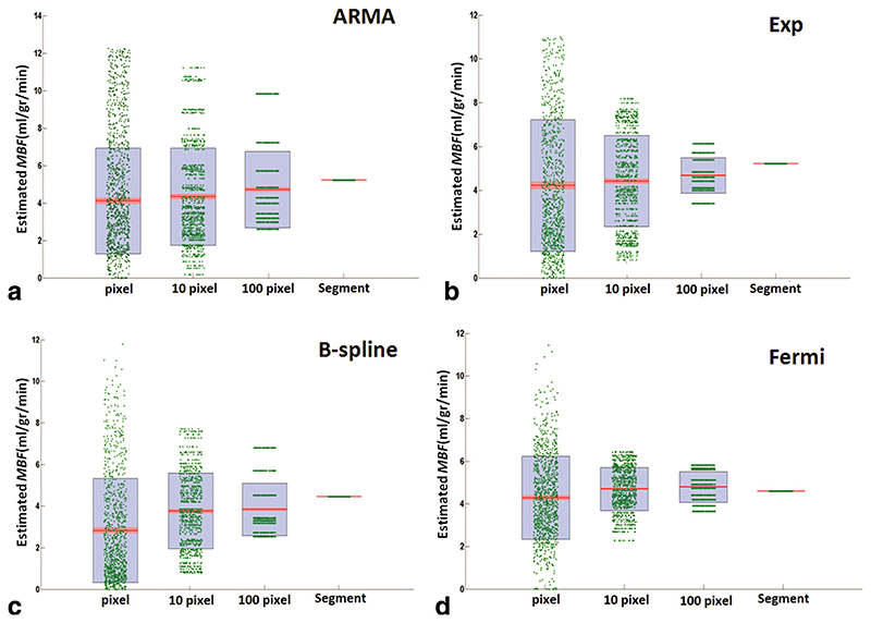
Using first-pass images acquired on the hardware perfusion phantom, perfusion estimates were computed for different perfusion rates on voxel-wise basis and incrementing levels of spatial averaging, i.e., averaging between a group of 10 voxels, 100 voxels, and 600 voxels (the whole slice). Voxel-wise perfusion estimates and results obtained from segmental analysis for different levels of spatial averaging for all four quantification methods are shown in Fig. 3.
Fig. 3.
Scatter-Box plot of estimated MBF in the perfusion phantom experiment, with MBFGS =5 mL/g/min at high CNR (CNR = 32) comparing voxel-wise with segmental analysis, using (a) ARMA, (b) exponential, (c) B-spline, and (d) Fermi method. Each individual green dot shows the estimated MBF at each ROI for different levels of spatial averaging (1 voxel, 10 voxel, 100 voxel, and whole segment), and they have been spread for visualization reasons and clarity. On each blue box, the central red mark is the median; the edges of the box are the 25th and 75th percentiles. The red area around the median shows the points, which are laid over 95% of the confidence interval (the points with less than 5% difference from the median). [Color figure can be viewed in the online issue, which is available at wileyonlinelibrary.com.]
The average estimated perfusion values obtained from the analysis was compared with the true average perfusion rates. Table 3 represents the perfusion estimates relative error (e prl)—defined as absolute error divided by the true average perfusion value—for voxel-wise analysis and segmental analysis.
Table 3. Perfusion Estimates Relative Error (e prl) for Different Levels of Spatial Averaging at MBFGS = 5 ml/g/min (Comparison between Voxel-Wise and Segmental Analysis on Perfusion Phantom Data).
| Level of spatial averaging | ARMA | Exponential | Fermi | B-spline |
|---|---|---|---|---|
| Voxel-wise (610 ROI) | 15.4% | 15.6% | 18% | 43% |
| Segment (one ROI) | 6% | 6.3% | 13%a | 12% |
Note that this value shows the eprl at MBFGS equal to 5 mL/g/ min (high perfusion rate).We expect that the Fermi model to be as accurate as ARMA and exponential at low perfusion values.
With the ARMA, Fermi, and exponential methods, reducing the ROI size from a segment, in which time curves averaged over 610 voxels, to one voxel did not have a significant effect on the estimation accuracy but altered the variability of error.
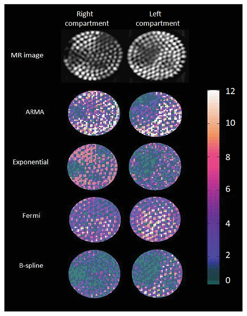
Figure 4 shows MR images of the hardware perfusion phantom and the corresponding perfusion maps using ARMA, exponential, B-spline, and Fermi. The inhomogeneities of flow that are evident in the MR pictures have been captured by voxel-wise perfusion maps.
Fig. 4.
Maps of estimated MBF in perfusion phantom at high input flow rate (5 mL/g/min) and high CNR (CNR = 32) with exponential, ARMA, Fermi, and d B-spline method along with the phantom MR image, which is obtained by calculating maximum intensity projection (MIP)over time of the 10 upslope dynamics. The perfusion inhomogeneity is well depicted with exponential, ARMA, and B-spline model. However, perfusion values are underestimated with B-spline method. Average perfusion value in the reference compartment (left compartment) has been used for calibration. [Color figure can be viewed in the online issue, which is available at wileyonlinelibrary.com.]
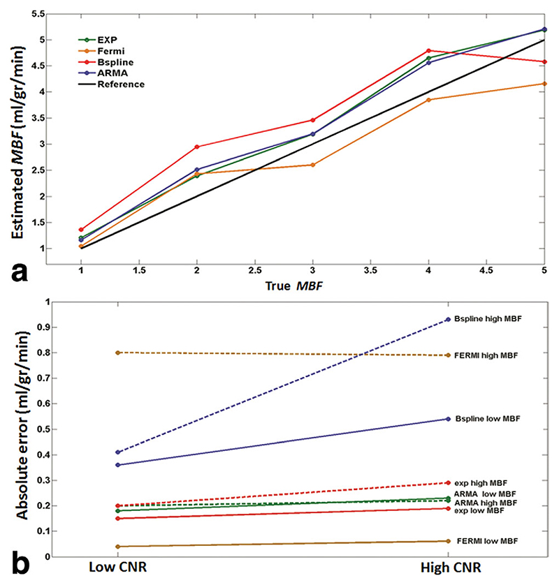
Figure 5a shows a comparison between the mean of estimated perfusion values, averaged over all voxels at each MBF level at high CNR, and true average MBF values from the hardware perfusion phantom.
Fig. 5.
a: Plot of mean of estimated perfusion phantom MBF, averaged over all voxels at each flow level vs. true average flow values at high CNR (CNR = 32) obtained with ARMA, exponential, Fermi, and B-spline method. For flow levels less than 2.5 mL/g/min, the MBF is overestimated with Fermi method and underestimated thereafter. ARMA and exponential method overestimate MBF at all flow levels. At flow levels higher than 4.5 (mL/g/min), MBF is underestimated with B-spline method. True flow values were measured by means of precision flow-meters in the perfusion phantom. b: Perfusion estimates absolute error (e a) in phantom at high CNR (CNR = 32) and low CNR (CNR = 18) obtained with ARMA, exponential, Fermi, and B-spline method using segmental analysis at true average perfusion equal to 1 mL/g/min (dotted lines) and 5 mL/g/min is represented. ARMA, exponential, and Fermi are the least sensitive methods to noise, whereas B-spline results vary significantly with CNR level. Absolute error was relatively constant between different MBF levels for all methods except Fermi (absolute error is high with Fermi model at high flow values). ARMA and exponential methods are more accurate at high perfusion rates compared with Fermi model.
Figure 5b represents the mean of ea averaged over all voxels, at high and low CNR levels and different MBF rates in the perfusion phantom. The difference between ea at high and low CNR for each perfusion level was not significant for ARMA (STD = 0.031 mL/g/min), exponential (STD = 0.028 mL/g/min), and Fermi (STD = 0.014 mL/g/min), whereas it was significant for B-spline (STD = 0.35 mL/g/min). It implies that ARMA, exponential, and Fermi methods are more reliable and robust to noise compared to the B-spline method.
Patient Study
The results obtained from patient studies are shown in Figs. 6–8. The voxel-wise SI curves obtained from the images for all cases had a CNR of 14.6 ± 7.4 before filtering and 27.7 ± 8.4 after temporal and spatial filtering, which are of sufficient quality for accurate analysis (8).
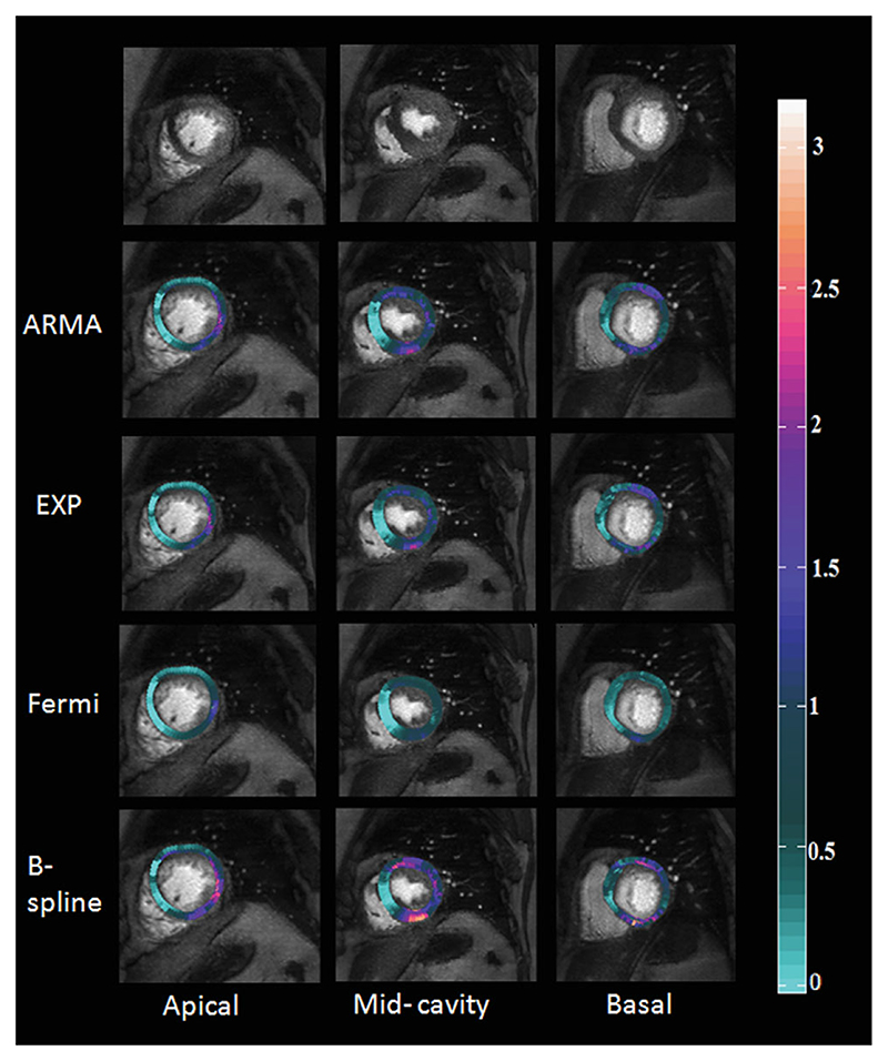
Fig. 6.
Results of voxel-wise perfusion quantification for a 67-year-old female with chronic total occlusion of the LAD collateralized by the LCx. The LCx itself presents a 75% stenosis. The first column from right corresponds to apical layer, the middle-column corresponds to mid-cavity and the last column corresponds to basal layer in myocardium. In the maps, the light green is the worst. The sensitivity of detection of ischemia at the edge of the ischemic area has shown a strict dependency on the used method.
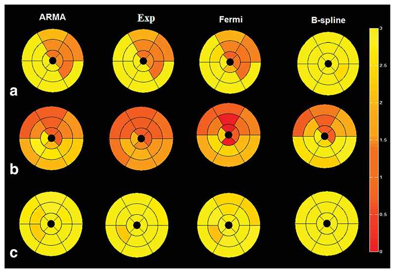
Fig. 8.
Bull’s-eye map of two patients one with (a) LCx disease, (b) LAD disease, and (c) a healthy volunteer comparing the four different methods using American heart association 16 segments representation. MBF values are averaged over all voxels in each segment. It can be seen that there is not a significant variation between different regions of myocardium in the healthy volunteer. The perfusion values are presented in mL/g/min. [Color figure can be viewed in the online issue, which is available at wileyonlinelibrary.com.]
Voxel-wise perfusion maps were generated following MBF analysis using the four models and overlaid over the CMR images from a patient dataset with angina (Fig. 6). Diseased areas are represented as light green and correlate well with the perfusion defects seen in the raw CMR images in the first row. Coronary angiographic findings in this patient demonstrated a chronic total occlusion of the LAD which was collateralized by a 75% stenosed LCx.
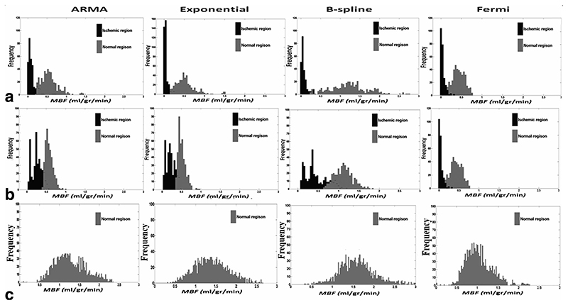
Figure 7a,b represents a histogram comparison of estimated perfusion distribution values in two regions of interest obtained from two patients with proven angiographic coronary artery disease. These graphs demonstrate that voxel-wise analysis allows clear discrimination between normal and ischemic region of myocardium. The ability to correctly distinguish between these regions was different depending on the method used. Figure 7c on the other hand is a histogram example in a healthy volunteer. The volunteer graph (Fig. 7c) yields a single gaussian-shaped graph for the healthy volunteer in comparison to a double gaussian-shaped graph in the patient series.
Fig. 7.
Histogram of estimated MBF comparing distribution of perfusion values obtained by voxel-wise analysis in two regions of interest in (a) 67-year-old male with 2-vessel coronary artery disease and (b) 48-year-old male with one vessel disease affecting the LAD and (c) a healthy volunteer.
It is important to note that the clear delineation of ischemic regions qualitatively illustrated in the perfusion maps achieved statistical significance on quantitative analysis of the differences between the estimated MBF.
Table 4 represents the respective P-value comparison of mean estimated MBF between normal regions and ischemic regions using the four methods. All P values were <0.05 suggesting the presence of significant difference between normal and ischemic regions in abnormal myocardium. The largest discrimination was provided by both ARMA (P < 0.001) and the exponential method (P < 0.005). In contrast, the P-values in healthy volunteers represented in Table 5 are all greater than 0.05 indicating the absence of significant difference between compared regions of interests.
Table 4. The Respective P-Value Comparison of Mean Estimated MBF between Normal Regions and Ischemic Regions Using the Four Methods.
| ARMA | EXP | BSPLINE | FERMI | |
|---|---|---|---|---|
| Patient 1 | 0.000118423 | 6.64E-05 | 0.000112 | 0.025928 |
| Patient 2 | 0.000500101 | 0.001971 | 0.011765 | 0.008551 |
| Patient 3 | 0.00103014 | 0.005226 | 0.012634 | 0.02299 |
| Patient 4 | 0.004675219 | 0.003722 | 0.001875 | 0.001999 |
Table 5. The Respective P-value Comparison of Mean Estimated MBF within Different Regions of Myocardium in Healthy Volunteers Using Different Methods.
| ARMA | EXP | BSPLINE | FERMI | |
|---|---|---|---|---|
| Volunteer 1 | 0.703168828 | 0.819582 | 0.5072 | 0.654329 |
| Volunteer 2 | 0.782779685 | 0.897111 | 0.915155 | 0.89487 |
P value for each volunteer is averaged over three p values which compare LCX segments with RCA segments and LAD segments.
To facilitate clinical utility of these data, the 16 segment American Heart Association model was used to represent the quantified perfusion values. Figure 8 represents the bull’s-eye map of two coronary artery disease patients—(a) with LCx disease and (b) with LAD disease—and a healthy volunteer (c). MBF values are averaged over all voxels in each segment.
Discussion
We believe that this is the first study to demonstrate the feasibility of voxel-wise analysis in detecting underlying ischemia and compare the differences in perfusion estimates, sensitivity to noise, and different levels of spatial averaging between four different deconvolution methods.
First, methods were evaluated with simulated synthetic data. They were then validated with the perfusion phantom, which serves an ideal bridge between synthetic data and patient data. Finally, the validated methods were applied to patient data to show the feasibility of voxel-wise perfusion maps.
The major strength of this study is that we were able to use a phantom as a reference for the different models, flows and noise levels. This is more realistic than synthetic data and thus allows a comparison of the estimated MBF with the true MBF, which is not possible in patients. Here, using the results obtained from phantom experiment, the performance of each method on patients and estimate the accuracy of each method can be predicted.
Based on the more horizontal slope and the low STD displayed in Table 2 and 3, Figs. 2 and 5b, Fermi, ARMA, and exponential model are the least sensitive methods to noise. This characteristic enables a more robust analysis of MBF. However among those three methods, a higher variability of error is observed in ARMA and exponential model compared to Fermi (Fig. 3). This makes Fermi the more favorable method in terms of noise sensitivity for voxel-wise analysis.
ARMA and the exponential method provide the most accurate estimates of MBF among the four methods (e prl < 6.5%) at all MBF levels on an experimental analysis. This is most pronounced at high perfusion rates (Table 2 and Figs. 2 and 5a).
In general, ARMA and the exponential method are more accurate at all flow rates (Figs. 4 and 5), On the other hand, Fermi model is the most robust method to noise with highest precision for voxel-wise analysis. Inevitably, the choice of quantification method for data analysis boils down to a trade off between accuracy and precision of the estimation.
Perfusion maps and histogram graphs indicate that the difference between accuracy of perfusion estimates depend on the selected method. We conjecture that because C aif(t) and C myo(t) curves appear to be approximately biexponential, the exponential bases deconvolution and ARMA method, which can be considered as a generalization of the exponential method (25), provide more accurate and natural tissue kernel and therefore better MBF estimation.
Because voxel-wise analysis offers additional information on the heterogeneity of myocardial perfusion, these results provide a strong case for a voxel-wise approach in clinical applications of DCE-CMR.
Limitations
It is important to note that whilst PET is regarded as the gold standard for the quantification of absolute MBF, we were unable to obtain PET information for this study and compare our results with PET results. The aim of this study was to demonstrate feasibility of a voxel-wise analysis in patients. However, the sample size used here was small, and a larger study examining the correlation between voxel-wise analysis and angiographic findings is currently underway. In addition, a cut-off value for MBF between ischemic and normal regions needs to be addressed by further studies validating the results against appropriate functional tests alongside obtaining histological evidence from animal work.
Further studies are required to investigate the correlation between perfusion estimates in the phantom and patient datasets. In addition, further optimization of the deconvolution methods, including finding the optimal order of considered methods such as ARMA, should be performed.
In this study, we have only used model independent analysis to quantify MBF. A direct comparison of modelindependent and model-dependent analysis will need to be addressed in further studies to define the most appropriate quantitative methods for voxel-wise analysis.
Finally as only one filtering method has been used in the study to remove the noise from signal intensity curves, a further study is needed to analyze the interaction between signal intensities sampling resolutions, temporal, and spatial filtering methods and MBF results obtained from deconvolution analysis.
Conclusions
This study demonstrates the feasibility of voxel-wise quantification of myocardial perfusion on high-resolution MR perfusion data sets. Moreover, it compares different algorithms to determine the most accurate and precise method for voxel-wise MBF quantification. Simulations and maps in patients and hardware phantom showed that voxel-wise quantification of myocardium perfusion is feasible and can be used to detect abnormal regions. The exponential and ARMA methods were more accurate than other methods, whereas Fermi was the most precise and robust method to noise in the voxel-wise analysis of myocardial perfusion.
Acknowledgments
The first two authors named on the title page of this article have contributed equally to the manuscript. They jointly conducted all experiments and data analysis. The authors dedicated to the memory of Dr Philip Batchelor (1967-2011).
References
- 1.Nagel E, Klein C, Paetsch I, Hettwer S, Schnackenburg B, Wegscheider K, Fleck E. Magnetic resonance perfusion measurements for the noninvasive detection of coronary artery disease. Circulation. 2003;108:432–437. doi: 10.1161/01.CIR.0000080915.35024.A9. [DOI] [PubMed] [Google Scholar]
- 2.Al-Saadi N, Nagel E, Gross M, Bornstedt A, Schnackenburg B, Klein C, Klimek W, Oswald H, Fleck E. Noninvasive detection of myocardial ischemia from perfusion reserve based on cardiovascular magnetic resonance. Circulation. 2000;101:1379–1383. doi: 10.1161/01.cir.101.12.1379. [DOI] [PubMed] [Google Scholar]
- 3.Kaufmann PA, Camici PG. Myocardial blood flow measurement by PET: technical aspects and clinical applications. J Nucl Med. 2005;46:75–88. [PubMed] [Google Scholar]
- 4.Pack NA, DiBella EV, Rust TC, Kadrmas DJ, McGann CJ, Butterfield R, Christian PE, Hoffman JM. Estimating myocardial perfusion from dynamic contrast-enhanced CMR with a model-independent deconvolution method. J Cardiovasc Magn Reson. 2008;10:52. doi: 10.1186/1532-429X-10-52. [DOI] [PMC free article] [PubMed] [Google Scholar]
- 5.Pack NA, DiBella EV. Comparison of myocardial perfusion estimates from dynamic contrast-enhanced magnetic resonance imaging with four quantitative analysis methods. Magn Reson Med. 2010;64:125–137. doi: 10.1002/mrm.22282. [DOI] [PMC free article] [PubMed] [Google Scholar]
- 6.Jerosch-Herold M, Wilke N, Stillman AE. Magnetic resonance quantification of the myocardial perfusion reserve with a Fermi function model for constrained deconvolution. Med Phys. 1998;25:73–84. doi: 10.1118/1.598163. [DOI] [PubMed] [Google Scholar]
- 7.Jerosch-Herold M, Swingen C, Seethamraju RT. Myocardial blood flow quantification with MRI by model-independent deconvolution. Med Phys. 2002;29:886–897. doi: 10.1118/1.1473135. [DOI] [PubMed] [Google Scholar]
- 8.Jerosch-Herold M, Seethamraju RT, Swingen CM, Wilke NM, Stillman AE. Analysis of myocardial perfusion MRI. J Magn Reson Imaging. 2004;19:758–770. doi: 10.1002/jmri.20065. [DOI] [PubMed] [Google Scholar]
- 9.Ichihara T, Ishida M, Kitagawa K, Ichikawa Y, Natsume T, Yamaki N, Maeda H, Takeda K, Sakuma H. Quantitative analysis of first-pass contrast-enhanced myocardial perfusion MRI using a Patlak plot method and blood saturation correction. Magn Reson Med. 2009;62:373–383. doi: 10.1002/mrm.22018. [DOI] [PubMed] [Google Scholar]
- 10.Neyran B, Janier MF, Casali C, Revel D, Canet Soulas EP. Mapping myocardial perfusion with an intravascular MR contrast agent: robustness of deconvolution methods at various blood flows. Magn Reson Med. 2002;48:166–179. doi: 10.1002/mrm.10201. [DOI] [PubMed] [Google Scholar]
- 11.Keeling SL, Kogler T, Stollberger R. Deconvolution for DCE-MRI using an exponential approximation basis. Med Image Anal. 2009;13:80–90. doi: 10.1016/j.media.2008.06.011. [DOI] [PubMed] [Google Scholar]
- 12.Larsson HB, Fritz-Hansen T, Rostrup E, Sondergaard L, Ring P, Henriksen O. Myocardial perfusion modeling using MRI. Magn Reson Med. 1996;35:716–726. doi: 10.1002/mrm.1910350513. [DOI] [PubMed] [Google Scholar]
- 13.Jerosch-Herold M. Quantification of myocardial perfusion by cardiovascular magnetic resonance. J Cardiovasc Magn Reson. 2010;12:57. doi: 10.1186/1532-429X-12-57. [DOI] [PMC free article] [PubMed] [Google Scholar]
- 14.Chen H, Li F, Zhao X, Yuan C, Rutt B, Kerwin WS. Extended graphical model for analysis of dynamic contrast-enhanced MRI. Magn Reson Med: Off J Soc Magn Reson Med/ Soc Magn Reson Med. 2011;66:868–878. doi: 10.1002/mrm.22819. [DOI] [PubMed] [Google Scholar]
- 15.Hsu LY, Rhoads KL, Holly JE, Kellman P, Aletras AH, Arai AE. Quantitative myocardial perfusion analysis with a dual-bolus contrast-enhanced first-pass MRI technique in humans. J Magn Reson Imaging. 2006;23:315–322. doi: 10.1002/jmri.20502. [DOI] [PubMed] [Google Scholar]
- 16.Christian TF, Rettmann DW, Aletras AH, Liao SL, Taylor JL, Balaban RS, Arai AE. Absolute myocardial perfusion in canines measured by using dual-bolus first-pass MR imaging. Radiology. 2004;232:677–684. doi: 10.1148/radiol.2323030573. [DOI] [PubMed] [Google Scholar]
- 17.Lee DC, Johnson NP. Quantification of absolute myocardial blood flow by magnetic resonance perfusion imaging. JACC Cardiovasc Imaging. 2009;2:761–770. doi: 10.1016/j.jcmg.2009.04.003. [DOI] [PubMed] [Google Scholar]
- 18.Zierler K. Indicator dilution methods for measuring blood flow, volume, and other properties of biological systems: a brief history and memoir. Ann Biomed Eng. 2000;28:836–848. doi: 10.1114/1.1308496. [DOI] [PubMed] [Google Scholar]
- 19.Sourbron S, Dujardin M, Makkat S, Luypaert R. Pixel-by-pixel deconvolution of bolus-tracking data: optimization and implementation. Phys Med Biol. 2007;52:429–447. doi: 10.1088/0031-9155/52/2/009. [DOI] [PubMed] [Google Scholar]
- 20.Makkat S, Luypaert R, Sourbron S, Stadnik T, De Mey J. Quantification of perfusion and permeability in breast tumors with a deconvolution-based analysis of second-bolus T1-DCE data. J Magn Reson Imaging. 2007;25:1159–1167. doi: 10.1002/jmri.20937. [DOI] [PubMed] [Google Scholar]
- 21.Iaizzo PA. Handbook of cardiac anatomy, physiology, and devices. xiii. Humana Press; Totowa, N.J: 2005. p. 469. [Google Scholar]
- 22.Gill PE, Murray W, Wright MH. Practical optimization. xvi. Academic Press; London: 1981. p. 401. [Google Scholar]
- 23.Engl HW, Hanke M, Neubauer A. Regularization of inverse problems. viii. Kluwer Academic Publishers; Dordrecht: 1996. p. 321. [Google Scholar]
- 24.Wilke N, Jerosch-Herold M, Wang Y, Huang Y, Christensen BV, Stillman AE, Ugurbil K, McDonald K, Wilson RF. Myocardial perfusion reserve: assessment with multisection, quantitative, first-pass MR imaging. Radiology. 1997;204:373–384. doi: 10.1148/radiology.204.2.9240523. [DOI] [PubMed] [Google Scholar]
- 25.Batchelor P, Chiribiri A, Nooralipour NZ, Cvetkovic Z. Arma regularization of cardiac perfusion modeling; International Conference on Acoustics, Speech and Signal Processing, ICASSP 2010; 2010. pp. 642–645. [Google Scholar]
- 26.Schumaker LL. Spline functions : basic theory. Cambridge University Press; New York: 2007. p. 582. [Google Scholar]
- 27.Hansen PC. Analysis of discrete ill-posed problems by means of the L-curve. Siam Rev. 1992;34:561–580. [Google Scholar]
- 28.Kashyap RL. Optimal choice of ar and ma parts in autoregressive moving average models. IEEE Trans Pattern Anal Mach Intell. 1982;4:99–104. doi: 10.1109/tpami.1982.4767213. [DOI] [PubMed] [Google Scholar]
- 29.Degooijer JG, Abraham B, Gould A, Robinson L. Methods for determining the order of an autoregressive-moving average process—a survey. Int Stat Rev. 1985;53:301–329. [Google Scholar]
- 30.Lindsey JK, Byrom WD, Wang J, Jarvis P, Jones B. Generalized nonlinear models for pharmacokinetic data. Biometrics. 2000;56:81–88. doi: 10.1111/j.0006-341x.2000.00081.x. [DOI] [PubMed] [Google Scholar]
- 31.Gudbjartsson H, Patz S. The Rician distribution of noisy MRI data. Magn Reson Med. 1995;34:910–914. doi: 10.1002/mrm.1910340618. [DOI] [PMC free article] [PubMed] [Google Scholar]
- 32.Rajan J, Poot D, Juntu J, Sijbers J. Noise measurement from magnitude MRI using local estimates of variance and skewness. Phys Med Biol. 2010;55:N441–N449. doi: 10.1088/0031-9155/55/16/N02. [DOI] [PubMed] [Google Scholar]
- 33.Ishida M, Schuster A, Morton G, Chiribiri A, Hussain S, Paul M, Merkle N, Steen H, Lossnitzer D, Schnackenburg B, Alfakih K, et al. Development of a universal dual-bolus injection scheme for the quantitative assessment of myocardial perfusion cardiovascular magnetic resonance. J Cardiovasc Magn Reson. 2011;13:28. doi: 10.1186/1532-429X-13-28. [DOI] [PMC free article] [PubMed] [Google Scholar]
- 34.Chiribiri A, Schuster A, Ishida M, Hautvast G, Zarinabadnooralipour N, Paul M, Hussain S, Batchelor P, Breeuwer M, Schaeffter T, Nagel E. Dynamic simulation of first pass myocardial perfusion MR with a novel perfusion phantom. J Cardiovasc Magn Reson. 2011;13:46. [Google Scholar]
- 35.Plein S, Ryf S, Schwitter J, Radjenovic A, Boesiger P, Kozerke S. Dynamic contrast-enhanced myocardial perfusion MRI accelerated with k-t sense. Magn Reson Med. 2007;58:777–785. doi: 10.1002/mrm.21381. [DOI] [PubMed] [Google Scholar]
- 36.Plein S, Schwitter J, Suerder D, Greenwood JP, Boesiger P, Kozerke S. k-Space and time sensitivity encoding-accelerated myocardial perfusion MR imaging at 3.0 T: comparison with 1.5 T. Radiology. 2008;249:493–500. doi: 10.1148/radiol.2492080017. [DOI] [PMC free article] [PubMed] [Google Scholar]
- 37.Gebker R, Jahnke C, Paetsch I, Schnackenburg B, Kozerke S, Bornstedt A, Fleck E, Nagel E. MR myocardial perfusion imaging with k-space and time broad-use linear acquisition speed-up technique: feasibility study. Radiology. 2007;245:863–871. doi: 10.1148/radiol.2453061701. [DOI] [PubMed] [Google Scholar]
- 38.Breeuwer M, Quist M, Spreeuwers L. Automatic quantitative analysis of cardiac mr perfusion images; Proceedings of SPIE Medical Imaging; San Diego, CA, USA. 2001. pp. 733–742. [Google Scholar]
- 39.Spreeuwers L, Breeuwer M. Automatic detection of myocardial boundaries in MR cardio perfusion images; Proceedings of Medical Image Computing and Computer-Assisted Intervention; Utrecht, Netherlands. 2001. pp. 1228–1231. [Google Scholar]
- 40.Di Bella EV, Wu YJ, Alexander AL, Parker DL, Green D, McGann CJ. Comparison of temporal filtering methods for dynamic contrast MRI myocardial perfusion studies. Magn Reson Med: Off J Soc Magn Reson Med/Soc Magn Reson Med. 2003;49:895–902. doi: 10.1002/mrm.10439. [DOI] [PubMed] [Google Scholar]


