An open approach to systematically prioritize causal variants and genes at all published human GWAS trait-associated loci

Abstract

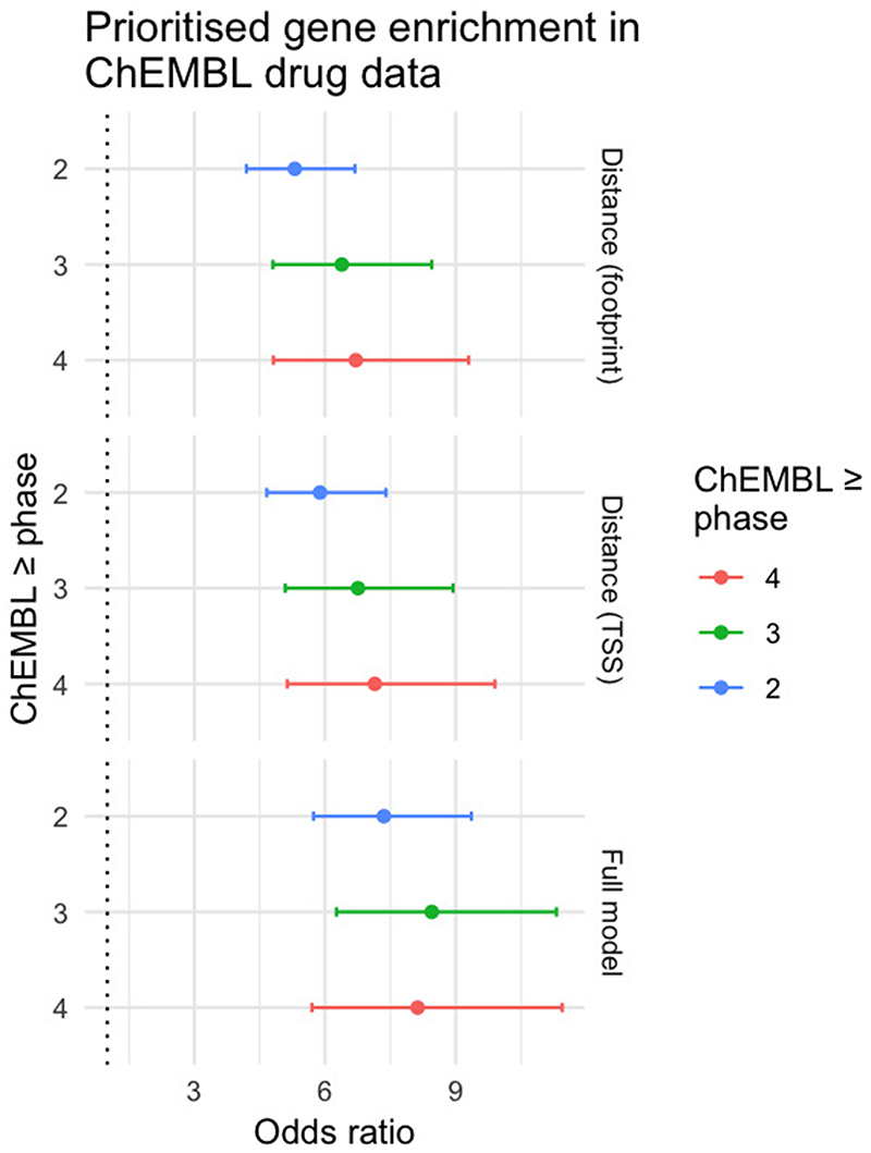
Genome-wide association studies (GWAS) have identified many variants associated with complex traits, but identifying the causal gene(s) is a major challenge. Here we present an open resource that provides systematic fine-mapping and gene prioritization across 133,441 published human GWAS loci. We integrate genetics (GWAS Catalog and UK Biobank) with transcriptomic, proteomic and epigenomic data, including systematic disease-disease and disease-molecular trait colocalization results across 92 cell types and tissues. We identify 729 loci fine-mapped to a single coding causal variant and colocalized with a single gene. We trained a machine learning model using the fine-mapped genetics and functional genomics data using 445 gold-standard curated GWAS loci to distinguish causal genes from neighboring, outperforming a naive distance-based model. Our prioritized genes were enriched for known approved drug targets (OR = 8.1, 95% CI: (5.7, 11.5)). These results are publicly available through a web portal (http://genetics.opentargets.org), enabling users to easily prioritize genes at disease-associated loci and assess their potential as drug targets.

Over 90% of GWAS trait-associated SNPs fall in non-coding regions, indicating that they affect expression of neighboring genes through regulatory mechanisms^1,2, which can act over long distances and affect more than one gene. Hence, identifying the causal gene(s) and cell or tissue site of action is a major challenge requiring detailed low-throughput analysis of individual loci. One default approach has been to assign the top trait-associated SNP to the closest gene at each locus. However relying on physical proximity alone can be misleading since SNPs can influence gene expression over long genomic ranges³, with studies based on eQTL data suggesting that two-thirds of the causal genes at GWAS loci are not the closest^4,5. To add to the challenge, associated SNPs often span large regions due to linkage disequilibrium (LD), and pinning down the functional SNP and the tissue or cell type that mediates its effect can be complicated.

Connecting causal variants with their likely causal gene is a laborious process that requires the integration of GWAS data with multi-omics datasets across a wide range of cell types and tissues such as RNA expression, protein abundance, chromatin accessibility and chromatin interaction datasets. Subsequent functional assessment (such as reporter assays and CRISPR/Cas9 genome editing) can then be used to confirm the relationship between a putative causal variant and the gene it regulates. Using these integrative approaches, systematic international efforts have been undertaken to translate GWAS trait-associated signals into target genes focused on one or a small subset of phenotypes^6–9. However, there are currently no resources that systematically prioritize all genes beyond specific therapy areas⁹. Therefore, there is a need for a comprehensive, unbiased, scalable and reproducible approach that leverages all the publicly available data and knowledge to assign genes systematically to published loci across the entire range of phenotypes and diseases.

Drug development is hindered by a high attrition rate, with over 90% of the drugs that enter clinical trials failing, primarily due to lack of efficacy found in later, more costly stages of development¹⁰. Retrospective analyses have estimated that drugs are twice as likely to be approved for clinical use if their target is supported by underlying GWAS evidence¹¹. Hence, there is a critical need to build strategies that incorporate novel genetic discoveries and mechanistic evidence from GWAS and post-GWAS studies to suggest novel therapeutic targets for which to develop medicines, and ultimately increase the success rate of drug development.

Here we describe a universal solution to these challenges: a systematic and comprehensive analysis pipeline for integrating GWAS results with functional genomics data to prioritize the causal gene(s) at each published GWAS trait-associated locus. The pipeline performs fine-mapping and systematic disease-disease and disease-molecular trait colocalization analysis. We integrate information from GWAS, expression and protein quantitative trait loci (eQTL and pQTL) and epigenomics data (e.g. promoter capture Hi-C, DNase hypersensitivity sites). For gene prioritization, we developed a machine learning model trained on a set of 445 curated gold-standard GWAS loci for which we have moderate or strong confidence in the functionally implicated gene. The model integrates the fine-mapping with the functional genomics data, gene distance, and in silico functional predictions to link each locus to its target gene(s). This output of this pipeline feeds into Open Targets Genetics (https://genetics.opentargets.org), a user-friendly, freely available, integrative web portal enabling users to easily prioritize likely causal variants and target genes at all loci and assess their potential as pharmaceutical targets through linking out to Open Targets Platform^12,13,14, and will be regularly updated as new data become available.

Results

Pipeline overview

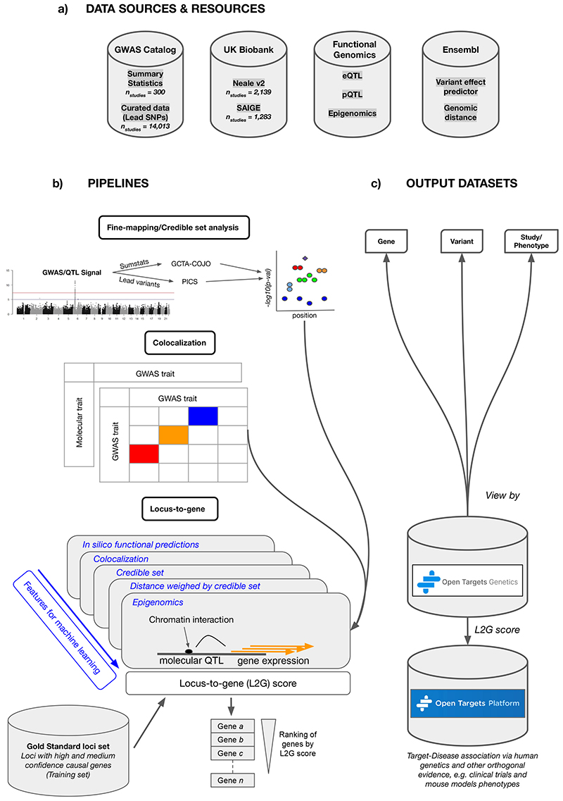
We harmonized and processed GWAS data from the GWAS Catalog and from UK Biobank and conducted systematic fine mapping to generate sets of credibly causal variants across all 133,441 study-lead variant associated loci. We also conducted cross-trait colocalization analyses for 3,621 GWAS datasets with summary statistics available, which enabled us to identify traits and diseases that share common genetic etiology and mechanisms. To investigate whether changes in gene expression and protein abundance influence trait variation and disease susceptibility, we integrated 92 tissue- and cell type-specific molecular QTL datasets including GTEx¹⁵, eQTLGen¹⁶, the eQTL Catalogue¹⁷ and pQTLs¹⁸ and conducted systematic disease-molecular trait colocalization tests. Finally, we used a machine learning framework based on fine mapping, colocalization, functional genomics data and distance to prioritize likely causal genes at all trait-associated loci (Fig. 1).

Figure 1. Open Targets Genetics pipeline schematic.

a, Data sources include all available GWAS, as well as variant effect predictions and functional genomic data. b, A number of pipelines are run to perform statistical fine-mapping of GWAS, colocalization with gene expression quantitative trait studies (QTLs) and also between distinct GWAS traits, and integrative “locus-to-gene” prioritization from both genetic and functional genomic input features. c, Outputs of the pipelines are available in a web portal, via programmatic API, and as bulk downloads.

Fine mapping of all published genome-wide association studies

To establish a comprehensive resource linking variants and traits or diseases, we integrate GWAS studies both with and without full summary statistics. Full summary statistics were obtained from three sources: the NHGRI-EBI GWAS Catalog summary statistics database (number of studies (n _study) = 300)¹⁹; binary phenotypes from UK Biobank as published by Zhou et al. (n _study = 1,283)²⁰ and all other UK Biobank phenotypes from the Neale lab (n _study = 2,139; downloaded 21 January 2019)²¹. Studies with full summary statistics were restricted to those of predominantly European ancestries due to the lack of suitable reference genotypes required for conditional analysis from other populations. Studies without full summary statistics included all others in the NHGRI-EBI GWAS Catalog (n _study = 14,013)¹⁹. To prioritize candidate causal variants at each GWAS association, we performed fine mapping of 10,494 GWAS Catalog and UK Biobank studies. Two fine-mapping methods were used to maximize coverage of GWAS studies, one using full summary statistics and a second using LD information only (see Methods). For studies with full summary statistics, we first identified independent signals using GCTA-COJO²² and then conducted per-signal conditional analysis adjusting for other independent signals in a region ±2 Mb from the sentinel variant. We then used the Approximate Bayes Factor approach²³ to fine-map each conditionally independent signal. For studies without summary statistics, we used the PICS method²⁴ with an LD reference from the most closely matched 1000 Genomes superpopulation to estimate the probability that each variant is causal. Both methods output a posterior probability (PP) for each variant to be causal for the given association.

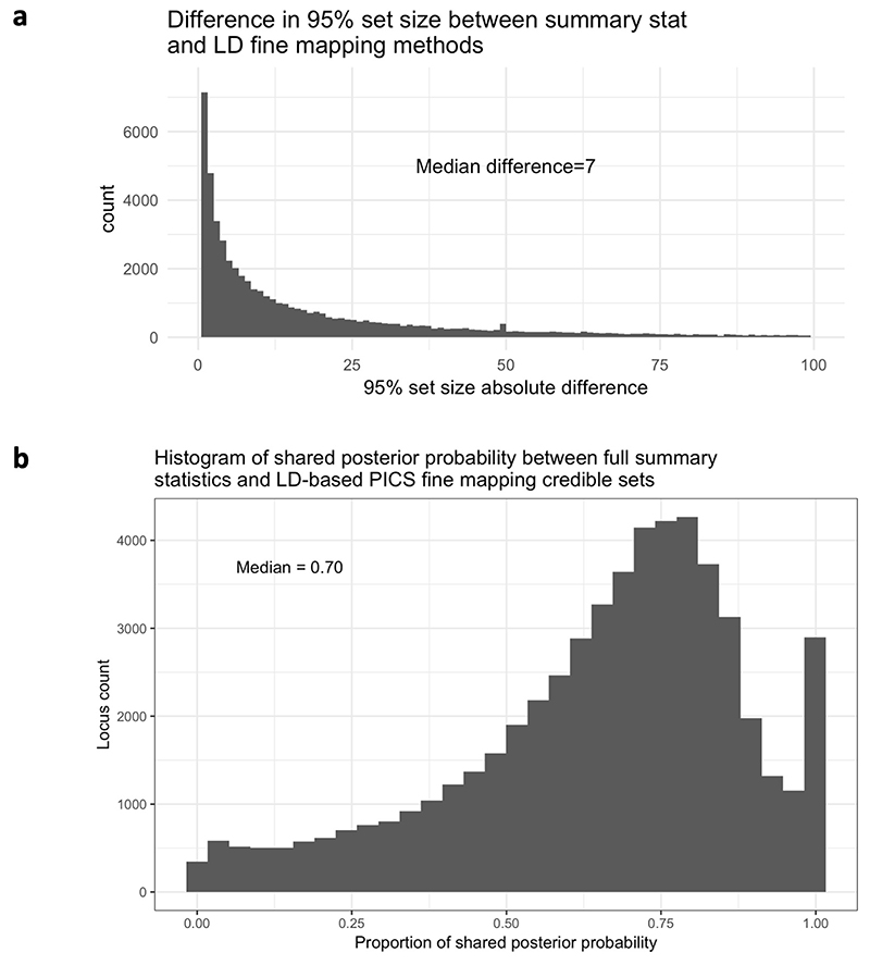
We detected a total of 133,441 sentinel variants, with 53% of these being shared by more than one study (70,860 distinct sentinel variants). To assess the concordance of the two methods, we compared the 95% credible sets after applying both methods to all loci from studies with summary statistics available. We found a median absolute difference in credible set size of 7 variants (Fig. 1a and Extended Data Fig. 1a), whereas the median credible set contained 17 variants. On average across loci, 70% of the credible set posterior probability colocated to the same variants between the two methods (Extended Data Fig. 1b). These results suggest that on average the methods produced comparable results. For subsequent analyses, we therefore used the full summary statistics method where these data were available, and for studies without summary statistics we used the PICS method.

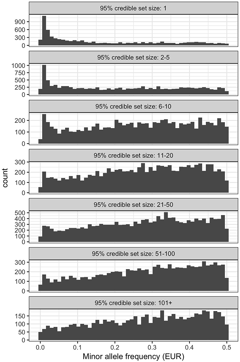
Out of 133,441 association signals, 12,500 (9%) could be resolved to a single variant having PP > 0.95 and a further 21,279 (16%) to between 2 and 5 likely causal variants. Association signals with smaller credible sets were enriched for having rarer variants as the lead variant (Extended Data Fig. 2). Single-variant credible sets were 8.5 times more likely to have a moderate or high impact on protein-coding transcripts as predicted by the Ensembl variant effect predictor (VEP)²⁵ compared to variants in credible sets with 2 or more variants (OR = 8.51, P < 2.2 × 10^-16, Fisher’s exact test). Outside coding regions, single-variant credible set variants were preferentially located in Ensembl Regulatory Build regulatory elements, including promoters (OR = 1.70, P < 2.2 × 10^-16), enhancers (OR = 1.09, P = 4.08 × 10^-4), transcription factor binding motifs (OR = 1.85, P = 1.22 × 10^-15) or other open chromatin regions (OR = 1.19, P = 4.8 × 10^-5).

In order to identify GWAS signals with high-confidence evidence linking the trait to variant and variant to gene, we took single-variant resolution loci and filtered these to retain variants with moderate or high-impact coding consequences in VEP. We identified 2,284 single coding variants linking 378 genes to 303 traits (Supplementary Table 1). Among these were several known disease-causal gene associations and targets of approved therapies (Supplementary Table 2) as well as novel disease-causal gene associations that had no prior evidence in the Open Targets Platform. One example is rs35383942, associated with breast cancer^20,26, which is a predicted deleterious missense variant (Arg28Gln, CADD = 24.3) in PHLDA3 (Pleckstrin Homology Like Domain Family A Member 3). PHLDA3 is the direct target of TP53 and acts as a tumor suppressor gene through inhibition of AKT1, an oncogene that plays a pivotal role in cell proliferation and survival²⁷.

Colocalization of GWAS and molecular traits

Since most associated variants are non-coding, it is expected that they influence disease risk through altering gene expression or splicing. One way to identify the target gene is to demonstrate that the statistical association of a GWAS locus and a gene expression QTL are colocalized—that is, that the pattern of SNP associations is consistent with them sharing the same causal variant. We conducted systematic colocalization analysis²⁸ of GWAS loci with molecular trait QTLs from 92 tissues or cell types. The QTL datasets (Supplementary Table 3) include pQTLs for 2,994 plasma proteins assessed in 3,301 individuals of European descent¹⁸, eQTLs from 48 GTEx tissues (v7.0), blood eQTLGen¹⁶, and 14 eQTL studies from the newly established eQTL Catalogue, a resource of uniformly processed gene expression and splicing QTLs recomputed from previously published datasets¹⁷. The results of the colocalization test are summarized by the probability, referred to as “H4”, that a causal variant is shared.

GWAS-molecular QTL loci were tested if there was at least 1 variant overlapping in their 95% credible sets, suggesting prior evidence for colocalization (see Methods). Of the 70,364 trait-associated loci from studies with summary statistics available, 49.4% had no colocalizing gene at an H4 threshold > 0.8, 25.5% had exactly 1 colocalizing gene, and 25.2% had >1 colocalizing gene. For loci with evidence of colocalization between GWAS and molecular QTL traits, 29% were specific to a single tissue or cell type, whereas 71% were observed across multiple tissues. We also examined non-coding QTLs that were fine-mapped to a single-variant resolution and that colocalized with binary trait GWAS signals (H4 > 0.95). Results from this analysis are summarized in Supplementary Table 4.

We also performed cross-trait colocalization across 3,621 GWAS datasets to identify traits that are likely to be underpinned by the same molecular mechanism. A summary of the binary trait GWAS loci with the highest colocalization score (H4 > 0.95) is displayed in Supplementary Table 5. One example is a locus on chromosome 6 that colocalizes with asthma (6_90220794_T_C) and Crohn’s disease (6_90263440_C_A), suggesting that the two diseases may share common genetic etiology at this locus.

To demonstrate the value of colocalization evidence, we examined coding variants that were fine-mapped to single-variant resolution and that colocalized with a molecular QTL for the same gene (729 variants, Supplementary Table 6). Such cis-variants make good genetic instruments for testing the causal effect of the molecular phenotype on disease²⁹, and the ratio of coefficients for the cis-variants is an estimate of the effect size of the molecular phenotype on disease. Using this approach, we identified several known gene-trait associations. For example, missense variant rs34324219 is causal of changes in TCN1 RNA and protein expression in whole blood^16,18 and also colocalizes (H4 > 0.99) with pernicious anemia, a disorder in which too few red blood cells are produced due to vitamin B12 deficiency. TCN1 encodes the protein haptocorrin (also known as Transcobalamin-1), which binds vitamin B12 and is involved in its uptake³⁰. Also, splice region variant rs1893592 causes increased expression of UBASH3A in most GTEx tissues, including thyroid. This signal colocalizes (H4 > 0.87) with self-reported treatment using the thyroid hormone sodium levothyroxine. Hypothyroidism is a common comorbidity with type 1 diabetes, for which there is strong evidence that UBASH3A is causal for disease risk³¹. Finally, the synonymous variant rs2228079 is the only credibly causal variant for an eQTL associated with altered ADORA1 expression in whole blood (eQTLGen) and colocalizes with asthma in UK Biobank (H4 > 0.99). ADORA1 encodes a type of adenosine receptor, a class of proteins targeted by an approved drug (Theophylline) for the treatment of asthma.

Colocalization also provided strong genetic evidence for some less well known gene-disease associations (Supplementary Table 7). One example is splice region variant rs11589479, which causes increase in ADAM15 expression in several monocytes states and also colocalizes (H4 = 0.99) with Crohn’s disease³². ADAM15, a disintegrin and metalloproteinase, is strongly upregulated in colon tissues from inflammatory bowel disease patients compared to healthy controls and plays a role in leukocyte trans-migration across epithelial and endothelial barriers as well as the differentiation of regenerative colonic mucosa³³.

A machine learning model prioritizes genes at gold-standard loci

We next developed a “locus to gene” model (L2G) to prioritize causal protein-coding genes at GWAS loci by integrating our catalog of fine-mapped associations with relevant functional genomics features. We first manually curated a set of 445 gold-standard positive (GSP) genes at GWAS loci for which we are confident of the causal gene assignment (Supplementary Table 8, see Methods). The selected genes are based on: (i) expert domain knowledge of strong orthogonal evidence or biological plausibility; (ii) known drug target-disease pairs; (iii) experimental alteration from literature reports (e.g. nucleotide editing); (iv) observational functional data (e.g. colocalizing molecular QTLs, colocalizing epigenetics marks, reporter assays) (Supplementary Table 9). Next, we defined locus-level predictive features from four evidence categories: in silico pathogenicity prediction from VEP and PolyPhen, colocalization of molecular QTLs, gene distance to credible set variants weighted by their fine-mapping probabilities, and chromatin interaction (Extended Data Fig. 3 and Supplementary Tables 10 and 11). The chromatin interaction data comprised promoter-capture Hi-C from 27 cell types³⁴, FANTOM enhancer-TSS pairwise cap analysis of gene expression (CAGE) correlation³⁵, and DNase I hypersensitive site-gene promoter correlation³⁶. Then, using a nested cross-validation strategy, we trained a gradient boosting model to distinguish GSP genes from other genes within 500 kb at the same loci (see Methods).

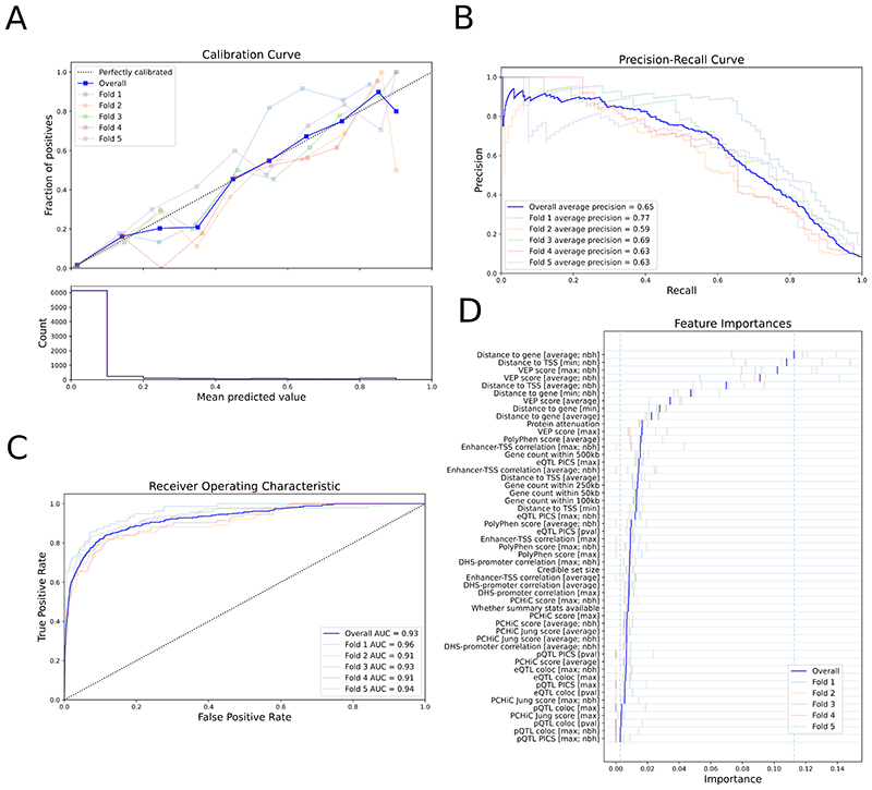
The L2G model produced a well calibrated score, ranging from 0 to 1, which reflects the approximate fraction of GSP genes among all genes above a given threshold (Fig. 2). At a classification threshold of ≥ 0.5, the full model correctly identified 238 out of 445 true positives with 86 false positives (average precision = 0.65; Table 1). We compared the full model against a naive nearest gene classifier (closest gene footprint and closest TSS), which selects the closest gene to each lead variant and thus does not make use of other candidate variants from fine-mapping. The naive nearest gene classifier identified more true positives at the same threshold (268 out of 445) but at the cost of identifying 2.4 times more false positives (207) (average precision = 0.37). Hence, the full L2G model has higher precision with a small reduction in recall.

Figure 2. Performance of the locus-to-gene (L2G) model.

Colors show metrics calculated on each individual fold of the 5-fold cross-validation. The overall metric, combining all folds, is shown in dark blue. a, Calibration curve showing (top) the fraction of all GSP genes found as positives at different L2G score thresholds (mean predicted value) and (bottom) the count of genes in each L2G score bin. b,c, The precision-recall curve (b) and the receiver-operator characteristic curve (c) for identifying GSP genes from among those within 500 kb at each locus. d, The Relative Importance of each predictor in the L2G model. Blue vertical bars show the mean importance for each feature in cross-validation, while paler bars show the importance obtained in each fold. The vertical dashed lines show the minimum and maximum mean feature importances. max denotes that the maximum score for any variant in the 95% credible set was used for each gene; average denotes that a score averaged over the 95% credible set, weighted by posterior probability, was used for each gene; nbh (neighbourhood) denotes that scores were calculated for each gene relative to the best scoring gene at the locus. Insets in a-c indicate the chromosomes for which each fold of the data was evaluated in cross-validation, and the average precision (AP) (b) or AUC (c) for that fold.

Table 1. Classification performance for feature groups.

Performance characteristics of the full model are shown at the top, and analyses for individual groups of features are shown in sections below. Counts are shown for true positives (TP), false positives (FP), true negatives (TN), and false negatives (FN). *Mean distance aggregates across all the variants in the credible set and weighs by their posterior probability.

Features	Average precision	AUC	Precision	Recall	TP	FP	TN	FN	Sensitivity	Specificity	FDR	GSP count	GSN count
Full model	0.65	0.93	0.73	0.53	236	86	6,429	209	0.53	0.99	0.27	445	6,515
Naïve closest gene classification
Closest footprint	0.37	0.79	0.56	0.60	268	207	6,308	177	0.60	0.97	0.44	445	6,515
Closest TSS	0.34	0.76	0.56	0.55	246	195	6,320	199	0.55	0.97	0.44	445	6,515
Leave-one-group-in
Mean distance*	0.62	0.91	0.69	0.49	219	98	6,417	226	0.49	0.98	0.31	445	6,515
Interaction	0.26	0.79	0.55	0.05	23	19	6,496	422	0.05	1.00	0.45	445	6,515
Molecular QTL	0.36	0.85	0.62	0.18	79	49	6,466	366	0.18	0.99	0.38	445	6,515
Pathogenicity prediction	0.48	0.76	0.70	0.43	191	80	6,435	254	0.43	0.99	0.30	445	6,515
Leave-one-group-out
Mean distance*	0.47	0.77	0.69	0.43	191	84	6,431	254	0.43	0.99	0.31	445	6,515
Interaction	0.65	0.93	0.73	0.53	234	85	6,430	211	0.53	0.99	0.27	445	6,515
Molecular QTL	0.65	0.93	0.74	0.54	239	86	6,429	206	0.54	0.99	0.26	445	6,515
Pathogenicity prediction	0.63	0.92	0.71	0.50	222	91	6,424	223	0.50	0.99	0.29	445	6,515

To identify which features are most important in predicting GSP genes, we retrained the model to include features from only one of the four evidence categories at a time (leave-one-group-in analysis). No individual feature set gets a higher ‘Average Prediction’ score as the full model (Table 1). Our ‘mean distance’ feature, which aggregates across all the variants in the credible set and weighs by their posterior probability, was the most predictive (average precision = 0.62), followed by in silico pathogenicity prediction evidence (average precision = 0.48), molecular QTL colocalization (average precision = 0.36) and chromatin interaction (average precision = 0.26) (Table 1, leave-one-group-in section). Note that the ‘mean distance’ feature is distinct from a ‘naive closest gene distance’ feature because of the weighting across a credible set to the most likely SNPs, and thus manages to discard many false positives (FP_{mean distance} = 98 vs. FP_{naive closest footprint gene} = 207 and FP_{naive closest TSS gene} = 195). Within the mean distance features tested, whether the gene was the closest at the locus using a gene footprint distance metric averaged over the credible set and whether the gene was the closest at the locus using the minimum gene-TSS distance over the 95% credible set had the highest relative feature importances (Fig. 2d). Thus, when using distance as a predictor of causal genes, the distance relative to other genes is more important than the absolute distance.

We also assessed the unique contribution of each evidence type by leaving out one group of features at a time. Consistent with the leave-one-group-in analysis, dropping our mean distance features had the largest impact on prediction (average precision change from 0.65 to 0.47), followed by in silico pathogenicity prediction (average precision down to 0.63) (Table 1). Notably, when molecular QTL colocalization evidence was removed from the model, we saw similar classification results, with 3 fewer true positives identified, and no net change in the Gold Standard Negatives (GSN) (Supplementary Table 12a). There are various possible reasons for this: the colocalization score may be redundant with some of our other features, we may lack the relevant tissue- or context-specific QTLs, or we may have obscured the utility of colocalization information by using a cross-tissue colocalization score. The relatively high importance of distance remained when we trained the model on the 352 gold-standard loci lacking a detrimental coding variant (Supplementary Table 13). We also used a measure of continuous reclassification improvement to evaluate prediction changes across all possible classification thresholds. Here, adding molecular QTL colocalization evidence resulted in a net 4.7% GSPs having an increased prediction score and a net 42.2% GSNs having a decreased score (Supplementary Table 12b). This suggests that, while our colocalization features do not provide sufficient evidence to support novel positives, lack of colocalization accurately identifies negative gene assignments. Removing chromatin interaction features resulted in a minor reduction in model performance (net 2 fewer GSPs) (Table 1).

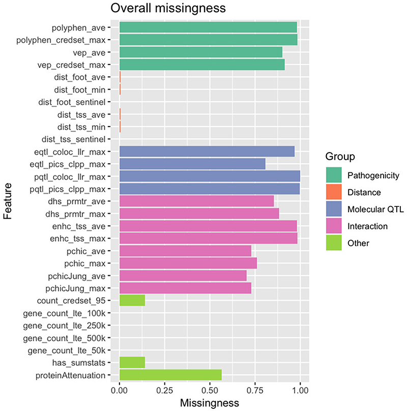
The low predictiveness of features apart from distance relates in part to their lower genome coverage. For distance features, most sentinel variants have at least 1 gene within 500 kb, but for pathogenicity, molecular QTL colocalization and chromatin interaction, coverage of variants was low (Extended Data Fig. 4). Only a small proportion of studies had summary statistics available, limiting our ability to use coloc to perform a colocalization analysis (only 3% of all loci had coloc derived evidence). Our complementary colocalization method, using a reference LD-panel to approximate summary statistics (the PICS method), increased the total number of loci with colocalization evidence to 19%. Evidence from pQTLs was very sparse at <1% coverage, which may account for its very low feature importance (Extended Data Fig. 4).

Gene prioritization across all trait-associated loci

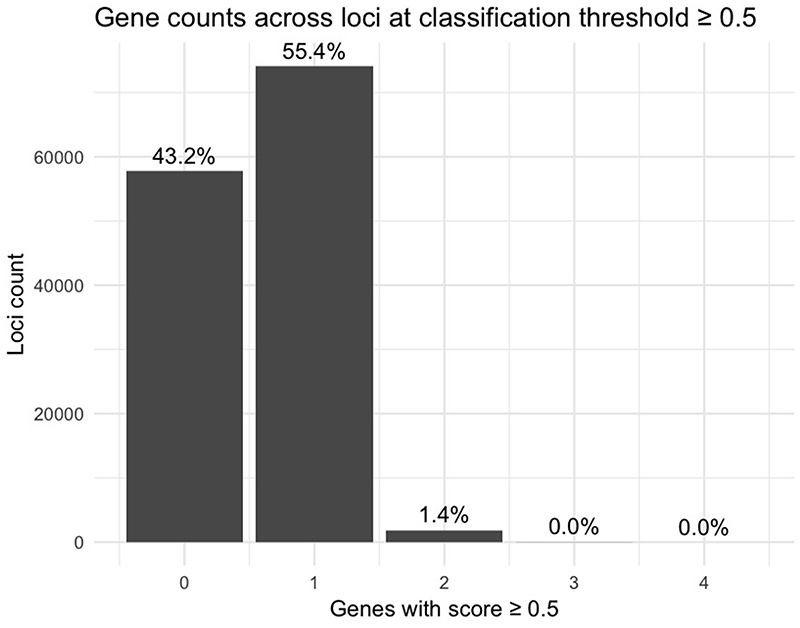
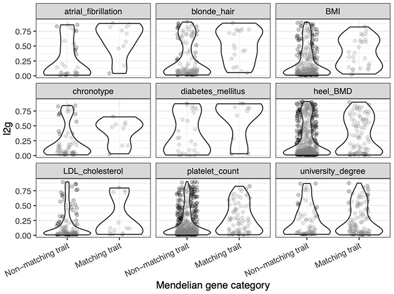
We used the trained L2G model to prioritize causal genes across all 133,441 trait-associated GWAS loci in our repository. At a classification threshold of 0.5, 55.4% (n = 74,096) of all loci had a single gene prioritized whereas only 1.4% (n = 1,907) had 2 or more genes prioritized (Extended Data Fig. 5). 43.2% of loci did not reach the classification threshold. Across all diseases, genes prioritized by the model were 7.8 times more likely (95% CI: (6.5, 9.3)) to be supported by literature evidence identified by text mining (Supplementary Table 14). Genes prioritized by the naive classifier using the closest gene footprint from the sentinel variant were also enriched (5.6 times, 95% CI: (4.7, 6.6)) but not as highly as the full model (P = 0.008 against null-hypothesis logOR_{Full model} = logOR_{Naive model}, Welch t-test). In a selection of nine GWAS traits, Mendelian disease genes with matching phenotypes were enriched for having high L2G scores relative to non-matching Mendelian disease genes (Extended Data Fig. 6), supporting the utility of L2G in prioritizing relevant genes.

In order to benchmark the L2G versus the distance-based classifier, we tested whether prioritized gene-diseases were enriched for known drug target-indication pairs across different clinical phases according to the ChEMBL database. Genes prioritized by the model were enriched with OR 7.4, 8.5 and 8.1 (95% CI: (5.7, 9.4), (6.3, 11.3), (5.7, 11.5)) across clinical trial phases ≥2, ≥3 and 4, respectively (Supplementary Table 15). Using a naive classifier, we saw lower odds ratio point estimates but with overlapping confidence intervals (OR 5.3 (4.2, 6.7), 6.4 (4.8, 8.5) and 6.7 (4.8, 9.3)) (Extended Data Fig. 7). Thus, the prioritization using the L2G model recapitulates the established enrichment of GWAS loci for known drugs¹¹ but also demonstrates that fine-mapping and colocalization combined with the L2G model improves on their approach, and hence is likely to also improve success in identifying novel drug targets.

Discussion

To address the challenges of translating GWAS signals to biological insights, we developed a pipeline to format, harmonize, and aggregate human trait and disease GWAS, molecular QTLs and functional genomics data in a consistent way, providing statistical evidence for target prioritization across the entirety of GWAS traits and diseases. We then trained a machine learning model that integrates fine-mapping and functional genomics data to prioritize likely causal variants and genes at 133,441 trait-lead variant disease associations. The L2G score output by the model represents the likelihood that a gene is causal for that trait, subject to the limitations of our gold-standard positive training data, and thus allows genes at all trait-associated loci to be ranked by the relative strength of their evidence. Under cross-validation, the model resulted in a 58% reduction in the number of false-positives detected (improved precision), at the cost of missing 11% of the gold-standard positives (reduction in recall). The top genes prioritized by the L2G score recover known relationships, including disease-gene pairs with approved drugs, as well as novel disease-drug target associations that suggest potential novel therapeutic targets to pursue.

The strength of our machine learning approach stems from the systematic application of fine-mapping to obtain per-variant probabilities prior to gene assignment. Sentinel variants discovered by GWAS may not be the causal variant³⁷; by aggregating functional data across the credible set, we incorporate information from all plausible causal variants at the locus. Using a supervised learning method allowed us to efficiently combine heterogeneous functional datasets into a single model. The L2G score output by our model is well calibrated, meaning that it can be interpreted as a probability and thus the evidence supporting a gene assignment can be compared both within and between loci.

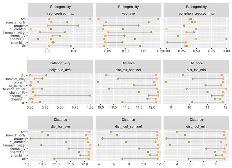
A limitation of our approach is that it requires a large number of high-quality gold standards to train the model, and each source of gold standards will have biases. For example, when we compared the dataset of drug targets from CHEMBL retrospectively mapped to GWAS loci to the manually curated datasets (mainly focused on the closest genes and those with known missense variants), we found that distance and VEP features performed much better in the manually curated datasets (Extended Data Fig. 8), emphasizing the need to curate less-biased datasets. Using varied sources may help mitigate some source-specific biases, but manually curated allele-gene pairs are intrinsically more likely to be close to each other. Future gold-standard training data should represent a range of possible molecular mechanisms. The reliance on large amounts of training data influenced the design of our model. To avoid stratifying gold-standards into smaller subgroups, we trained the model across all diseases at once and using functional data ascertained from different tissues/cell types aggregated into a single feature. This means that the model is not currently able to specifically leverage the tissues/cell types that are most relevant for a given disease.

The outputs of our analyses can be viewed in the Open Targets Genetics portal (https://genetics.opentargets.org), a user-friendly web interface that supports visualization of fine-mapping and L2G scores for individual variants and genes across 133,441 trait-lead variant GWAS associations. The portal also offers other features, including disease-disease and disease-molecular traits colocalization analyses across ~3,600 GWAS summary statistics and 92 tissue and cell type-specific molecular QTL summary statistics to identify traits and diseases that share common genetic susceptibility mechanisms. The portal will regularly be updated with new GWAS summary statistics both from European and non-European ancestries as well as QTLs and functional genomic data from a wider range of tissues and cell types. Planned enhancements include displaying tissue- and cell type-specific enrichments for each trait, using methods such as CHEERS³⁸ that leverage functional annotations. These enrichments will also be used to improve the L2G model by using functional genomics data from tissues that are most relevant to each disease and trait. Our repository of gold-standard gene assignments will be expanded as more evidence arises. In particular, we encourage scientists from the genetics community to contribute to this repository, since having diverse evidence sources can partially address the bias that comes with manually curated sets.

Methods

Summary statistics-based fine mapping

We harmonized summary statistics to ensure that alleles and effect directions were consistent across studies, and we removed variants with low confidence estimates (minor allele count < 10). We identified independently associated loci for each study using Genome-wide Complex Trait Analysis Conditional and Joint Analysis (GCTA-COJO; v1.91.3)²². UK Biobank genotypes down-sampled to 10,000 individuals were used as an LD reference for conditional analysis³⁹. We considered a locus to be independently associated if both marginal and conditional P-values were less than 5 × 10^-8. For each independent locus, we produced a set of summary statistics that are conditional on all other independent loci ±2 Mb from the sentinel variant. Using the conditional set of summary statistics, we computed approximate Bayes factors⁴⁰ from the beta and standard error for each SNP, with a variance prior (W) of 0.15 for quantitative traits and 0.2 for binary traits, and determined variant posterior probabilities (PP) assuming a single causal variant as PP = SNP BF / sum(all SNP BFs) for all SNPs within a ± 500-kb window. We considered any variant with a PP > 0.1% as being in the credible set.

LD-based fine mapping

In addition to the above fine-mapping analysis, we conducted a complementary LD-based approach that allowed us to leverage information from studies that lack full summary statistics. For each independent locus, we identified all variants in LD with the sentinel variant (r ² > 0.5 in ± 500-kb window). LD was calculated in 1000 Genomes phase 3 data⁴¹ by mapping the GWAS study ancestries to the closest superpopulation⁴², taking a sample size weighted-mean of the Fisher Z-transformed correlations in the case of multi-ancestry studies. We then used the Probabilistic Identification of Causal SNPs (PICS) method to estimate the PP that each variant is causal based on the LD structure at each locus²⁴. As above, we kept all variants with PP > 0.1%.

Colocalization analysis

Molecular QTL summary statistics were acquired from the EBI eQTL Catalogue¹⁷, GTEx (v7)¹⁵, eQTLGen¹⁶ and Sun et al. protein QTLs¹⁸. Summary statistics were restricted to be ±1 Mb from the gene transcription start site (TSS). We pre-processed and fine mapped molecular QTL summary statistics using the same method described above for GWAS studies. However, we used less stringent criteria for the inclusion of QTL lead variants, requiring minor allele count ≥ 5 and adjusted for multiple testing using a Bonferroni correction of P < 0.05 / number of variants tested per gene.

For GWAS studies with summary statistics, we performed a colocalization analysis if there was at least 1 variant overlapping between the GWAS and molecular trait 95% credible sets (prior evidence for colocalization). We conducted colocalization of summary statistics using the coloc package (v.3.2-1)²⁸ with default priors. Given that there is prior evidence for colocalization, these parameters will give conservative estimates. As with the fine-mapping pipeline, we used summary statistics conditional on all other independent loci within ±2 Mb and restricted the coloc analysis to a ± 500-kb window around each sentinel variant. A minimum of 250 intersecting variants were required for analysis.

For GWAS studies without summary statistics, we performed an alternative colocalization analysis using the LD-based PICS fine-mapping sets. Colocalization was approximated by taking variants that intersect at pairs of GWAS and molecular trait loci and summing the product of the PPs.

Pre-processing of functional genomics data for L2G prioritization

We used four main classes of evidence to prioritize genes: (i) variant pathogenicity in silico predictions; (ii) colocalization with molecular trait quantitative trait loci (QTL); (iii) chromatin conformation; (iv) linear genomic distance from variant to gene.

We used in silico pathogenicity predictions to estimate the effect of variants on gene transcripts and protein function. First, we incorporated Variant Effect Predictor (VEP)²⁵ transcript consequences. We mapped VEP’s impact ratings of High, Moderate, and Low to scores of 1.0, 0.66, and 0.33 (respectively), and included an additional four consequences (intronic, 5’ UTR, 3’ UTR, nonsense-mediated mRNA decay transcript variants) with a score of 0.1 as we expected them to have predictive value through their functional consequences on mRNA transcription, secondary structure and translation. For each variant-gene pair, we took the maximum score across transcripts. In addition to VEP, we included PolyPhen-2 pathogenicity scores representing the probability that a non-synonymous substitution is damaging⁴³.

Chromatin interaction data were from promoter-capture Hi-C, FANTOM enhancer-TSS correlation, and DNase-hypersensitivity enhancer-promoter correlation. Each of the data points in these datasets is represented as a pair of interacting genomic intervals and an association statistic. We retained interval pairs with one end encompassing an Ensembl gene Transcription Start Site (TSS)⁴⁴ and the other end containing any variant in Gnomad 2.1⁴⁵, resulting in variant-gene pairs with a dataset-specific association statistic.

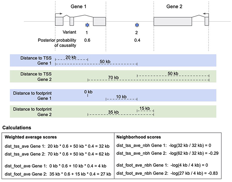
We included two genomic distance metrics as it has been shown that, despite notable contrary exceptions, linear distance is a good predictor of candidate causal genes⁴⁶. First, the distance from each variant to all gene TSSs is included. Second, the distance from each variant to each gene’s footprint is included, where the footprint is any position between the start and end positions of the gene. Variants within a gene’s footprint have a distance of zero. An example of the distance calculation is shown in Extended Data Figure 3. For both metrics, the canonical transcript is used, as defined by Ensembl for protein-coding genes within a ± 500-kb window around each variant.

Derivation of locus-to-gene prioritization features

We next combined our fine-mapping and functional genomics data to create features to prioritize candidate causal genes at each trait-associated locus (locus-to-gene scoring) (Supplementary Table 10).

Except for molecular trait colocalization evidence, each functional genomics dataset is variant-centric, meaning they give variant-to-gene scores. We convert variant-centric scores into locus-to-gene scores by aggregating over credible variants identified through fine mapping. For GWAS studies with summary statistics available, we used ABF credible sets; otherwise, we used LD-based PICS credible sets. We implemented two complementary methods for aggregating over credible sets. First, we took a weighted sum of scores across all variants identified by fine mapping (PP > 0.01%) using PP of causality as weights (Equation 1).

$${weightedScore}_{(study,locus,gene,source,tissue)}={\displaystyle \sum }_{v=i}^n({score}_{(i,gene,source,tissue)}\cdot p{p}_{(study,locus,i)})$$ (Equation 1)

Second, we took the maximum score for any variant in the 95% credible set (Equation 2).

$${maxScore}_{(study,locus,gene,source,tissue)}=max({score}_{(i,gene,source,tissue)})$$ (Equation 2)

Molecular trait colocalization evidence is a locus-centric score. We included both summary statistic derived coloc evidence (Equation 3) and LD-derived colocalization evidence as features.

$${colocSumstatsScore}_{(study,locus,qtltype,tissue,gene)}=maxacrossmolQTLloci({log}_2(\frac{h4}{h3}))$$ (Equation 3)

Each GWAS signal may have colocalization estimates from multiple independent molecular trait signals (each conditional on the others); therefore, we took the maximum score across estimates. Given that evidence against colocalization (h3) cannot be directly estimated without full summary statistics, this term was dropped for the LD-derived colocalization feature (Equation 4).

$${colocLdScore}_{(study,locus,qtltype,tissue,gene)}=maxacrossmolQTLloci({log}_2(h4))$$ (Equation 4)

For functional genomics datasets with measurements in multiple tissues (or cell types), we calculated the locus-level feature for each tissue separately and took the maximum across tissues (Equation 5).

$${feature}_{(study,locus,gene)}=maxacrosstissues({feature}_{(study,locus,tissue,gene)})$$ (Equation 5)

We next wanted to provide the model with information about other genes at each locus (termed the neighbourhood feature). This allows the model to learn whether a given gene has, for example, the highest colocalization score compared to others at the locus. To do this, we divided each feature by the maximum score across genes at that locus (Equation 6).

$${neighbourhoodFeature}_{(study,locus,gene)}=\frac{{feature}_{(study,locus,gene)}}{maxacrossgenes({feature}_{(study,locus,genes)})}$$ (Equation 6)

Curation of a GWAS gold-standard training dataset

We next assembled a repository of published GWAS loci (https://github.com/opentargets/genetics-gold-standards) for which we have high confidence that the gene mediating the association is known. Gold-standard evidence was grouped into four classes: (i) expert curated loci with strong orthogonal evidence or biological plausibility; (ii) drug loci inferred from known drug target-disease pairs; (iii) loci inferred from experimental alteration (e.g. nucleotide editing); (iv) loci inferred from observational functional data (e.g. colocalizing molecular QTLs). We also assigned each gold-standard a confidence rating of high, medium or low depending on our assessment of the strength of supporting evidence.

We started by compiling existing gold-standard examples from the literature. We sourced 227 curated metabolite QTLs from Stacey et al.⁴⁶ and a further 136 loci with strong biological plausibility were curated by Eric Fauman (Supplementary Table 6). We then ascertained 57 genes with “causal” or “strong” observational data from the Type 2 Diabetes Knowledge Portal Effector Genes table, which equates to genes with a confirmed causal coding variant or at least two of the following: (i) a likely causal coding variant, (ii) >1 piece of regulatory evidence, (iii) >1 piece of perturbation evidence⁴⁷. We added a further 48 disease-causal genes curated from the literature. These were mainly GWAS trait-associated loci that were fine-mapped and colocalized with eQTL and epigenomic features in disease-relevant tissues in order to prioritize likely functional variants and their causal genes. These results were then functionally validated using experiments such as reporter assays and CRISPR/Cas9 genome editing.

In addition to literature-sourced loci, gold-standard evidence was generated based on known drug-target-indication associations curated in ChEMBL in clinical trial phase II, III or IV⁴⁸. Drugs that bind a protein complex, rather than a single protein, were removed unless the binding subunit was known. The ChEMBL evidence was combined with the genetics features to identify loci with known drug targets. Gold-standards derived from phase II, III and IV drug targets were assigned a confidence of low, medium and high, respectively. Additionally, confidences were adjusted to indicate the distance of the sentinel variant to the drug target; variant-gene distances of < 500, 250, 100 kb were assigned confidences low, medium and high, respectively.

Duplications were removed from the gold-standard positives (GSPs) list so that GWAS allele-gene pairs never occurred more than once in the training data. The same gene could occur as a GSP more than once if the associated alleles were independent, i.e. if no variants overlapped between their credible sets (using all variants with PP > 0.1%). All non-GSP genes in the training data at the locus (±500 kb) were set as gold-standard negatives (GSNs). GSNs genes were subsequently removed if they had a stringDB score ≥ 0.7 with the GSP at the same locus, the aim being to remove alternative explanations for the association between trait-associated allele and gene. This resulted in a total of 229 GSNs being removed (out of a total of 9,171). A total of 445 GSPs were included in the final training data.

Supervised learning of locus-to-gene features

We used all GWAS loci with high or medium confidence gold-standard evidence (445 loci) to train an XGBoost gradient boosting classifier⁴⁹ using a binary logistic learning objective function. Nested cross-validation (CV) as implemented in scikit-learn was used to maintain independence of the training and test data and to tune hyperparameters. The outer CV consisted of 5 folds split by chromosomes so that each group contained an approximately equal number of GSPs. Within each fold, we used a random parameter search to train 1,000 models, which were assessed using a balanced accuracy metric averaged over 5 randomly split inner folds.

For each group of features included in the main model, we conducted sub-analyzes whereby either only that feature group was included (leave-one-group-in), or everything except that feature group was included (leave-one-group-out). This allowed us to evaluate the relative performance of each feature group individually. Additionally, we output the Relative Importance of each feature as implemented in the XGBoost model⁵⁰.

Model internal validation

Our cross-validation approach produces separate models for each of the 5 outer folds. We evaluated the performance of each model against the remaining 20% of loci not used for training. We used average precision and area under the receiver operator curve (AUC) metrics to assess the classification across the full range of prediction probabilities outputted by the model. We also assess the performance of the model after applying a hard threshold of >0.5 (>50% confidence that the characteristics of the observed locus is consistent with being a gold-standard positive locus).

We compared the relative performance of leave-one-group-in and leave-one-group-out models by calculating the net reclassification improvement (NRI) of loci compared to the full model⁵¹. NRI measures the number of GSP loci that move above the classification threshold (>0.5), compared to GSN that move below, when the model is updated. We also calculate continuous NRI (cNRI), the sum of the percentage of GSPs with classification scores that move in the correct direction vs. GSNs that move in the wrong direction (towards higher scores)⁵².

Model external validation with literature evidence

We benchmarked the L2G assignment against independent gene-disease associations scored by literature mining in the Open Targets Platform. We excluded any publications for studies curated in GWAS Catalog to ensure independence of the training data. We restricted analyses to a subset of 22 prioritized diseases (coronary artery disease, breast carcinoma, prostate carcinoma, acute lymphoblastic leukemia, inflammatory bowel disease, Crohn’s disease, ulcerative colitis, rheumatoid arthritis, osteoarthritis, type 1 diabetes mellitus, hypothyroidism, psoriasis, atopic eczema, asthma, Alzheimer’s disease, Parkinson’s disease, ankylosing spondylitis, celiac disease, gout, multiple sclerosis, systemic lupus erythematosus). For each disease, we constructed a 2 × 2 contingency table of ‘gene prioritized by L2G model (score > 0.5)’ and ‘gene prioritized by Open Targets literature evidence (top decile > 0.52)’. Only genes scored by the L2G model (± 500 kb of a sentinel GWAS variant) were included in the contingency table. We calculated enrichment and statistical significance using Fisher’s exact test.

Enrichment of known drug targets

We calculated drug target enrichment using known target-indication pairs curated in ChEMBL (accessed 25 March 2019). We constructed a single 2 × 2 contingency table pooling across all indications, which consisted of ‘gene prioritized by L2G model (score > 0.5)’ and ‘gene is known target of drug for indication matched to GWAS disease phenotype’. GWAS studies were only included if they could be mapped to a ChEMBL indication (matched using Experimental Factor Ontology) and that indication has a known drug that can be mapped to a protein-coding gene that was scored by the L2G model. Enrichment was calculated by Fisher’s exact test.

Enrichment of Mendelian disease genes

We used the MendelVar⁵³ web server (https://mendelvar.mrcieu.ac.uk/) to annotate Mendelian disease genes, and their corresponding human phenotype ontology (HPO) terms, within a 100-kb window around all independent signals from nine well-powered GWAS traits. We manually identified HPO terms that matched between GWAS and Mendelian diseases and then classified each disease gene as matching or non-matching. In Extended Data Figure 6, we show the distribution of L2G scores for matching and non-matching genes.

Extended Data

Extended Data Figure 1.

Extended Data Figure 2.

Extended Data Figure 3.

Extended Data Figure 4.

Extended Data Figure 5.

Extended Data Figure 6.

Extended Data Figure 7.

Extended Data Figure 8.

Data availability

Our results are freely available through a web portal (genetics.opentargets.org), GraphQL API or through bulk download. GWAS gold-standard genes: github.com/opentargets/genetics-gold-standards.

Code availability

All analysis code is available open source (Apache license) in the following repositories:

• https://github.com/opentargets/genetics-sumstat-data

• https://github.com/opentargets/genetics-finemapping

• https://github.com/opentargets/genetics-colocalisation

• https://github.com/opentargets/genetics-v2d-data

• https://github.com/opentargets/genetics-v2g-data

• https://github.com/opentargets/genetics-l2g-scoring

• https://github.com/opentargets/genetics-gold-standards

• https://github.com/opentargets/genetics-variant-annotation

References

- 1.Hindorff LA, et al. Potential etiologic and functional implications of genome-wide association loci for human diseases and traits. Proc Natl Acad Sci U S A. 2009;106:9362–9367. doi: 10.1073/pnas.0903103106. [DOI] [PMC free article] [PubMed] [Google Scholar]
- 2.Altshuler D, Daly MJ, Lander ES. Genetic mapping in human disease. Science. 2008;322:881–888. doi: 10.1126/science.1156409. [DOI] [PMC free article] [PubMed] [Google Scholar]
- 3.Claussnitzer M, et al. FTO obesity variant circuitry and adipocyte browning in humans. N Engl J Med. 2015;373:895–907. doi: 10.1056/NEJMoa1502214. [DOI] [PMC free article] [PubMed] [Google Scholar]
- 4.Zhu Z, et al. Integration of summary data from GWAS and eQTL studies predicts complex trait gene targets. Nat Genet. 2016;48:481–487. doi: 10.1038/ng.3538. [DOI] [PubMed] [Google Scholar]
- 5.Brænne I, et al. Prediction of causal candidate genes in coronary artery disease loci. Arterioscler Thromb Vasc Biol. 2015;35:2207–2217. doi: 10.1161/ATVBAHA.115.306108. [DOI] [PMC free article] [PubMed] [Google Scholar]
- 6.Fachal L, et al. Fine-mapping of 150 breast cancer risk regions identifies 191 likely target genes. Nat Genet. 2020;52:56–73. doi: 10.1038/s41588-019-0537-1. [DOI] [PMC free article] [PubMed] [Google Scholar]
- 7.Xue A, et al. Genome-wide association analyses identify 143 risk variants and putative regulatory mechanisms for type 2 diabetes. Nat Commun. 2018;9:2941. doi: 10.1038/s41467-018-04951-w. [DOI] [PMC free article] [PubMed] [Google Scholar]
- 8.Okada Y, et al. Genetics of rheumatoid arthritis contributes to biology and drug discovery. Nature. 2014;506:376–381. doi: 10.1038/nature12873. [DOI] [PMC free article] [PubMed] [Google Scholar]
- 9.Fang H, et al. A genetics-led approach defines the drug target landscape of 30 immune-related traits. Nat Genet. 2019;51:1082–1091. doi: 10.1038/s41588-019-0456-1. [DOI] [PMC free article] [PubMed] [Google Scholar]
- 10.Hay M, Thomas DW, Craighead JL, Economides C, Rosenthal J. Clinical development success rates for investigational drugs. Nat Biotechnol. 2014;32:40–51. doi: 10.1038/nbt.2786. [DOI] [PubMed] [Google Scholar]
- 11.Nelson MR, et al. The support of human genetic evidence for approved drug indications. Nat Genet. 2015;47:856–860. doi: 10.1038/ng.3314. [DOI] [PubMed] [Google Scholar]
- 12.Carvalho-Silva D, et al. Open Targets Platform: new developments and updates two years on. Nucleic Acids Res. 2019;47:D1056–D1065. doi: 10.1093/nar/gky1133. [DOI] [PMC free article] [PubMed] [Google Scholar]
- 13.Koscielny G, et al. Open Targets: a platform for therapeutic target identification and validation. Nucleic Acids Res. 2017;45:D985–D994. doi: 10.1093/nar/gkw1055. [DOI] [PMC free article] [PubMed] [Google Scholar]
- 14.Ochoa D, et al. Open Targets Platform: supporting systematic drug-target identification and prioritisation. Nucleic Acids Res. 2021;49:D1302–D1310. doi: 10.1093/nar/gkaa1027. [DOI] [PMC free article] [PubMed] [Google Scholar]
- 15.GTEx Consortium et al. Genetic effects on gene expression across human tissues. Nature. 2017;550:204–213. doi: 10.1038/nature24277. [DOI] [PMC free article] [PubMed] [Google Scholar]
- 16.Võsa U, et al. Unraveling the polygenic architecture of complex traits using blood eQTL metaanalysis. bioRxiv. doi: 10.1101/447367. [DOI] [Google Scholar]
- 17.Kerimov N, et al. eQTL Catalogue: a compendium of uniformly processed human gene expression and splicing QTLs. bioRxiv. doi: 10.1101/2020.01.29.924266. [DOI] [PMC free article] [PubMed] [Google Scholar]
- 18.Sun BB, et al. Genomic atlas of the human plasma proteome. Nature. 2018;558:73–79. doi: 10.1038/s41586-018-0175-2. [DOI] [PMC free article] [PubMed] [Google Scholar]
- 19.Buniello A, et al. The NHGRI-EBI GWAS Catalog of published genome-wide association studies, targeted arrays and summary statistics 2019. Nucleic Acids Res. 2019;47:D1005–D1012. doi: 10.1093/nar/gky1120. [DOI] [PMC free article] [PubMed] [Google Scholar]
- 20.Zhou W, et al. Efficiently controlling for case-control imbalance and sample relatedness in large-scale genetic association studies. Nat Genet. 2018;50:1335–1341. doi: 10.1038/s41588-018-0184-y. [DOI] [PMC free article] [PubMed] [Google Scholar]
- 21.Neale Lab. UK Biobank bulk summary statistics. http://www.nealelab.is/uk-biobank.
- 22.Yang J, et al. Conditional and joint multiple-SNP analysis of GWAS summary statistics identifies additional variants influencing complex traits. Nat Genet. 2012;44:369–375. doi: 10.1038/ng.2213. [DOI] [PMC free article] [PubMed] [Google Scholar]
- 23.Wellcome Trust Case Control Consortium et al. Bayesian refinement of association signals for 14 loci in 3 common diseases. Nat Genet. 2012;44:1294–1301. doi: 10.1038/ng.2435. [DOI] [PMC free article] [PubMed] [Google Scholar]
- 24.Farh KK-H, et al. Genetic and epigenetic fine mapping of causal autoimmune disease variants. Nature. 2015;518:337–343. doi: 10.1038/nature13835. [DOI] [PMC free article] [PubMed] [Google Scholar]
- 25.McLaren W, et al. The Ensembl Variant Effect Predictor. Genome Biol. 2016;17:122. doi: 10.1186/s13059-016-0974-4. [DOI] [PMC free article] [PubMed] [Google Scholar]
- 26.Michailidou K, et al. Association analysis identifies 65 new breast cancer risk loci. Nature. 2017;551:92–94. doi: 10.1038/nature24284. [DOI] [PMC free article] [PubMed] [Google Scholar]
- 27.Kawase T, et al. PH domain-only protein PHLDA3 is a p53-regulated repressor of Akt. Cell. 2009;136:535–550. doi: 10.1016/j.cell.2008.12.002. [DOI] [PubMed] [Google Scholar]
- 28.Giambartolomei C, et al. Bayesian test for colocalisation between pairs of genetic association studies using summary statistics. PLoS Genet. 2014;10:e1004383. doi: 10.1371/journal.pgen.1004383. [DOI] [PMC free article] [PubMed] [Google Scholar]
- 29.Burgess S, et al. Guidelines for performing Mendelian randomization investigations. Wellcome Open Research. 2020;4:186. doi: 10.12688/wellcomeopenres.15555.1. [DOI] [PMC free article] [PubMed] [Google Scholar]
- 30.Surendran S, et al. An update on vitamin B12-related gene polymorphisms and B12 status. Genes Nutr. 2018;13:2. doi: 10.1186/s12263-018-0591-9. [DOI] [PMC free article] [PubMed] [Google Scholar]
- 31.Todd JA. Evidence that UBASH3 is a causal gene for type 1 diabetes. Eur J Hum Genet. 2018;26:925–927. doi: 10.1038/s41431-018-0142-2. [DOI] [PMC free article] [PubMed] [Google Scholar]
- 32.de Lange KM, et al. Genome-wide association study implicates immune activation of multiple integrin genes in inflammatory bowel disease. Nat Genet. 2017;49:256–261. doi: 10.1038/ng.3760. [DOI] [PMC free article] [PubMed] [Google Scholar]
- 33.Mosnier J-F, et al. ADAM15 upregulation and interaction with multiple binding partners in inflammatory bowel disease. Lab Invest. 2006;86:1064–1073. doi: 10.1038/labinvest.3700465. [DOI] [PubMed] [Google Scholar]
- 34.Jung I, et al. A compendium of promoter-centered long-range chromatin interactions in the human genome. Nat Genet. 2019;51:1442–1449. doi: 10.1038/s41588-019-0494-8. [DOI] [PMC free article] [PubMed] [Google Scholar]
- 35.Andersson R, et al. An atlas of active enhancers across human cell types and tissues. Nature. 2014;507:455–461. doi: 10.1038/nature12787. [DOI] [PMC free article] [PubMed] [Google Scholar]
- 36.Thurman RE, et al. The accessible chromatin landscape of the human genome. Nature. 2012;489:75–82. doi: 10.1038/nature11232. [DOI] [PMC free article] [PubMed] [Google Scholar]
- 37.Visscher PM, Brown MA, McCarthy MI, Yang J. Five years of GWAS discovery. Am J Hum Genet. 2012;90:7–24. doi: 10.1016/j.ajhg.2011.11.029. [DOI] [PMC free article] [PubMed] [Google Scholar]
- 38.Soskic B, et al. Chromatin activity at GWAS loci identifies T cell states driving complex immune diseases. Nat Genet. 2019;51:1486–1493. doi: 10.1038/s41588-019-0493-9. [DOI] [PMC free article] [PubMed] [Google Scholar]
- 39.Bycroft C, et al. The UK Biobank resource with deep phenotyping and genomic data. Nature. 2018;562:203–209. doi: 10.1038/s41586-018-0579-z. [DOI] [PMC free article] [PubMed] [Google Scholar]
- 40.Wakefield J. Bayes factors for genome-wide association studies: comparison with P-values. Genet Epidemiol. 2009;33:79–86. doi: 10.1002/gepi.20359. [DOI] [PubMed] [Google Scholar]
- 41.1000 Genomes Project Consortium et al. A global reference for human genetic variation. Nature. 2015;526:68–74. doi: 10.1038/nature15393. [DOI] [PMC free article] [PubMed] [Google Scholar]
- 42.Morales J, et al. A standardized framework for representation of ancestry data in genomics studies, with application to the NHGRI-EBI GWAS Catalog. Genome Biol. 2018;19:21. doi: 10.1186/s13059-018-1396-2. [DOI] [PMC free article] [PubMed] [Google Scholar]
- 43.Adzhubei IA, et al. A method and server for predicting damaging missense mutations. Nat Methods. 2010;7:248–249. doi: 10.1038/nmeth0410-248. [DOI] [PMC free article] [PubMed] [Google Scholar]
- 44.Zerbino DR, et al. Ensembl 2018. Nucleic Acids Res. 2018;46:D754–D761. doi: 10.1093/nar/gkx1098. [DOI] [PMC free article] [PubMed] [Google Scholar]
- 45.Karczewski KJ, et al. The mutational constraint spectrum quantified from variation in 141,456 humans. Nature. 2020;581:434–443. doi: 10.1038/s41586-020-2308-7. [DOI] [PMC free article] [PubMed] [Google Scholar]
- 46.Stacey D, et al. ProGeM: a framework for the prioritization of candidate causal genes at molecular quantitative trait loci. Nucleic Acids Res. 2019;47:e3. doi: 10.1093/nar/gky837. [DOI] [PMC free article] [PubMed] [Google Scholar]
- 47.Type 2 Diabetes Knowledge Portal. 2019 http://www.type2diabetesgenetics.org/gene/effectorGeneTable.
- 48.Gaulton A, et al. The ChEMBL database in 2017. Nucleic Acids Res. 2017;45:D945–D954. doi: 10.1093/nar/gkw1074. [DOI] [PMC free article] [PubMed] [Google Scholar]
- 49.Chen T, Guestrin C. XGBoost; Proceedings of the 22nd ACM SIGKDD International Conference on Knowledge Discovery and Data Mining - KDD ‘16; 2016. [DOI] [Google Scholar]
- 50.Friedman JH. Greedy function approximation: A gradient boosting machine. Ann Stat. 2001;29:1189–1232. [Google Scholar]
- 51.Pencina MJ, D’Agostino RB, D’Agostino RB, Vasan RS. Evaluating the added predictive ability of a new marker: from area under the ROC curve to reclassification and beyond. Stat Med. 2008;27:157–172. doi: 10.1002/sim.2929. [DOI] [PubMed] [Google Scholar]
- 52.Pencina MJ, D’Agostino RB, SrSteyerberg EW. Extensions of net reclassification improvement calculations to measure usefulness of new biomarkers. Stat Med. 2011;30:11–21. doi: 10.1002/sim.4085. [DOI] [PMC free article] [PubMed] [Google Scholar]
- 53.Sobczyk MK, Gaunt TR, Paternoster L. MendelVar: gene prioritisation at GWAS loci using phenotypic enrichment of mendelian disease genes. Bioinformatics. 2021;37:1–8. doi: 10.1093/bioinformatics/btaa1096. [DOI] [PMC free article] [PubMed] [Google Scholar]
Associated Data
This section collects any data citations, data availability statements, or supplementary materials included in this article.
Supplementary Materials
Data Availability Statement