Towards the biogeography of prokaryotic genes

Abstract

Microbial genes encode the majority of the functional repertoire of life on earth. However, despite increasing efforts in metagenomic sequencing of various habitats^1–3, little is known about the distribution of genes across the global biosphere, with implications for human and planetary health. Here we constructed a non-redundant gene catalogue of 303 million species-level genes (clustered at 95% nucleotide identity) from 13,174 publicly available metagenomes across 14 major habitats and use it to show that most genes are specific to a single habitat. The small fraction of genes found in multiple habitats is enriched in antibiotic-resistance genes and markers for mobile genetic elements. By further clustering these species-level genes into 32 million protein families, we observed that a small fraction of these families contain the majority of the genes (0.6% of families account for 50% of the genes). The majority of species-level genes and protein families are rare. Furthermore, species-level genes, and in particular the rare ones, show low rates of positive (adaptive) selection, supporting a model in which most genetic variability observed within each protein family is neutral or nearly neutral.

Metagenomic shotgun sequencing enables quantification of molecular functions in environmental samples, often enabled by gene catalogues, which combine information from multiple local assemblies⁴. Such catalogues have been used for the human gut⁴, as well as for other host-associated^5,6 and environmental habitats^1,3. More recently, increased sequencing depth has enabled more complete genome assembly (metagenome-assembled genomes (MAGs)), providing contextual information on genes⁷. However, despite the increasing amount of information on genes and their known ability to cross species and habitat barriers (affecting human health⁸), a comprehensive assessment of the gene distribution across the global biosphere has not yet been performed.

The Global Microbial Gene Catalogue

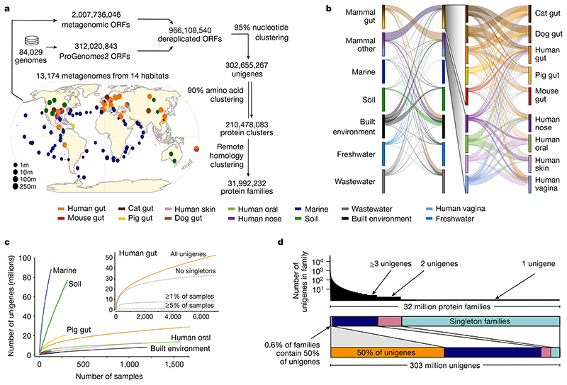
Here we integrate metagenomes and complete genomes, surveying prokaryotic genes across habitats to gain an understanding of the global distribution of genes and the molecular functions they encode. We collated data from 14 habitats (both host-associated and environmental; Fig. 1) in an integrated, consistently processed, non-redundant Global Microbial Gene Catalogue (GMGCv1).

Fig. 1. Global Microbial Gene Catalogue, version 1.

a, Metagenomes from 14 different habitats (marker size represents total number of short reads) were assembled and ORFs were extracted. These, combined with ORFs from proGenomes2, were clustered to form species-level unigenes, protein clusters and protein families (Methods). b, Sharing of unigenes between habitats is minimal, with the exception of sharing between mammalian gut microbiota. The width of each ribbon represents the average abundance of the shared genes in the habitat on the left. The widest ribbon connects the cat gut to the human gut and represents the fact that 58.0% of the reads in cat gut microbiomes map to genes shared with the human gut. c, The unigene accumulation curves show that some habitats reach diminishing returns per sample, whereas others (for example, marine and soil) are still under-sampled (Extended Data Fig. 1). Inset, for the human gut, the curve saturates for the most prevalent genes. However, rare unigenes, including sample-specific ones, are still being discovered. d, The largest protein family contains 73,979 unigenes. However, the size distribution is long-tailed and half of all unigenes are contained in only 203,431 (0.6%) families (those containing ≥239 species-level unigenes), while 80% of protein families consist of only one or two genes, encompassing slightly less than 8% of the total unigene pool.

GMGCv1 was derived from 13,174, publicly available, high-quality metagenomes (Methods, Supplementary Tables 1, 2). The underlying samples were annotated with their respective habitat by semi-manual curation. We assembled contigs and predicted open reading frames (ORFs) from each metagenome, resulting in 2,007,736,046 ORFs (Methods, Extended Data Fig. 1, Supplementary Table 3). To broaden the coverage of our catalogue, we included 312,020,843 ORFs from 84,029 high-quality genomes from the proGenomes2 database⁹. Using a graph-based redundancy removal algorithm (Methods), the resulting 2,319,756,889 sequences were, as in previous habitat-specific gene catalogues^1,4–6, clustered at 95% nucleotide identity–a threshold that roughly corresponds to species boundaries¹⁰ (Extended Data Fig. 2)–resulting in 302,655,267 clusters. A single sequence from each cluster was retained, representing all the nucleotide variants at 95% nucleotide identity–this corresponds to one copy of a particular gene per species, which is hereafter referred to as the ‘unigene’.

To be able to generalize on global gene distribution properties, we also grouped sequences more broadly using a homology-based clustering approach¹¹, on the basis of statistically significant sequence similarity (e-value < 10⁻³; Methods) and four additional thresholds of amino acid identity (>90%, >50%, >30% and >20%). Requiring a minimum of 90% identity represents a strict, yet common, cut-off in protein databases12 and led to 210,478,083 unique protein clusters, while considering all statistically significant homologues with at least 20% amino acid identity resulted in 31,992,232 very broadly defined protein families.

An inevitable limitation of current metagenomics is that most assembled contigs are short relative to the size of ORFs, leading to many incomplete ORFs. As some analyses may benefit from a stricter emphasis on the quality of individual sequences (at the cost of lower coverage) and as 68.5% of the unigenes in GMGCv1 are predicted to be incomplete ORFs, we created a version of the catalogue including only complete ORFs and also built operationally defined protein families at different stringencies from them (https://gmgc.embl.de).

Both the inclusion of incomplete ORFs and the different operational protein family definitions can potentially affect functional and phylogenetic interpretations. Therefore, while we focus here on the broadest operational protein family definition (statistically significant sequence similarity, with at least 20% amino acid identity, including all ORFs), all our observations are robust across the several thresholds tested as well as to the inclusion of incomplete ORFs (Supplementary Table 4).

The majority of species-level unigenes in GMGCv1 were included in a tiny fraction of large protein families (the 0.6% largest protein families contain half of the species-level unigenes (Fig. 1d)). As a case in point for the robustness of the results with regard to parameter definitions, this fraction changes only slightly when exclusively considering complete ORFs (0.5%) or choosing a stricter definition of protein family (for example, 0.9% at the 50% clustering cut-off; Supplementary Table 4). The large amount of genetic diversity observed in GMGCv1 is thus mostly owing to diversification within protein families, rather than de novo creation of genes.

We next attempted to put the genes into genomic context and produced 278,629 MAGs. Even without removing low-quality assemblies (Methods, Supplementary Table 5), these MAGs contain only 40 million species-level unigenes, compared with the 303 million in the full catalogue. Yet–in agreement with previous reports⁷–this MAG subset is sufficient for mapping short reads from well-studied habitats at high rates, as MAGs preferentially capture higher-abundance genes (in the well-studied human gut metagenome, 95.3% of reads map to MAGs, but 42.5% of unigenes do not; Extended Data Figs. 3, 4).

Most genes are habitat-specific

Whereas MAGs are usually built per sample or per habitat, the global microbial gene catalogue enabled us to identify genes that are shared between habitats. As the species-level unigenes represent multiple sequences (with nucleotide identity greater than 95%), they may represent genes from multiple habitats (‘multi-habitat genes’). These could be contained in species thriving in multiple habitats or be part of mobile elements, that is, genes that can be transferred horizontally between genomes and across habitat boundaries.

Only 18,145,135 species-level unigenes (5.8% of the total, P < 10⁻³⁸, permutation test; Methods) are multi-habitat genes (Fig. 1b, Extended Data Fig. 5). This is consistent with findings that species tend to adapt to their environments¹³ and that in host-associated microbiomes, conspecific strains contain host-specific genes^6,14.

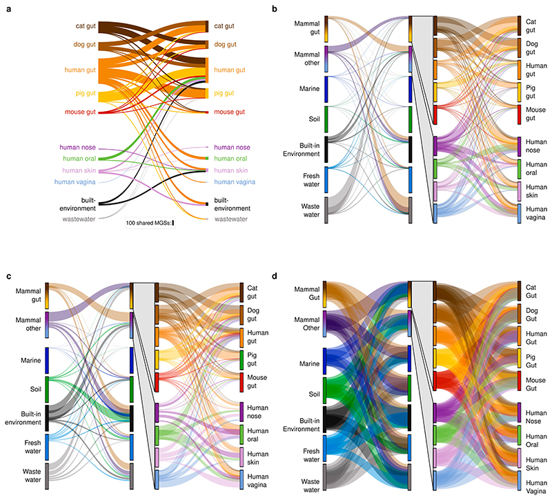
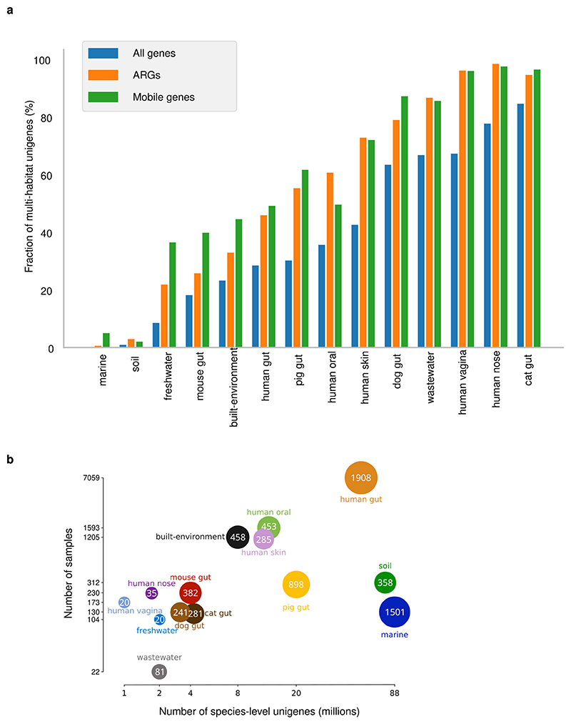
To disentangle the mechanisms by which genes traverse habitat boundaries (that is, with entire species or with mobile elements), we first looked for unigenes associated with mobile elements (Methods) and found that they are indeed more than twice as likely to be in multiple habitats (156,738 out of 1,182,749 (13.3%), P < 10⁻³⁸, Fisher’s exact test; Extended Data Fig. 6) than the average unigene (5.8%). Antibiotic-resistance genes (ARGs)–which are thought to be frequent cargo of mobile elements⁸–were, also as expected, more likely than other unigenes to be present in multiple habitats (329,857 out of 3,208,187 ARGs (10.3%) P < 10⁻³⁸, Fisher’s exact test; Extended Data Fig. 6, Methods). To quantify species overlap between habitats, taking into account that many species are not yet known, we constructed metagenomic species (MGSs) for each habitat (Methods) as proxies for species¹⁵ with reliable habitat information. Overall, 7,443 MGSs were built, out of which only 1,099 are shared between habitats, consistent with the sharing patterns observed for individual unigenes (Extended Data Fig. 5, cf. Fig. 1b). As expected, species are more likely to be shared between similar environments (Extended Data Fig. 7); for example, the different mammalian gut habitats share many MGSs (786 of the 1,099 that are shared).

Richness patterns are habitat-specific

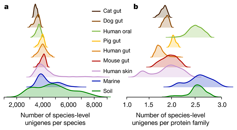
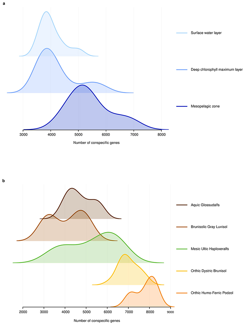
To investigate the presence of conspecific genes in each sample, we used the richness of universal, single-copy genes¹⁶ to measure taxonomic richness and compared it to overall unigene richness (Methods). We observed distinct average number of species-level unigenes per species in each sample (Fig. 2a, P < 10⁻³⁸, Kruskal–Wallis test). The marine and soil environments show a mixture of multiple sub-patterns. In the case of the marine samples, these sub-patterns correspond to distinct ocean depths, especially when comparing shallow samples to those collected in deeper water that is inaccessible to sunlight¹, whereas the differences in soil environments follow differences in acidity and moisture (Extended Data Fig. 8). Thus, the number of unigenes per species present in a metagenome emerged as an identifying feature of a well-defined habitat.

Fig. 2. The number of conspecific genes (gene pool per species) and the functional redundancy in each metagenome show significantly less variation within than between habitats.

a, Density (smoothed histogram using a Gaussian kernel with the width automatically determined (Methods)) of the number of conspecific genes in each sample, by habitat, shows that the largest per-sample pangenomes are present in environmental samples rather than in host-associated habitats. b, Density of the number of unigenes for each protein family (a proxy for functional redundancy) detected in each sample, per habitat, shows clear differences between habitats. The protein family richness is highly correlated in the well-studied human gut habitat to the stricter orthologue-richness estimate obtained using eggnog-mapper2¹⁷ and extends to all habitats (Methods).

To test whether the observed unigene richness was driven primarily by communities containing multiple orthologous unigenes (assumed to be performing the same metabolic function¹⁷) or a variety of functional groups, we calculated the ratio of protein family richness to species-level unigene richness as a proxy for functional redundancy, and observed clear differences between habitats (Fig. 2b). We further tested the habitat specificity by building a classifier that predicts the habitat of each sample using only four descriptors (taxonomic, phylogenetic, unigene and protein family richness, after rarefaction to control for differences in sequencing depth; Methods). By cross-validation, we estimated the accuracy of this classifier across the 14 habitats at 86.1% (controlling for the class size imbalance by downsampling habitats to a maximum of 200 samples, so the largest habitats represent at most 11.8% of the dataset; Methods). Functional redundancy, whereby multiple organisms encode the same function, has been described in multiple environments¹⁸. Although it falsifies simplistic models in which each metabolic niche is occupied by a single species, there is still no consensus on the processes that explain it or its implications¹⁸. From our data, we conclude that the functional redundancy within each environment is tightly connected to the habitat within which the community develops, consistent with observations on pangenomes¹⁹. Thus, general models of functional redundancy will need to incorporate habitat-specific parameters.

Most genes are rare

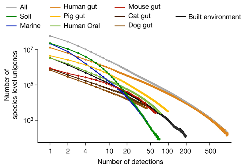
Having established that functional redundancy and the majority of genes are habitat-specific, we investigated how frequent unigenes are in metagenomes. We observed that the prevalence of species-level unigenes follows a power law, with differing parameters for each habitat (Fig. 3), clearly showing that most genes have low prevalence. In fact, if we consider genes detected in 10 or fewer samples (out of 13,174 analysed, so less than 0.1%) as rare genes, then most unigenes in the GMGCv1 are rare (54.7% of genes, with similar results when considering broader clustering levels; Extended Data Fig. 9, Supplementary Table 4).

Fig. 3. Most genes are rare.

Histograms of gene prevalence are roughly linear on a log-log scale, as predicted from neutral or nearly neutral evolution models (Methods).

These frequency distributions in the form of power laws are expected under the assumption of neutral (or nearly neutral) evolution²⁰ and describe our data well (for the human gut, the Pearson correlation between theoretical fit and observed data for unigenes is 0.997, P = 9.7 × 10⁻¹¹², n = 7,059; Supplementary Table 6, Methods).

In agreement with this model, the vast majority of protein families (designed to include distant homologues; Methods), consist of rare, low-abundance clusters around species-level unigenes with no further homologues (Fig. 1d, Extended Data Fig. 10). Genes without detectable homologues are expected to have little (if any) effect on the fitness of the organisms–as has been observed for fully sequenced genomes²¹ and should hold true in the environmental context.

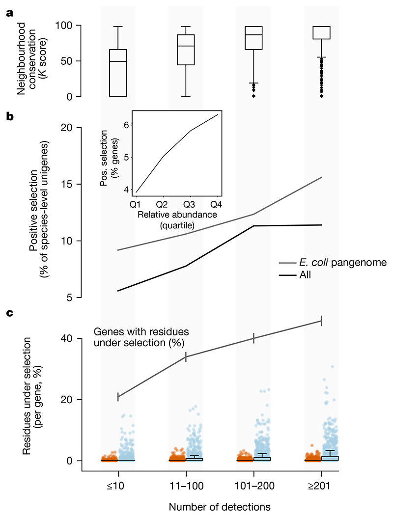
Owing to the operon structure, functionality can be inferred by the co-occurrence of neighbouring genes²²–we therefore measured the conservation of gene order and pathway neighbourhood across prevalence classes. Rare species-level unigenes appear indeed less functionally interacting than prevalent ones (Fig. 4a), consistent with rare genes being under fewer evolutionary constraints.

Fig. 4. Rare unigenes are under lower selection pressure.

a, The operon structure is more frequently preserved in prevalent genes (estimated using genetic neighbourhood relations (Methods)). b, The fraction of unigenes under detectable positive selection (using the HyPHY aBS-REL method (Methods)) increases with the number of detections. This also holds in the E. coli pangenome. Inset, due to the correlation of prevalence and abundance, less-abundant genes are under lower selective pressure than more highly abundant ones (data are split into relative abundance quartiles). c, The E. coli pangenome is the only one of sufficient size to test for selection per site. High-prevalence genes within the E. coli pangenome show evidence of stronger negative (blue) and positive (red) selection than rare genes (fewer detections in GMGCv1) per site. Box plots and dots show the fraction of residues under significant selection per unigene over the total alignment length (n = 4,167 for each category). The grey line shows the fraction of genes with at least one residue under selection (error bars indicate s.e.m.). Despite this overall trend we observed evidence of strong selection in a few rare E. coli genes. For example, we found instances of the UDP-glucose 6-dehydrogenase gene, which contributes to antibiotic resistance, with evidence of selection despite being observed in only six samples. Box plots show the median and the quartiles, with whiskers extending to the furthest data points (excluding outliers, detected using Tukey’s rule).

We then investigated whether our data are compatible with a neutral model of evolution by analysing sequence variation. Neutrality would imply that most observed genetic differences have (almost) no effect on fitness and therefore are not due to adaptation (positive selection) to particular niches, although purifying (negative) selection may still be active²³. As selection operates differently between protein families²⁴, we tested for positive (adaptive) selection within each of our protein families (Methods). We found that the vast majority of unigenes does not show evidence of positive selection (Fig. 4b).

Yet, we observed that rare unigenes are much less likely (4%) than prevalent ones (up to 10%) to be adaptive (Fig. 4b). To guard against possible confounding effects of differences in evolutionary speed and prevalence between species as well as for possible technical issues, we used only unigenes from 5,126 well-annotated Escherichia coli genomes included as part of GMGCv1 and obtained a very similar correlation of increased positive selection and gene prevalence (Fig. 4b). Moreover, the available number of E. coli genomes in GMGCv1 was sufficient to test for selection at each site, and indeed this showed that sites in rare E. coli unigenes were under less detectable selective pressure than those in more prevalent ones (Fig. 4c).

Within a single genome, however, most genes are neither under low selection pressure²⁵ nor rare. In the 5,126 E. coli genomes, only 2.8% ± 1.7% (mean ± s.d.) of the genes in each genome are rare (that is, they occur in 10 or fewer of the metagenomes in our collection). Yet the reservoir of E. coli strains in different habitats is vast, corresponding to the observation that the pangenome of E. coli, like that of most other bacteria, is open²⁶, and thus its genomes will collectively contain a huge number of rare genes.

Although we cannot quantify the relative contribution of ecological and evolutionary processes to the observed patterns²⁷ or prove nearly neutral evolution for rare genes, as our sampling and sequencing depth is biased against very rare genes, the observed correlations point to such a model and indicate that we might still be underestimating the excess of rare genes.

Thus, as costs of sequencing continue to decrease, it seems feasible that we will be able to capture all abundant prokaryotic species on earth, as this goal appears almost achieved for well-studied habitats such as the human gut. Given our data, this even seems feasible for habitats, such as soil, with very high biodiversity. However, owing to the vast amount of rare, habitat-specific and perhaps even region-specific genes, as well as a probable turnover process of de novo gene creation, modification and extinction, considerable parts of the global gene pool will probably never be captured.

Methods

Selection of genomes and metagenomes

Metagenomes were downloaded from the European Nucleotide Archive (ENA)^{1,5,15,28–59}. Only samples that were public on 1 January 2017 were used. Metagenomes were identified using the following two criteria: (1) samples tagged with a taxonomic ID that is either 408169, the taxonomic ID for metagenome, or a taxonomic ID that is a descendent of 408169 in the taxonomic tree; and (2) experiments where the library source field was set to “METAGENOMIC”. Samples containing at least 1 million reads, with an average length of at least 75 base pairs, and having been sequenced on an Illumina instrument, were selected for further analysis. Samples were then grouped by ENA project and all projects with at least 100 samples were considered. Manual inspection led to the rejection of five studies as they either contained eukaryotic samples or consisted of amplicon sequences.

To broaden the set of biomes under study, cat gut and soil metagenomes were manually added. These samples fulfil the quality criteria above (over 1 million reads, >75 bp per read, on average), but are contained in projects with fewer than 100 samples.

This selection and data download is implemented by the Python scripts in the fetch-data/ directory of the supplementary software package, which rely on the requests package. The resulting set of samples is listed in Supplementary Table 1. Based on further analyses, 369 samples were found to be misannotated and to consist of amplicon data. Thus, while they were used in the construction of the catalogue, they were not used in the rest of the analyses in this work.

Genomes were selected as in the proGenomes2 database⁹, by collecting an updated set of high quality genomes from the NCBI database.

The map in Fig. 1a shows the geographical distribution of samples. It was created using R⁶⁰ and the package maptools (version 1.1.0).

Contig assembly and ORF prediction

The reads were processed using NGLess⁶¹, discarding short reads (less than 60 bp), after trimming positions with quality <25. Filtered reads were assembled into contigs with Megahit⁶² (using default parameters for metagenomics) and open read frames (ORFs) were predicted with MetaGeneMark⁶³. These steps were performed using the NGLess⁶¹ script assemble/assemble.ngl in the supplementary software package.

Non-redundant gene catalogue construction

A non-redundant unigene catalogue was built in a four-step process.

Step 1: using rolling hashes, exact matches are found and genes which are perfectly contained in another gene are removed. This step is performed by the Jugfile⁶⁴ and the other scripts in the directory redundant100/ of the supplementary software package.

Step 2: using DIAMOND⁶⁵, all genes are compared against each other.

Step 3: the matches resulting from the previous step are filtered (in nucleotide space) so that only ‘representable’ relationships are kept. Namely, A is considered representable by B if there is a sequence A’ such that A’ is a substring of B and the edit distance from A to A’ is ≤5% of the length of A. When the lengths are identical (or similar), this definition corresponds to the species-level 95% nucleotide identity criterion (Extended Data Fig. 2a). When A is a fragment of B (even with minor changes), however, then only B is kept. The result of this step is a graph where each vertex is an input gene sequence and directed edges correspond to representable relationships.

Step 4: select a dominant vertex set. A dominant vertex set, D, is a set of vertices such that all vertices in the original graph are either (1) contained in D, (2) represented by a gene that is contained in D. This step is solved using a greedy approach: starting with the empty set, iteratively add vertices to the output choosing, at each step, the vertex whose addition would most increase the number of represented sequences. Ties are broken in an arbitrary, but reproducible manner, by using the order of the sequences in the input file as the fallback criterion.

Steps 2–4 are performed by the code in the cluster-genes directory in the supplementary software package.

Quality control of the GMGCv1

Although a large number of unigenes (189,105,503) could only be assembled in a single sample, 74.9% of these assembly singletons were subsequently detected in multiple samples by read mapping (see ‘Metagenomic annotation and profiling’ for details on detection). Similarly, despite the fact that a large fraction of unigenes are incomplete ORFs, at least 91.7% of them are merged into protein families. This includes 83.2%, which cluster into a protein family that includes at least one complete unigene (that is, they are homologous to a complete ORF sequence, so are as real as those) and 8.5% which form small protein families of their own (which also considerably increases the likelihood that they represent real genes).

The unigene resulting catalogue was screened for potential chimeras by aligning it to Uniprot using DIAMOND (parameters: blastp -c 1 -b 4.0). Genes which had (at least) two alignments with >70% amino acid identity with an overlap of fewer than 10 amino acids were considered potential chimeras. Only 920,579 unigenes met this criterion.

To further check the effect of including incomplete ORFs in the catalogue, we checked whether there was extensive overlap of fragments at gene ends, as would be expected if multiple incomplete ORFs originate from a single real sequence that we failed to assemble completely. However, we reasoned that if the problem was extensive, we would frequently observe overlaps at the edges of fragments. To directly test this hypothesis, we aligned a randomly selected set of unigenes back to the full catalogue (using a combination of DIAMOND⁶⁵ in amino acid space to pre-filter and full Smith–Waterman nucleotide alignments to obtain the final result). We counted how often we could find another gene that overlapped (at ≥95% nucleotide identity) with the query at one of its edges. Eight per cent of unigenes had such an edge overlap. The presence of overlaps is not, by itself, sufficient to conclude that we have extraneous unigenes. It is not uncommon that pairs of unigenes have internal regions of high identity even though the sequences as a whole are still above the threshold. Although this analysis does not completely exclude the possibility that genes generate non-overlapping fragments (particularly, if they start at opposite ends), we could not find evidence of widespread fragmentation.

We also checked whether incomplete ORFs show different behaviour in prevalence. For this, we compared the prevelance of ORFs that are adjacent in a metagenomic contig. Incomplete ORFs are, in general, less prevalent (which is natural, as the more often a sequence is observed, the more likely it is that it will be assembled into the complete gene). However, the overall correlation (Spearman r) in prevalence between adjacent ORFs on a contig (technically, between the unigenes that are representing them) is very similar: complete/complete: 0.46; complete/fragment: 0.48; fragment/fragment: 0.49.

To assess possible human contamination, the catalogue was split into files containing 50,000 sequences and aligned with blastn (nucleotide–nucleotide BLAST + 2.7.1) against a human genome reference (GRCh38. p10) containing genomic, cdna and 45S rRNA regions. An e-value of 0.00001 was used. Results were then processed and alignments with spans of <100 nucleotides were discarded if this corresponded to less than 2/3 of the length of the query sequence. Finally, we considered the highest identity across all alignments of every unigene and removed unigenes with ≥97% identity from the catalogue.

AntiFAM⁶⁶ was used to detect spurious ORFs and reported only 37,428 unigenes (0.012%) as matching its database of known false positives.

Metagenome-assembled genomes construction

MAGs were built using Metabat2⁶⁷ using default parameters, by binning on the contigs described above from per sample mappings obtained with BWA⁶⁸. This resulted in a total of 278,629 bins. Genome statistics were estimated using the lineage workflow of checkM⁶⁹ and they are provided for all bins in Supplementary Table 5. Genomes are classified into high, medium, or low quality following MIMAG cut-offs⁷⁰.

Metagenomic species construction

MGSs were identified for each biome using co-abundance clustering¹⁵. Only complete unigenes that were observed in at least 3 samples were clustered. A Pearson correlation coefficient above 0.9 was used as cut-off and the canopy profiles were calculated sample-wise as the 75th percentile abundance across all genes. Co-abundant gene clusters were filtered based on their size, inter-quartile GC range, presence of marker genes, and taxonomy. The resulting 7,443 clusters contained more than 500 genes and were called MGSs. MGSs where at least 80% of the genes could be annotated to a single species with 95% sequence identify were said to be of that species. MGSs with inconsistent taxonomy (>10% ambiguity at any given taxonomic level) were discarded. MGSs with an inter-quartile GC above 10% were also discarded. MGSs that were annotated to Bacteria and Archaea at kingdom level, and which contained fewer than 6 marker genes, were also removed.

Estimation of mapping rates to GMGCv1 and reference genomes

To estimate the quantity of ‘microbial dark matter’ for each habitat, we built a non-redundant catalogue based exclusively on the subset of ORFs from the sequenced genomes used in the global catalogue, resulting in 44,098,640 non-redundant unigenes. Aligning the metagenomic reads to this collection revealed that, for certain habitats, sequenced genomes already capture most of the biodiversity, for example, for human gut samples, on average 80.3% of the short reads in the samples can be aligned to sequenced genomes (Extended Data Fig. 3a), a result that is consistent with previous work⁷¹. However, even for the human gut, there are samples that are not well represented by sequenced genomes only, particularly samples from less well-studied, lower-income countries (Extended Data Fig. 3b, c).

Protein family cluster calculation

For computing protein family clusters we used standard MMseqs2¹³ (version fd3db05699decf550f428782e1b382a9b7f490e1) settings with an additionally required amino acids identity threshold of 50%, 30% or 20% and a minimum sequence coverage of 50% (keeping the default minimum e-value threshold of 10⁻³). The parameters used were --min-seq-id 0.2 -c 0.5 -cov-mode 2 -cluster-mode 0 (where 0.2 was replaced by 0.3 and 0.5, for 30% and 50% identity, respectively). Supplementary Table 4 provides summary statistics on the results of this clustering process.

Protein clusters were done similarly, with a minimum identity threshold of 90% and a minimum sequence coverage of 90%. The parameters used were -min-seq-id 0.9 -c 0.9 -cov-mode 1 -cluster-mode 2.

Taxonomic predictions

Taxonomic predictions were obtained by a combination of three approaches: (1) unigenes that cluster at <95% (nucleotide identity) with sequences from a single species were assigned to that species. For the remaining unigenes, (2) the best hit (as determined by DIAMOND) to the full Uniprot database predicted the superkingdom (Bacteria/Archaea/Eukarya/Viruses). (3) For unigenes predicted as bacterial or archaebacterial in the previous step, the dual-BLAST least common ancestor approach⁷² (using the amino acid representation and DIAMOND as an alternative to BLAST) was used to determine the final prediction. Species-level assignments from this method were converted to genus level.

This method assigned a prediction to 78.4% of GMGCv1 unigenes at levels ranging from species to domain of life (Extended Data Fig. 2). Of these unigenes, 94.6% were classified as bacterial genes, while 2.7% were archaeal, 1.7% were eukaryotic and 0.9% were viral genes.

Estimation of within-species and within-genus nucleotide identity thresholds

Genes were annotated in Prokka⁷³. Blastn (nucleotide–nucleotide BLAST 2.2.29+) searches were performed on 107 species (specI clusters) which belong to 32 genera. Each specI cluster had at least 10 genomes. SpecI clusters that contained more than 20 genomes were randomly down-sampled to 20 genomes). We used all genes in each genome for blastn searches against other genomes in a specI cluster or between specI clusters from the same Genus. Nucleotide identity in Extended Data Fig. 2a is the average of all identities of gene matches in the pair of genomes. In total we performed 14,686 pairwise genome-comparisons within specI clusters and 51,368 comparisons between specI clusters within genera.

Estimation of amino acid identity within orthologues

Average amino acid identity was computed for the clusters in eggNOG 5⁷⁴ corresponding to previously characterized 40 universal marker genes that span bacteria and archea¹³, namely: COG0098, COG0091, COG0186, COG0088, COG0200, COG0202, COG0184, COG0100, COG0049, COG0256, COG0097, COG0522, COG0090, COG0048, COG0495, COG0185, COG0102, COG0541, COG0096, COG0215, COG0081, COG0087, COG0201, COG0080, COG0086, COG0018, COG0016, COG0533, COG0052, COG0093, COG0094, COG0092, COG0099, COG0012, COG0197, COG0103, COG0525, COG0552, COG0172 and COG0124. The precomputed alignments within eggnog 5 were used for identity computation, which was performed with the AliStat tool in the HMMER3 package⁷⁵.

Annotation of mobile genetic elements

We annotated mobile genetic elements within the dataset using hidden Markov models for DDE recombinase (PF01609, PF02914, PF01359, PF09299, PF00872, PF01526, PF01548, PF02371, PF03400, PF04986, PF12017, PF01385, PF01610, PF03004, PF03050, PF03108, PF04693, PF04754, PF04827, PF05598, PF07592, PF08721, PF08722, PF10551, PF12596, PF12762, PF13006, PF13007, PF13340, PF13359, PF13586, PF13610, PF13612, PF13701, PF13737, PF13751, PF02992, PF03184, PF12784, PF13358, PF13546, PF13843, PF10536, PF03017, PF04195 and PF04236, retrieved from Pfam-A (ftp://ftp.ebi.ac.uk/pub/databases/ Pfam/current_release/) in November 2017), tyrosine recombinase⁷⁶ and HUH recombinase (PF01797) using HMMER 3.1b2 and the respective family-specific gathering threshold. Multiple hits were resolved by retaining the hit with highest bit score and e-value less than 0.00001.

Antibiotic-resistance gene annotation

Genes were assigned ARG status based on the Comprehensive Antibiotic Resistance Database (CARD)⁷⁷ and the ResFams database⁷⁸ as follows. Catalogue unigenes were assigned to a CARD model by applying the CARD RGI software, requiring a hit scoring above the family-specific threshold, with the top hit taken if several are achieved. Similarly, Res-Fams hits were assigned to unigenes if (1) no CARD hit was assigned and (2) the score to a ResFams hidden Markov model exceeded the gathering threshold for that model. Of the three ARG models in CARD version 1.1.5, we excluded target loss models (where loss of a gene confers resistance) and protein variant models (for example, where known single nucleotide variations affect antibiotic susceptibility) as ARGs under these models cannot be reliably identified using our analysis pipeline. Instead, we used only the CARD homologue models, where under assumptions of curation of the database, the presence of a member of an ARG family is considered a reliable indicator for likely ARG potential.

k-mer based homology search

Genes were indexed by 7-mers in a reduced 16 amino acid space⁷⁹. By encoding each of the 16 possible amino acids using 4 bits, each 7-mer is converted to an integer in the range 0 to 2²⁸ − 1. Each sequence is then indexed by all k-mers that it contains. For all 7-mers, member sequences are stored as a list of increasing integers. At search time, the sequence indices for all the 7-mers in a query sequence are retrieved and combined together to retrieve the 100 sequences in the database that share the highest number of 7-mers with the query. This set of 100 candidate hits is then re-ranked by re-aligning the query sequence with a fast implementation of Smith–Waterman⁸⁰. This indexing and querying method is implemented by the code in the k-mer-find subdirectory of the supplementary software.

Metagenomic annotation and abundance profiling

The catalogue was functionally annotated using eggnog-mapper2 (version 2.0.1), which assigned 222,320,961 species-level unigenes (73.4%) to an eggNOG orthologous group¹⁷. We validated this approach by annotating a randomly selected set of ORFs in the redundant set that had not been selected as unigenes. When they were assigned to an orthologous group (OG), 95.4% of these were annotated to the same OG as the unigene that represents them. To measure the performance of eggnog-mapper on partial ORFs, we considered only the cases where the unigene is a complete ORF and the redundant ORF is a fragment. In class of cases, 93.7% of the annotations are to the same OG.

The metagenomes were mapped to the catalogue using minimap2⁸¹, after read trimming and filtering as described in ‘Contig assembly and ORF prediction’. A unigene was considered as detected in a sample if it had reads mapping to it unambiguously. Gene and functional abundance profiles were then computed with NGLess⁶¹ as well as Jug⁶⁴ scripts provided in the profiles-all directory of the supplementary software. In brief, abundance was estimated as the number of short reads mapping to a given sequence, with multiple mappers (short reads mapping to more than one sequence) being distributed by unique mapper abundance. For cross-sample comparisons, these results were normalized by library size.

Additionally, taxonomic profiles were obtained using mOTUs2⁸² through a NGLess wrapper, using default parameters. As contaminants can be detected in low-biomass samples⁸³, we used a set of negative controls (sample accessions: SAMN03792193, SAMN03792201, SAMN03792209, SAMN03792217, SAMN03792225, SAMN03792233, SAMN03792241, SAMN03792249, SAMN03792257, SAMN03792265, SAMN03792273, SAMN03792282 and SAMN03792290) to obtain a list of suspicious mOTU clusters. The resulting set (Enterobacteriaceae sp. [ref_mOTU_v2_0036], Burkholderia sp. [ref_mOTU_v2_0098], Acinetobacter sp. [ref_mOTU_v2_0197], Sphingobium yanoikuyae [ref_mOTU_v2_0291], Stenotrophomonas maltophilia [ref_mOTU_v2_0363], Methylophilus sp. [ref_mOTU_v2_0404], Cupriavidus metallidurans [ref_mOTU_v2_0743], Pseudomonas sp. [ref_mOTU_v2_0932], Afipia broomeae [ref_mOTU_v2_1051], Methylobacterium oryzae [ref_mOTU_v2_1197], Methylobacterium extorquens [ref_mOTU_v2_1319], Bradyrhizobium sp. [ref_mOTU_v2_2670], Ralstonia sp. [ref_mOTU_v2_2701] and Bradyrhizobium sp. [ref_mOTU_v2_3893]) was excluded from consideration as possibly cross-habitat species. After these exclusions,Janthinobacterium lividum [ref_mOTU_v2_1333] was found to be present in multiple habitats, which is consistent with previous reports of detecting this extremophile across a broad range of soil and aquatic habitats^84,85.

Statistical analyses

Statistical analysis was carried out in Python, using NumPy⁸⁶, SciPy⁸⁷ and Pandas.

For testing the significance of the number of multi-habitat genes, the habitat of each sample was shuffled 32 times and the number of multi-habitat genes in that shuffled condition was counted. The Wilks-Shapiro test confirmed that this was well-modelled by a normal distribution (P = 0.98) as was expected from theoretical considerations (the total number of multi-habitat genes is a sum of a very large number of indicator variables, one for each unigene, each coding whether its respective unigene is a multi-habitat gene). This resulted in 89,481,710 ± 996,121 (mean ± s.d.) multi-habitat unigenes. Thus, the observed value (18,145,135) is 71.6 s.d. below the value expected by chance (P < 10⁻³⁰⁰).

Where shown, box plots show quartiles with the box (with a line drawn at the median), while the whiskers show the range of the data, excluding outliers. Outliers are defined by Tukey’s rule, namely as datapoints below Q1 – 1.5 × (Q3 – Q1), where Q1 is the first quartile and Q3 is the third; or above Q3 + 1.5 × (Q3 – Q1).

Single-copy marker gene methods

For extracting single-copy marker genes, we used the fetchMG tool¹⁶. The number of different single-copy operational taxonomic units present in each sample was then estimated by (1) counting, for each of the 40 COGs that are identified by fetchMG, the number of gene variants to which at least one paired-end read was unambiguously assigned to obtain the COG-specific species estimates, and (2) averaging the COG-specific estimates to obtain the final estimate of single-copy OTUs.

COG 525 (valyl-tRNA synthetase) was used to estimate taxonomic richness. Previous work had identified the COG-specific species-identity threshold¹⁶ for this gene to be very close to 95% (which was used to build the catalogue). This was chosen over COG 12 (a GTP-binding protein), which also has a COG-specific threshold similarly close to 95%, as it is much longer on average (2,007 versus 366 residues for COG 525 and COG 12, respectively).

For validation, we used the mOTUs2 profiles described above. In the habitats for which the use of mOTUs2 is appropriate for estimating diversity, richness estimates from the two methods correlated well (human gut: r = 0.71, P < 10⁻³⁰⁰; human vagina: r = 0.78, P = 1.1 × 10⁻¹⁰; human skin: r = 0.86, P = 9.2 × 10⁻¹⁴⁰; human oral: r = 0.75, P = 3.3 × 10⁻²¹⁰; marine: r = 0.63, P = 8.3 × 10⁻¹⁶; Spearman r, for samples with ≥1 million reads after quality control). For samples in other habitats, the correlations were not always high (for example, in the pig gut, r = –0.08, P > 0.05), as this is not an appropriate use of the mOTUs2 tool. Thus, taxonomic richness was estimated for all samples based on the COG 525 estimator.

Diversity analyses

Gene count tables were rarefied to 1 million reads by random sampling. If fewer than 1 million reads were available, then this sample was not considered further in this group of analyses–even though all metagenomes contained ≥1 million reads at the input, after quality-based filtering, some contained fewer than 1 million reads. This operation was performed by the script diversity.py provided in the profiles-all/gene. profiles directory of the supplementary software.

Protein family richness was used as a proxy for functional richness. Results using only orthologous groups inferred using eggnog-mapper¹⁷ were similar (Spearman R = 0.83, comparing protein family and orthologous group richness across samples; R = 0.87 if only samples from the well-studied human gut habitat are used), ensuring that this can be a valid proxy for functional diversity even if some individual protein families may contain non-orthologous members whose function has diverged.

For classification, a random forest classifier, as implemented in scikit-learn⁸⁸ with 100 trees (using default parameters). Tenfold, stratified cross-validation was used to evaluate the classification accuracy. To control for the class-size imbalance, the larger habitats were randomly downsampled to a maximum of 200 samples (so the largest habitats represent at most 11.8% of the dataset). This was performed with the script classify-biome-from-divs.py in the gmgc.analysis/profiles directory of the supplementary software.

Fitting the gene frequency spectrum to the neutral infinite gene model

We defined the gene frequency c_k as the number of genes that is detected k times (for example, c₂ is the number of genes detected in exactly two metagenomes). The ‘infinite gene model’, in which new genes are generated at random and existing ones are lost at random (without any effect on fitness), predicts an almost linear relationship²⁰ between c_k and 1/k.

We obtained estimates of c_k by first rarefying the unigene count matrices to 1 million (see ‘Diversity analyses’; these data are plotted in Fig. 2). We excluded from this analysis habitats where after filtering out samples with fewer than 1 million reads after quality control, there were fewer than 100 samples remaining. For human-associated habitats, when multiple samples from the same individual were present, only one was used (as samples from the same individual, even if collected at different times, are not independent samples).

To quantify the goodness of fit, we computed the Pearson correlation between 1/k and the estimated c_k values for k = 1,...,100. Overall, the correlation was 0.989806 (P = 9.1 × 10⁻⁸⁵) and very high across all the habitats (Supplementary Table 6).

The very high correlations we obtained lead us to conclude that the neutral ‘infinite gene model’ is a good fit for the gene frequency spectrum of metagenomes and that the majority of genes cannot be under strong selection. The fit is particularly high at the lower end (k = 1,…,10), the genes that we call rare (see Supplementary Table 6).

This result is consistent with assertions that the infinite gene model is not a good model for prokaryotic genomes^25,89. As noted in the main text, rare genes represent a small fraction of sequenced genomes.

Selection tests for GMGC unigenes and pan-genome clusters

Multiple sequence alignments were generated, for a representative set comprising 198,208 GMGC unigenes, using ClustalOmega (version 1.2.4)⁹⁰, for the translated version of all ORFs grouped under each unigene. Amino acid alignments were back-translated into codon alignments, and used to reconstruct phylogenetic trees using FastTree2 (version 2.1)⁹¹ with default parameters. The whole workflow was executed using ETE3 (version 3.1.1)⁹² with options ete3 build -w standard_fast-tree -nt-switch-threshold 0.0 -t 0.5 -launch-time 0.5 -noimg -clearall -nochecks.

We also analysed 127,618 unigenes in the pangenome of E. coli (specI cluster 95). Escherichia coli protein sequences within each unigene were aligned using Muscle v3.8.3⁹³ and transformed into nucleotide alignment using pal2nal⁹⁴.

For both GMGCv1 unigenes and E. coli gene clusters, selection tests were run using HyPhy version 2.5.1 (www.hyphy.org). Per-site selection tests were computed with the FUBAR model (analysis version 2.2)⁹⁵, which computes the dN/dS ratio per site as well as the posterior probability of positive and negative selection at each codon. Sites under positive and negative selection with posterior probability ≥0.95 were selected. A ratio of sites under selection per gene was calculated by dividing the number of sites under selection by the total length of the alignment used. Per branch selection tests were computed on the protein family clusters with the aBS-REL method⁹⁶, which runs an adaptive branch-site model that permits selective pressures on sequences, quantified by the ω ratio (dN/dS), to vary among both codon sites and individual branches in the phylogeny. For testing unigenes within GMGC families, an exploratory analysis of all branches was performed, retrieving Holm–Bonferroni multiple-test corrected P-values at 0.05. For this test, we limited our analysis to 5,912 protein family clusters (175,395 unigenes) with at least one complete gene model in the alignment and that have been predicted (with P ≤ 0.05) to represent an alignment of expressed genes by the software RNACode (version 0.3)⁹⁷. The fraction of unigenes showing evidence of positive selection is computed only within unigenes represented by complete ORFs to avoid any confounding effects related to incomplete sequences. The same criteria were used for E. coli clusters, except that only E. coli branches within each GMGC protein family were tested and all clusters were assumed to represent expressed genes. Given that per-site selection tests might be heavily confounded by sequence sampling (that is, the cluster size) as well as the length of the alignments, we limited those tests to alignments of size between 109 and 361 (as these limits represent the mean ± 1 × s.d.) and rebalanced the random dataset so that each rareness category contains exactly the same distribution of cluster sizes. Within the broader catalogue, there is a strong link between the number of detections of a unigene and the number of sequences available for it, as is expected. This link is weaker in genes from isolates as the number of sequences reflects both its prevalence in metagenomes as well as within the population of isolates, which is not an accurate reflection of its prevalence in the broader environment. Here, we took advantage of this bias and performed this conservation analysis on pangenomes.

Operon functional conservation

KEGG pathway prevalence in the genomic context of unigenes was used as a proxy for operon-like functional conservation. For each unigene, genomic context was extracted for all clustered ORFs (that is, ORFs clustered at 95% nucleotide identity) in the contig neighbourhood. KEGG pathways diversity per unigene was then computed as the ratio of unique KEGG pathways to total KEGG pathways observed in a window of four neighbouring genes (two genes upstream and two downstream): (unique KEGGs/total KEGGs). Then, KEGG conservation per unigene was calculated as 1 – KEGG pathway diversity. KEGG conservation score was evaluated for 10 random sets of GMGC unigenes with 10 rareness categories, each category including 10,000 unigenes with at least 3 and a maximum of 1,000 ORFs. To avoid potential biases created by fragmented sequences, we excluded incomplete genes from the test.

Reporting summary

Further information on research design is available in the Nature Research Reporting Summary linked to this paper.

Extended Data

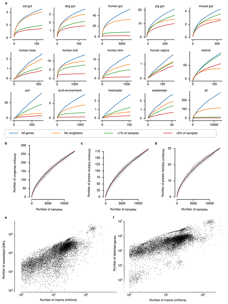
Extended Data Fig. 1. Gene accumulation curves.

(a) For most (but not all) habitats, unigenes with high prevalence (≥ 5%) have been well-captured, while rare unigenes continue to be found in each new sample. (b-d) New unigenes continue to be found in each sample. Each grey line represents a random permutation of the samples, while the solid black line shows the mean over these random permutations. The dotted red line is least-squares fit of Heap’s Law (N = k · sample^alpha). In all cases, the parameter fit indicates that the number of has not reached saturation. (e) The number of assembled/ detected genes per sample grows with sequencing depth without a plateau being reached. (f) Similarly, the number of detected ORFs per insert grows with sequencing depth.

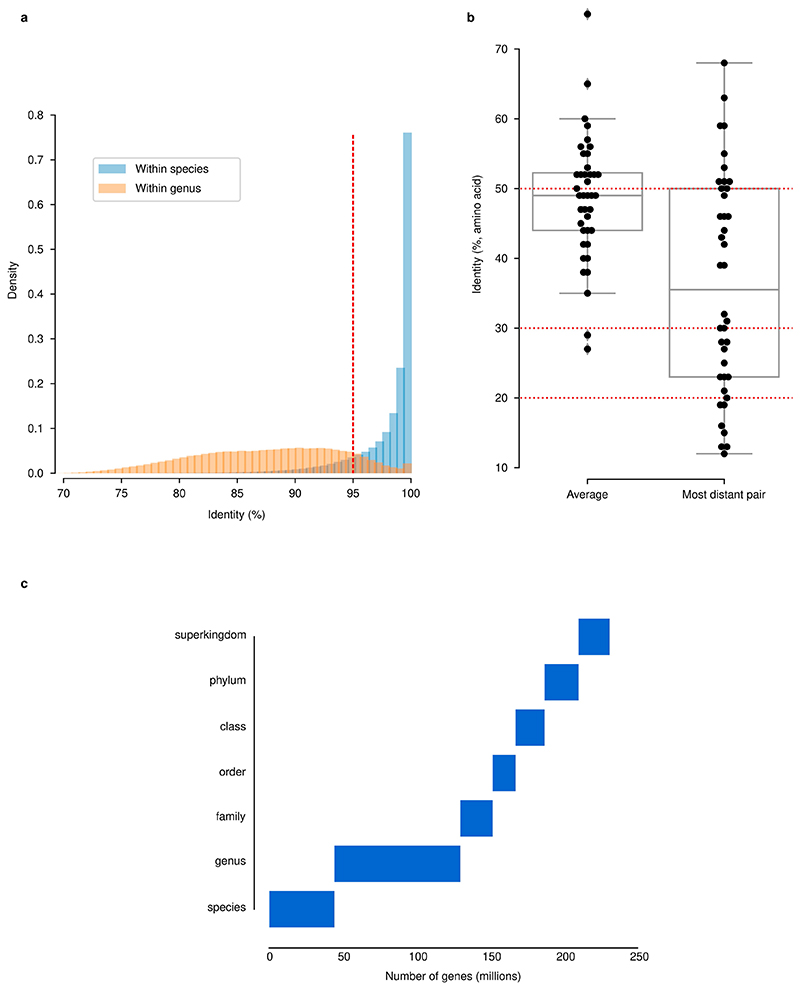
Extended Data Fig. 2. Identity thresholds and their relationship to taxonomy and function in the GMGCv1.

(a) A 95% nucleotide identity threshold is a proxy for species. Shown is nucleotide identity of closest gene homolog within the same species or within the same genus (excluding within-species comparisons). The threshold used in this work (95%) is marked with a dashed red line. (b) Within well-conserved, universal, 40 single-copy orthologues (see Methods), the average pairwise amino acid identity is 49%, albeit with a wide range (27-75%) when considering within-orthologue averages. In dashed red, the thresholds used for building protein families are highlighted. Boxplots display quartiles and ranges (see Methods). (c) Proportion of genes annotated at each taxonomic level.

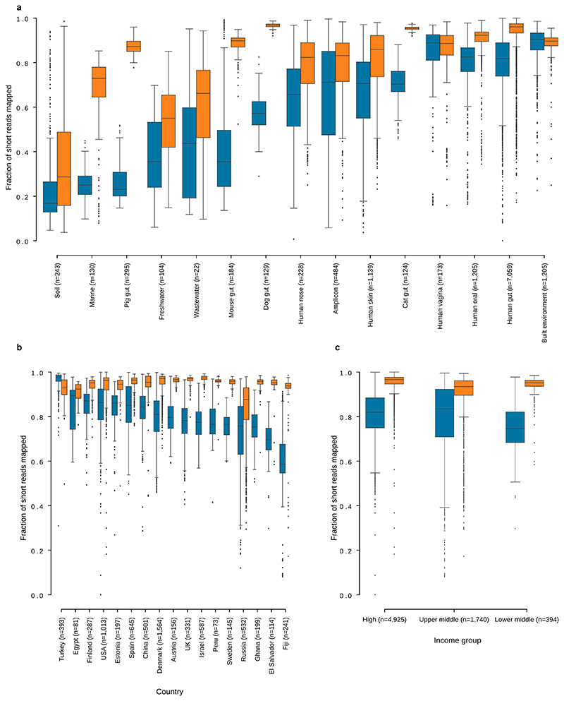
Extended Data Fig. 3. Short reads map to the GMGCv1 at higher rates (compared to a reference database of reference genomes).

(a) Mapping rates for short reads from metagenomes mapped against the GMGCv1 or the reference genomes in proGenomes2. (b) Fraction of short reads from human gut metagenomes mapping to a collection of sequenced genomes and the GMGCv1, per country, (c) Same data as (b), aggregated by the World Bank’s classification of countries into income groups. In all panels, boxplots show quartiles (including median) and range (except for outliers, see Methods). Blue boxes show mapping rates to proGenomes2, while orange boxes show mapping rates to GMGCv1.

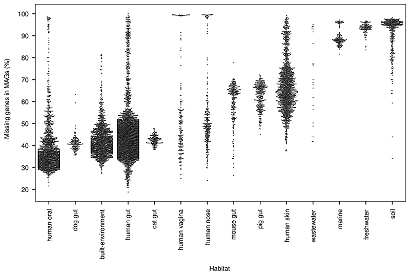
Extended Data Fig. 4. MAGs only capture a small fraction of all genes in a sample.

Fraction of undetected genes when mapping to only the genes captured by metagenome-assembled genomes (MAGs) across the habitats compared to mapping to the full GMGCv1.

Extended Data Fig. 5. Species and protein cluster sharing between habitats is similar to unigene sharing, but sharing of protein families is more extensive.

(a) The sharing of metagenomic species between habitats mimics unigene sharing. Width of each ribbons represents the number of MGSs shared between the habitats (the largest number shared is between the human and the pig gut, which share 166 MGSs out of 1,908 MGSs in the human gut and 898 in pig gut, respectively). (b) Species-level unigene sharing between habitats by fraction of the number of unigenes from each habitat (cf. Fig. 1b, which uses abundance weighting). (c) Sharing of protein clusters (90% amino acid identity clusters) between habitats, abundance-weighted. (d) Sharing of protein families between habitats, abundance-weighted. When considering coarser clusterings of sequences, gene sharing between habitats increases, yet we still observed higher rates of sharing between similar habitats and significant fractions of habitat-specific families (e.g., in the marine environment, 31.3% of the genes, by abundance, are in marine-specific protein families).

Extended Data Fig. 6. Antibiotic resistance and mobile genes are more likely to be multi-habitat genes, while most species are found in a single habitat.

(a) Fraction of unigenes within each habitat which are multi-habitat genes (for all unigenes, or when considering only mobile elements or antibiotic resistance genes). (b) A total of 7,443 MGSs were built, across all the habitats as species proxies to reliably assess their habitats. Each circle shows the number of metagenomic species for each habitat, x-axis represents the number of genes in the catalogue specific to each habitat, the y-axis represents the number of samples. Note that differing sampling depth and habitat-specific biodiversity impact those numbers.

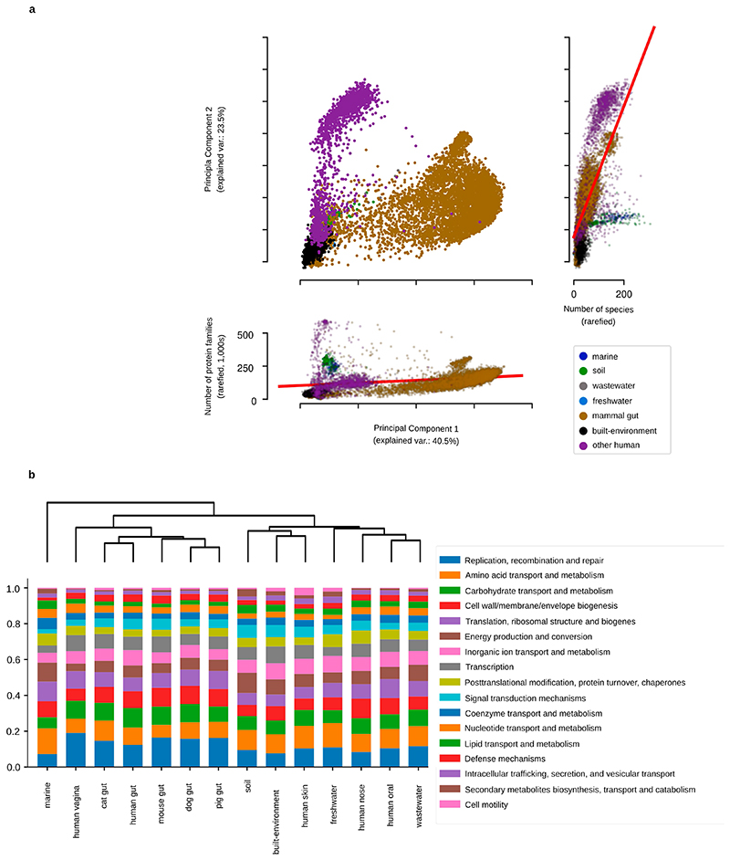
Extended Data Fig. 7. Determinants of functional community structure.

(a) principal coordinate analysis of all samples by protein family profile and the correlations with taxonomic and protein family richness (after rarefying to 1 million inserts to remove effects of sample depth). (b) Hierarchical clustering of the habitats using high-level functional profiles based.

Extended Data Fig. 8. Marine and soil richness patterns are a mixture of subpatterns.

Conspecific genes per species in marine (a) and (b) soil sub-habitats. The differences in the marine environment are particularly large when comparing the samples in the photic zones (the shallower, light-accessible, surface and deep-chlorophyll maximum samples) to the non-photic mesopelagic samples (deeper, beyond the reach of sunlight). The differences in the soil environment follow differences in acidity (with Podzol, Dystric Brunisol and Ultic soils being acidic, while Luvisols are usually neutral or alkaline) and differences in moisture (with Xeralfs being dry in the summer, while Glossudalfs are moist year round).

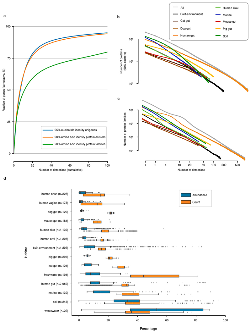
Extended Data Fig. 9. Most genes are detected only infrequently and rare genes are (on average) present at a lower abundance in metagenomes.

(a) Shown are the percentage of genes detected in at most 1,...,50 metagenomes (out of a total of 13,174). (b, c) Histograms of gene prevalence are roughly linear on a log-log scale, as predicted from neutral or nearly-neutral evolution models. Shown are histograms for 90% amino acid identity protein clusters (b) and 20% amino acid identity protein families (c), which behave similar to species-level unigenes (see Fig. 3). (d) Shown is the percentage of genes in each sample that is composed of rare genes (Count) and the total abundance represented by these (Abundance). Except for wastewater (likely due to under-sampling), rare genes represent a lower fraction of the abundance than of detection. Boxplots show quartiles (including median drawn as a line) and whiskers show the range of the data excluding outliers, which are shown as extra elements (see Methods).

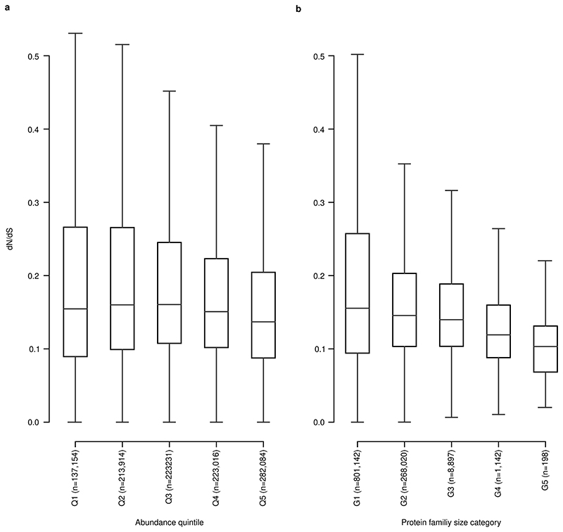
Extended Data Fig. 10. More abundant and larger protein families are under more intense selection.

(a) dN/dS within each protein family, with protein families split into 5 abundance quintiles, showing a downward trend with abundance (higher negative selection). (b) dN/dS within each gene size category, similarly showing a downward trend with size. Categories are defined by increasing size, with each bin representing the same number of unigenes. Boxplots show quartiles and ranges (see Methods).

Data Availability

All data analysed during the current study are publicly available. Supplementary Table 1 contains the accession numbers for all the metagenomes used. GMGCv1 is available for download at https://gmgc.embl.de. The full catalogue is available for download as are sub-catalogues specialized to individual habitats and the subset derived only from sequenced genomes (which can be further subset to obtain the pangenome of a species of interest). Both the full catalogue and a version containing only complete ORFs are available as they represent different tradeoffs: the complete catalogue achieves higher coverage, while the version with only complete ORFs may be more appropriate for analyses that require the whole gene. Similarly, protein families are available at different amino acid identity thresholds (see ‘Protein family cluster calculation’). In addition to being available for download, the catalogue can be queried with an amino acid sequence. We developed and use a novel k-mer based algorithm (see ‘k-mer based homology search’) to enable fast queries over the complete 303 million protein database and allow interactive use.

Code availability

The source code implementing the analyses in this manuscript is available on Github (https://github.com/luispedro/Coelho2021_GMGCv1) and is archived at Zenodo (https://doi.org/10.5281/zenodo.4769556).

References

- 1.Sunagawa S, et al. Structure and function of the global ocean microbiome. Science. 2015;348:1261359. doi: 10.1126/science.1261359. [DOI] [PubMed] [Google Scholar]
- 2.Zou Y, et al. 1,520 reference genomes from cultivated human gut bacteria enable functional microbiome analyses. Nat Biotechnol. 2019;37:179–185. doi: 10.1038/s41587-018-0008-8. [DOI] [PMC free article] [PubMed] [Google Scholar]
- 3.Mohammad BF, et al. Structure and function of the global topsoil microbiome. Nature. 2018;560:233–237. doi: 10.1038/s41586-018-0386-6. [DOI] [PubMed] [Google Scholar]
- 4.Qin J, et al. A human gut microbial gene catalogue established by metagenomic sequencing. Nature. 2010;464:59–65. doi: 10.1038/nature08821. [DOI] [PMC free article] [PubMed] [Google Scholar]
- 5.Xiao L, et al. A catalog of the mouse gut metagenome. Nat Biotechnol. 2015;33:1103–1108. doi: 10.1038/nbt.3353. [DOI] [PubMed] [Google Scholar]
- 6.Coelho LP, et al. Similarity of the dog and human gut microbiomes in gene content and response to diet. Microbiome. 2018;6:72. doi: 10.1186/s40168-018-0450-3. [DOI] [PMC free article] [PubMed] [Google Scholar]
- 7.Pasolli E, et al. Extensive unexplored human microbiome diversity revealed by over 150,000 genomes from metagenomes spanning age, geography, and lifestyle. Cell. 2019;176:649–662.:e20. doi: 10.1016/j.cell.2019.01.001. [DOI] [PMC free article] [PubMed] [Google Scholar]
- 8.Partridge SR, Kwong SM, Firth N, Jensen SO. Mobile genetic elements associated with antimicrobial resistance. Clin Microbiol Rev. 2018;31 doi: 10.1128/CMR.00088-17. [DOI] [PMC free article] [PubMed] [Google Scholar]
- 9.Mende DR, et al. ProGenomes2: An improved database for accurate and consistent habitat, taxonomic and functional annotations of prokaryotic genomes. Nucleic Acids Res. 2020;48:D621–D625. doi: 10.1093/nar/gkz1002. [DOI] [PMC free article] [PubMed] [Google Scholar]
- 10.Jain C, Rodriguez-R LM, Phillippy AM, Konstantinidis KT, Aluru S. High throughput ANI analysis of 90K prokaryotic genomes reveals clear species boundaries. Nat Commun. 2018;9:5114. doi: 10.1038/s41467-018-07641-9. [DOI] [PMC free article] [PubMed] [Google Scholar]
- 11.Steinegger M, Söding J. MMseqs2 enables sensitive protein sequence searching for the analysis of massive data sets. Nat Biotechnol. 2017;35:1026–1028. doi: 10.1038/nbt.3988. [DOI] [PubMed] [Google Scholar]
- 12.Daniel H, et al. RefSeq: an update on prokaryotic genome annotation and curation. Nuc Acids Res. 2018;46:D851–D860. doi: 10.1093/nar/gkx1068. [DOI] [PMC free article] [PubMed] [Google Scholar]
- 13.von Mering C, et al. Quantitative phylogenetic assessment of microbial communities in diverse environments. Science. 2007;315:1126–1130. doi: 10.1126/science.1133420. [DOI] [PubMed] [Google Scholar]
- 14.Richardson EJ, et al. Gene exchange drives the ecological success of a multi-host bacterial pathogen. Nat Ecol Evol. 2018;2:1468–1478. doi: 10.1038/s41559-018-0617-0. [DOI] [PMC free article] [PubMed] [Google Scholar]
- 15.Nielsen HB, et al. Identification and assembly of genomes and genetic elements in complex metagenomic samples without using reference genomes. Nat Biotechnol. 2014;32:822–828. doi: 10.1038/nbt.2939. [DOI] [PubMed] [Google Scholar]
- 16.Mende DR, Sunagawa S, Zeller G, Bork P. Accurate and universal delineation of prokaryotic species. Nat Methods. 2013;10:881–884. doi: 10.1038/nmeth.2575. [DOI] [PubMed] [Google Scholar]
- 17.Huerta-Cepas J, et al. Fast genome-wide functional annotation through orthology assignment by eggNOG-mapper. Mol Biol Evol. 2017;34:2115–2122. doi: 10.1093/molbev/msx148. [DOI] [PMC free article] [PubMed] [Google Scholar]
- 18.Louca S, et al. Function and functional redundancy in microbial systems. Nat Ecol Evol. 2018;2:936–943. doi: 10.1038/s41559-018-0519-1. [DOI] [PubMed] [Google Scholar]
- 19.Maistrenko OM, et al. Disentangling the impact of environmental and phylogenetic constraints on prokaryotic within-species diversity. ISME J. 2020;14:1247–1259. doi: 10.1038/s41396-020-0600-z. [DOI] [PMC free article] [PubMed] [Google Scholar]
- 20.Baumdicker F, Hess WR, Pfaffelhuber P. The diversity of a distributed genome in bacterial populations. Ann Appl Probab. 2010;20:1567–1606. [Google Scholar]
- 21.Sela I, Wolf YI, Koonin EV. Theory of prokaryotic genome evolution. Proc Natl Acad Sci USA. 2016;113:11399–11407. doi: 10.1073/pnas.1614083113. [DOI] [PMC free article] [PubMed] [Google Scholar]
- 22.Dandekar T, Snel B, Huynen M, Bork P. Conservation of gene order: a fingerprint of proteins that physically interact. Trends Biochem Sci. 1998;23:324–328. doi: 10.1016/s0968-0004(98)01274-2. [DOI] [PubMed] [Google Scholar]
- 23.Nei M, Suzuki Y, Nozawa M. The neutral theory of molecular evolution in the genomic era. Annu Rev Genomics Hum Genet. 2010;11:265–289. doi: 10.1146/annurev-genom-082908-150129. [DOI] [PubMed] [Google Scholar]
- 24.Iranzo J, Cuesta JA, Manrubia S, Katsnelson MI, Koonin EV. Disentangling the effects of selection and loss bias on gene dynamics. Proc Natl Acad Sci USA. 2017;114:E5616–E5624. doi: 10.1073/pnas.1704925114. [DOI] [PMC free article] [PubMed] [Google Scholar]
- 25.Wolf YI, Makarova KS, Lobkovsky AE, Koonin EV. Two fundamentally different classes of microbial genes. Nat Microbiol. 2016;2:16208. doi: 10.1038/nmicrobiol.2016.208. [DOI] [PubMed] [Google Scholar]
- 26.Rasko DA, et al. The pangenome structure of Escherichia coli: comparative genomic analysis of E. coli commensal and pathogenic isolates. J Bacteriol. 2008;190:6881–6893. doi: 10.1128/JB.00619-08. [DOI] [PMC free article] [PubMed] [Google Scholar]
- 27.Koskella B, Hall LJ, Metcalf CJE. The microbiome beyond the horizon of ecological and evolutionary theory. Nat Ecol Evol. 2017;1:1606–1615. doi: 10.1038/s41559-017-0340-2. [DOI] [PubMed] [Google Scholar]
- 28.Liu R, et al. Gut microbiome and serum metabolome alterations in obesity and after weight-loss intervention. Nat Med. 2017;23:859–868. doi: 10.1038/nm.4358. [DOI] [PubMed] [Google Scholar]
- 29.Metcalf JL, et al. Microbial community assembly and metabolic function during mammalian corpse decomposition. Science. 2015;351:158–162. doi: 10.1126/science.aad2646. [DOI] [PubMed] [Google Scholar]
- 30.Vincent C, et al. Bloom and bust: intestinal microbiota dynamics in response to hospital exposures and Clostridium difficile colonization or infection. Microbiome. 2016;4:12. doi: 10.1186/s40168-016-0156-3. [DOI] [PMC free article] [PubMed] [Google Scholar]
- 31.Zeller G, et al. Potential of fecal microbiota for early-stage detection of colorectal cancer. Mol Syst Biol. 2014;10:766. doi: 10.15252/msb.20145645. [DOI] [PMC free article] [PubMed] [Google Scholar]
- 32.Gibson MK, et al. Developmental dynamics of the preterm infant gut microbiota and antibiotic resistome. Nat Microbiol. 2016;1:16024. doi: 10.1038/nmicrobiol.2016.24. [DOI] [PMC free article] [PubMed] [Google Scholar]
- 33.Zhang X, et al. The oral and gut microbiomes are perturbed in rheumatoid arthritis and partly normalized after treatment. Nat Med. 2015;21:895–905. doi: 10.1038/nm.3914. [DOI] [PubMed] [Google Scholar]
- 34.Brito IL, et al. Mobile genes in the human microbiome are structured from global to individual scales. Nature. 2016;535:435–439. doi: 10.1038/nature18927. [DOI] [PMC free article] [PubMed] [Google Scholar]
- 35.Vatanen T, et al. Variation in microbiome LPS immunogenicity contributes to autoimmunity in humans. Cell. 2016;165:842–853. doi: 10.1016/j.cell.2016.04.007. [DOI] [PMC free article] [PubMed] [Google Scholar]
- 36.Turnbaugh PJ, et al. The human microbiome project. Nature. 2007;449:804–810. doi: 10.1038/nature06244. [DOI] [PMC free article] [PubMed] [Google Scholar]
- 37.Hannigan GD, et al. The human skin double-stranded DNA virome: topographical and temporal diversity, genetic enrichment, and dynamic associations with the host microbiome. MBio. 2015;6:e01578-15. doi: 10.1128/mBio.01578-15. [DOI] [PMC free article] [PubMed] [Google Scholar]
- 38.Taft DH, et al. Intestinal microbiota of preterm infants differ over time and between hospitals. Microbiome. 2014;2:36. doi: 10.1186/2049-2618-2-36. [DOI] [PMC free article] [PubMed] [Google Scholar]
- 39.Zeevi D, et al. Personalized nutrition by prediction of glycemic responses. Cell. 2015;163:1079–1094. doi: 10.1016/j.cell.2015.11.001. [DOI] [PubMed] [Google Scholar]
- 40.Wilhelm RC, et al. Biogeography and organic matter removal shape long-term effects of timber harvesting on forest soil microbial communities. ISME J. 2017;11:2552–2568. doi: 10.1038/ismej.2017.109. [DOI] [PMC free article] [PubMed] [Google Scholar]
- 41.Xie H, et al. Shotgun metagenomics of 250 adult twins reveals genetic and environmental impacts on the gut microbiome. Cell Syst. 2016;3:572–584.:e3. doi: 10.1016/j.cels.2016.10.004. [DOI] [PMC free article] [PubMed] [Google Scholar]
- 42.The MetaSUB International Consortium. The metagenomics and metadesign of the subways and urban biomes (metasub) international consortium inaugural meeting report. Microbiome. 2016;4:24. doi: 10.1186/s40168-016-0168-z. [DOI] [PMC free article] [PubMed] [Google Scholar]
- 43.Chatelier EL, et al. Richness of human gut microbiome correlates with metabolic markers. Nature. 2013;500:541–546. doi: 10.1038/nature12506. [DOI] [PubMed] [Google Scholar]
- 44.Li J, et al. Gut microbiota dysbiosis contributes to the development of hypertension. Microbiome. 2017;5 doi: 10.1186/s40168-016-0222-x. [DOI] [PMC free article] [PubMed] [Google Scholar]
- 45.Pehrsson EC, et al. Interconnected microbiomes and resistomes in low-income human habitats. Nature. 2016;533:212–216. doi: 10.1038/nature17672. [DOI] [PMC free article] [PubMed] [Google Scholar]
- 46.Li J, et al. An integrated catalog of reference genes in the human gut microbiome. Nat Biotechnol. 2014;32:834–841. doi: 10.1038/nbt.2942. [DOI] [PubMed] [Google Scholar]
- 47.Feng Q, et al. Gut microbiome development along the colorectal adenoma–carcinoma sequence. Nat Commun. 2015;6:6528. doi: 10.1038/ncomms7528. [DOI] [PubMed] [Google Scholar]
- 48.Gu Y, et al. Analyses of gut microbiota and plasma bile acids enable stratification of patients for antidiabetic treatment. Nat Commun. 2017;8:1785. doi: 10.1038/s41467-017-01682-2. [DOI] [PMC free article] [PubMed] [Google Scholar]
- 49.Karlsson FH, et al. Gut metagenome in european women with normal, impaired and diabetic glucose control. Nature. 2013;498:99–103. doi: 10.1038/nature12198. [DOI] [PubMed] [Google Scholar]
- 50.Yu J, et al. Metagenomic analysis of faecal microbiome as a tool towards targeted non-invasive biomarkers for colorectal cancer. Gut. 2017;66:70–78. doi: 10.1136/gutjnl-2015-309800. [DOI] [PubMed] [Google Scholar]
- 51.Youngster I, et al. Fecal microbiota transplant for relapsing clostridium difficile infection using a frozen inoculum from unrelated donors: a randomized, open-label, controlled pilot study. Clin Infect Dis. 2014;58:1515–1522. doi: 10.1093/cid/ciu135. [DOI] [PMC free article] [PubMed] [Google Scholar]
- 52.Guittar J, Shade A, Litchman E. Trait-based community assembly and succession of the infant gut microbiome. Nat Commun. 2019;10:512. doi: 10.1038/s41467-019-08377-w. [DOI] [PMC free article] [PubMed] [Google Scholar]
- 53.Vogtmann E, et al. Colorectal cancer and the human gut microbiome: reproducibility with whole-genome shotgun sequencing. PLoS ONE. 2016;11:e0155362. doi: 10.1371/journal.pone.0155362. [DOI] [PMC free article] [PubMed] [Google Scholar]
- 54.Chng KR, et al. Whole metagenome profiling reveals skin microbiome-dependent susceptibility to atopic dermatitis flare. Nat Microbiol. 2016;1:16106. doi: 10.1038/nmicrobiol.2016.106. [DOI] [PubMed] [Google Scholar]
- 55.Chu DM, et al. Maturation of the infant microbiome community structure and function across multiple body sites and in relation to mode of delivery. Nat Med. 2017;23:314–326. doi: 10.1038/nm.4272. [DOI] [PMC free article] [PubMed] [Google Scholar]
- 56.Van Rossum T, et al. Spatiotemporal dynamics of river viruses, bacteria and microeukaryotes. 2018 doi: 10.1101/259861. [DOI] [Google Scholar]
- 57.Feng Q, et al. Integrated metabolomics and metagenomics analysis of plasma and urine identified microbial metabolites associated with coronary heart disease. Sci Rep. 2016;6:22525. doi: 10.1038/srep22525. [DOI] [PMC free article] [PubMed] [Google Scholar]
- 58.Oh J, Byrd AL, Park M, Kong HH, Segre JA. Temporal stability of the human skin microbiome. Cell. 2016;165:854–866. doi: 10.1016/j.cell.2016.04.008. [DOI] [PMC free article] [PubMed] [Google Scholar]
- 59.Xiao L, et al. A reference gene catalogue of the pig gut microbiome. Nat Microbiol. 2016;1:16161. doi: 10.1038/nmicrobiol.2016.161. [DOI] [PubMed] [Google Scholar]
- 60.R Core Team. R: a language and environment for statistical computing. R Foundation for Statistical Computing; 2014. [Google Scholar]
- 61.Coelho LP, et al. NG-meta-profiler: Fast processing of metagenomes using ngless, a domain-specific language. Microbiome. 2019;7:84. doi: 10.1186/s40168-019-0684-8. [DOI] [PMC free article] [PubMed] [Google Scholar]
- 62.Li D, Liu C-M, Luo R, Sadakane K, Lam T-W. MEGAHIT: an ultra-fast single-node solution for large and complex metagenomics assembly via succinct De Bruijn graph. Bioinformatics. 2015;31:1674–1676. doi: 10.1093/bioinformatics/btv033. [DOI] [PubMed] [Google Scholar]
- 63.Besemer J, Borodovsky M. GeneMark: web software for gene finding in prokaryotes, eukaryotes and viruses. Nucleic Acids Res. 2005;33:W451–W454. doi: 10.1093/nar/gki487. [DOI] [PMC free article] [PubMed] [Google Scholar]
- 64.Coelho LP. Jug: Software for parallel reproducible computation in Python. J Open Res Softw. 2017;5:30. [Google Scholar]
- 65.Buchfink B, Xie C, Huson DH. Fast and sensitive protein alignment using diamond. Nat Methods. 2015;12:59–60. doi: 10.1038/nmeth.3176. [DOI] [PubMed] [Google Scholar]
- 66.Eberhardt RY, et al. AntiFam: A tool to help identify spurious ORFs in protein annotation. Database. 2012;2012:bas003. doi: 10.1093/database/bas003. [DOI] [PMC free article] [PubMed] [Google Scholar]
- 67.Kang D, et al. MetaBAT 2: An adaptive binning algorithm for robust and efficient genome reconstruction from metagenome assemblies. PeerJ. 2019;7:e7359. doi: 10.7717/peerj.7359. [DOI] [PMC free article] [PubMed] [Google Scholar]
- 68.Li H. Aligning sequence reads, clone sequences and assembly contigs with bwa-mem. 2013 Preprint at https://arxiv.org/abs/1303.3997. [Google Scholar]
- 69.Parks DH, Imelfort M, Skennerton CT, Hugenholtz P, Tyson GW. CheckM: assessing the quality of microbial genomes recovered from isolates, single cells, and metagenomes. Genome Res. 2015;25:1043–1055. doi: 10.1101/gr.186072.114. [DOI] [PMC free article] [PubMed] [Google Scholar]
- 70.Bowers RM, et al. Minimum information about a single amplified genome (MISAG) and a metagenome-assembled genome (MIMAG) of bacteria and archaea. Nat Biotechnol. 2017;35:725–731. doi: 10.1038/nbt.3893. [DOI] [PMC free article] [PubMed] [Google Scholar]
- 71.Zhou W, Gay N, Oh J. ReprDB and panDB: minimalist databases with maximal microbial representation. Microbiome. 2018;6:15. doi: 10.1186/s40168-018-0399-2. [DOI] [PMC free article] [PubMed] [Google Scholar]
- 72.Hingamp P, et al. Exploring nucleo-cytoplasmic large DNA viruses in tara oceans microbial metagenomes. ISME J. 2013;7:1678–1695. doi: 10.1038/ismej.2013.59. [DOI] [PMC free article] [PubMed] [Google Scholar]
- 73.Seemann T. Prokka: rapid prokaryotic genome annotation. Bioinformatics. 2014;30:2068–2069. doi: 10.1093/bioinformatics/btu153. [DOI] [PubMed] [Google Scholar]
- 74.Huerta-Cepas J, et al. eggNOG 5.0: A hierarchical, functionally and phylogenetically annotated orthology resource based on 5090 organisms and 2502 viruses. Nucleic Acids Res. 2019;47:D309–D314. doi: 10.1093/nar/gky1085. [DOI] [PMC free article] [PubMed] [Google Scholar]
- 75.Eddy SR. Accelerated profile HMM searches. PLoS Comput Biol. 2011;7:e1002195. doi: 10.1371/journal.pcbi.1002195. [DOI] [PMC free article] [PubMed] [Google Scholar]
- 76.Smyshlyaev G, Barabas O, Bateman A. Sequence analysis allows functional annotation of tyrosine recombinases in prokaryotic genomes. Mol Syst Biol. 2021;17:e9880. doi: 10.15252/msb.20209880. [DOI] [PMC free article] [PubMed] [Google Scholar]
- 77.Jia B, et al. CARD 2017: Expansion and model-centric curation of the comprehensive antibiotic resistance database. Nucleic Acids Res. 2017;45:D566–D573. doi: 10.1093/nar/gkw1004. [DOI] [PMC free article] [PubMed] [Google Scholar]
- 78.Gibson MK, Forsberg KJ, Dantas G. Improved annotation of antibiotic resistance determinants reveals microbial resistomes cluster by ecology. ISME J. 2015;9:207–216. doi: 10.1038/ismej.2014.106. [DOI] [PMC free article] [PubMed] [Google Scholar]
- 79.Li T, Fan K, Wang J, Wang W. Reduction of protein sequence complexity by residue grouping. Protein Eng. 2003;16:323–330. doi: 10.1093/protein/gzg044. [DOI] [PubMed] [Google Scholar]
- 80.Zhao M, Lee W-P, Garrison EP, Marth GT. SSW library: an SIMD Smith–Waterman C/C++ library for use in genomic applications. PLoS ONE. 2013;8:e82138. doi: 10.1371/journal.pone.0082138. [DOI] [PMC free article] [PubMed] [Google Scholar]
- 81.Li H. Minimap2: Pairwise alignment for nucleotide sequences. Bioinformatics. 2017;34:3094–3100. doi: 10.1093/bioinformatics/bty191. [DOI] [PMC free article] [PubMed] [Google Scholar]
- 82.Salter A, et al. Microbial abundance, activity and population genomic profiling with mOTUs2. Nat Commun. 2019;10:1014. doi: 10.1038/s41467-019-08844-4. [DOI] [PMC free article] [PubMed] [Google Scholar]
- 83.Salter SJ, et al. Reagent and laboratory contamination can critically impact sequence-based microbiome analyses. BMC Biol. 2014;12:87. doi: 10.1186/s12915-014-0087-z. [DOI] [PMC free article] [PubMed] [Google Scholar]
- 84.Kumar R, Acharya V, Singh D, Kumar S. Strategies for high-altitude adaptation revealed from high-quality draft genome of non-violacein producing Janthinobacterium lividum ERGS5:01. Stand Genomic Sci. 2018;13:11. doi: 10.1186/s40793-018-0313-3. [DOI] [PMC free article] [PubMed] [Google Scholar]
- 85.Patijanasoontorn B, et al. Hospital acquired Janthinobacterium lividum septicemia in srinagarind hospital. J Med Assoc Thai. 1992;75(Suppl 2):6–10. [PubMed] [Google Scholar]
- 86.Harris CR, et al. Array programming with NumPy. Nature. 2020;585:357–362. doi: 10.1038/s41586-020-2649-2. [DOI] [PMC free article] [PubMed] [Google Scholar]
- 87.Virtanen P, et al. SciPy 1.0: Fundamental algorithms for scientific computing in Python. Nat Methods. 2020;17:261–272. doi: 10.1038/s41592-019-0686-2. [DOI] [PMC free article] [PubMed] [Google Scholar]
- 88.Pedregosa F, et al. Scikit-learn: machine learning in Python. J Mach Learn Res. 2011;12:2825–2830. [Google Scholar]
- 89.Collins RE, Higgs PG. Testing the infinitely many genes model for the evolution of the bacterial core genome and pangenome. Mol Biol Evol. 2012;29:3413–3425. doi: 10.1093/molbev/mss163. [DOI] [PubMed] [Google Scholar]
- 90.Sievers F, et al. Fast, scalable generation of high-quality protein multiple sequence alignments using clustal omega. Mol Syst Biol. 2011;7:539. doi: 10.1038/msb.2011.75. [DOI] [PMC free article] [PubMed] [Google Scholar]
- 91.Price MN, Dehal PS, Arkin AP. FastTree 2—approximately maximum-likelihood trees for large alignments. PLoS ONE. 2010;5:e9490. doi: 10.1371/journal.pone.0009490. [DOI] [PMC free article] [PubMed] [Google Scholar]
- 92.Huerta-Cepas J, Serra F, Bork P. ETE 3: reconstruction, analysis, and visualization of phylogenomic data. Mol Biol Evol. 2016;33:1635–1638. doi: 10.1093/molbev/msw046. [DOI] [PMC free article] [PubMed] [Google Scholar]
- 93.Edgar RC. MUSCLE: multiple sequence alignment with high accuracy and high throughput. Nucleic Acids Res. 2004;32:1792–1797. doi: 10.1093/nar/gkh340. [DOI] [PMC free article] [PubMed] [Google Scholar]
- 94.Suyama M, Torrents D, Bork P. PAL2NAL: robust conversion of protein sequence alignments into the corresponding codon alignments. Nucleic Acids Res. 2006;34:W609-12. doi: 10.1093/nar/gkl315. [DOI] [PMC free article] [PubMed] [Google Scholar]
- 95.Murrell B, et al. FUBAR: a fast, unconstrained Bayesian approximation for inferring selection. Mol Biol Evol. 2013;30:1196–1205. doi: 10.1093/molbev/mst030. [DOI] [PMC free article] [PubMed] [Google Scholar]
- 96.Smith MD, et al. Less is more: an adaptive branch-site random effects model for efficient detection of episodic diversifying selection. Mol Biol Evol. 2015;32:1342–1353. doi: 10.1093/molbev/msv022. [DOI] [PMC free article] [PubMed] [Google Scholar]
- 97.Washietl S, et al. RNAcode: robust discrimination of coding and noncoding regions in comparative sequence data. RNA. 2011;17:578–594. doi: 10.1261/rna.2536111. [DOI] [PMC free article] [PubMed] [Google Scholar]
Associated Data
This section collects any data citations, data availability statements, or supplementary materials included in this article.
Supplementary Materials
Data Availability Statement