Estimation of dynamic sparse connectivity patterns from resting state fMRI

Abstract

Functional connectivity (FC) estimated from functional magnetic resonance imaging (fMRI) time series, especially during resting state periods, provides a powerful tool to assess human brain functional architecture in health, disease, and developmental states. Recently, the focus of connectivity analysis has shifted towards the subnetworks of the brain, which reveals co-activating patterns over time. Most prior works produced a dense set of high-dimensional vectors, which are hard to interpret. In addition, their estimations to a large extent were based on an implicit assumption of spatial and temporal stationarity throughout the fMRI scanning session. In this study, we propose an approach called dynamic sparse connectivity patterns (dSCPs), which takes advantage of both matrix factorization and time-varying fMRI time series to improve the estimation power of FC. The feasibility of analyzing dynamic FC with our model is first validated through simulated experiments. Then, we use our framework to measure the difference between young adults and children with real fMRI dataset from the Philadelphia Neurodevelopmental Cohort (PNC). The results from the PNC dataset showed significant FC differences between young adults and children in 4 different states. For instance, young adults had reduced connectivity between the default mode network and other subnetworks, as well as hyperconnectivity within the visual system in states 1 and 3, and hypoconnectivity in state 2. Meanwhile, they exhibited temporal correlation patterns that changed over time within functional subnetworks. In addition, the dSCPs model indicated that older people tend to spend more time within a relatively connected FC pattern. Overall, the proposed method provides a valid means to assess dynamic FC, which could facilitate the study of brain networks.

I. Introduction

The human brain is a complex system that contains functional entities that interact with each other to respond to both internal and external stimuli. Connectivity within the brain may be altered by mental disorders or during developmental stages. Du et al. found brain FC differences among patients, diagnosed with bipolar disorder with psychosis (BPP), schizoaffective disorder (SAD), and schizophrenia (SZ) in multiple functional networks [1], [2]. Khadka et al. identified significant alterations in 7 functional networks for SZ, BPP and their 1st degree relatives [3]. Prior research has shown that connections among intrinsic connectivity networks (ICNs) vary with increasing age [4], [5]. Thus, an accurate characterization of the brain’s functional connectivity benefits from understanding both normal brain development and abnormal brain function in patients.

Recently, the focus of connectivity analysis has shifted from merely localizing activations and deactivations towards brain functional network identification, which reveals co-activating patterns over time [6]. Various computational approaches have been proposed to identify such sub-networks. One such method is seed-based correlation analysis, which relies on statistical hypothesis testing to reveal brain connectivity (e.g.[7]). Seed-based methods are sensitive to the selection of the seed regions [8]. The choice of seed may bias connectivity findings towards specific, smaller or overlapping sub-systems, instead of large, distinct networks [9]. Conversely, brain connectivity maps can be based on data-driven approaches. Graph partitioning methodologies such as InfoMap assume that any region of the brain can belong to only one brain network [10], [11]. Matrix factorization approaches, including Independent Component Analysis (ICA), Non-negative Matrix Factorization (NMF), Principle Component Analysis (PCA), are also widely used[12], [13], [14]. ICA is increasingly utilized as a tool for evaluating the hidden spatio/temporal structure from fMRI blood-oxygenation-level dependent (BOLD) time series [12]. In brief, NMF sometimes can be viewed as a positively-constrained version of ICA [13]. PCA is combined with ICA in some cases to extract ICNs from fMRI data [6], [14]. Recently, sparse representation and dictionary learning methods have attracted increasing attention in fMRI data analysis. Many novel frameworks have been proposed to develop sparse representation of fMRI signals [15], [16], [17], [18]. For example, Eavani et al. proposed a sparse connectivity patterns (SCPs) extraction method using spatial sparsity to achieve network identification [19]. SCPs are extracted from each subject’s pairwise correlation matrices. A similar idea which represents covariance matrices with low dimensional subspace has also been used in tensor decomposition works [20], [21], [22], [23]. Further details about their formulation and estimation are provided in the next section. Inspired by this work, we developed a method relying on a generalized fused Lasso penalty to analyze similarities and differences in functional connectivity between children and young adults [24].

For the approaches discussed above, functional connectivity estimation is largely based on the implicit assumption that coactivation among brain regions remains stationary throughout the fMRI scanning session [6]. The methods exploiting this assumption are normally called static FC approaches. Static FC techniques can provide key information regarding the topological organization of functional brain networks. However, when static FC approaches are utilized for rsfMRI, the stationary hypothesis may not hold, as spontaneous fluctuations of activity and connectivity are potentially prominent in the resting state due to unconstrained mental activity. Recently, advances in dynamic FC have been shown to be advantageous in this regard [25], [26]. Dynamic FC studies have identified reoccurring patterns of brain FC with improved reproducibility across individuals, which have the potential for illuminating differences in the dynamic connectivity of various mental illnesses [6], [26], [27], [28], [29]. Dynamic FC methods can also help us quantify the interplay within and between functional brain networks over short time scales. In sum, dynamic approaches overcome the limitations of the static model and capture the time-varying nature of brain networks. Thus, the motivation of this paper is to introduce a new framework for the estimation of dynamic sparse connectivity patterns (dSCPs). In the work of Eavani et al. [19] as well as ours [24], a global set of SCPs for the entire fMRI scanning session is extracted. Compared to these studies, we exploit the sliding window technique to capture dynamic connectivity among ICNs in the current study. In addition, with sparsity enforcement, the new model reduces the high dimensionality of the connectivity network to a small set of strongly correlated regions, leading to more interpretable results.

In the following sections, we first introduce the estimating SCPs, and then extend it to estimate dynamic SCPs for time series data in Section 2. We then validate our dynamic SCP estimation framework using both simulated and real datasets in Section 3. In particular, we investigate the use of dSCPs on a large fMRI dataset (PNC) to analyze the differences of FC between young adults and children [30]. Some discussions and concluding remarks are given in Sections 4 and 5.

II. Methods

A. Identification of Dynamic Sparse Connectivity Patterns

Sparse connectivity patterns (SCPs) were first defined by Eavani et al. to study brain networks [19]. Let us assume that we have $n\in \mathbb{N}$ subjects, n_t time points and p ROIs $\left(n_t,p\in \mathbb{N}\right)$ from a BOLD time series of each subject. The input to the SCPs estimation model is a p × p correlation matrix $C_i\left(C_i\in {ℝ}^{p\times p}\right)$, one for each subject i, i ∈ 1, 2, …, n. Here, C_i(b₁, b₂) is the Pearson correlation between ROIs b₁ and b₂ across the entire BOLD time series. We would like to approximate each matrix C_i by $d\in \mathbb{N}\left(d\le p\right)$ SCPs by solving the following problem:

$$\begin{gathered} \underset{\text{x}\in {ℝ}^{p\times d},\text{W}}{\min }\frac{1}{2}\sum _{i=1}^n{\Vert C_i-\text{x}{W}_i{\text{x}}^T\Vert }_F^2+\lambda {\Vert \text{x}\Vert }_1 \\ \text{subject}\hspace{0.17em}\text{to}{\Vert x_j\Vert }_{\infty }=1,j\in 1,2,\dots ,d \\ \hspace{0.17em}\hspace{1em}\hspace{1em}\hspace{1em}{W}_i\ge 0,{\forall }_i\in 1,2,\dots n \end{gathered}$$ (1)

where λ is a non-negative model parameter, || · ||_F denotes the Frobenius norm, each column of $\text{x}=\left[x_1,x_2,\dots ,x_d\right]\in {ℝ}^{p\times d}$ defines a SCP representing a set of co-activated regions, $W_i\in {ℝ}^{d\times d}$, ∀_i ∈ 1, 2, …, n is a diagonal matrix and W = {W₁, W₂, …, W_n}. Note that W_i ≥ 0 means that elements of each matrix W_i are assumed to be positive to maintain positive semidefinite and the constraint on each SCP x_j with infinity norm is used to avoid any scaling ambiguity [19]. The positive coefficients within each diagonal matrix W_i, provide ”subject-specific” maps, expressing how much a given SCP is articulated in the i^th subject’s correlation matrix C_i. If |x_i(k)| > 0, k = 1, 2 … d, node k belongs to the subnetwork Otherwise it does not. Note that if two nodes in x_i have the same sign, then they are positively correlated and vice versa. Such an approach reduces the high dimensionality of the correlation network by extracting a small set of strongly correlated components.

The model described in Eq.1 uses the full time series to compute the correlation matrix C_i. It makes the implicit assumption that co-activation between ROIs is constant over the entire scanning session. However, this assumption might be unreasonable for fMRI due to spontaneous fluctuations. Many related studies have demonstrated that meaningful information for functional brain networks can be extracted by taking into account the presence of temporal variability [6], [25], [26], [28], [29], [31]. To this end, we extend the model from Eq.1 using a sliding window approach along with time series. In this way, we can improve the estimate of functional connectivity changes over time.

Now, let us assume that $n_w\in \mathbb{N}$ correlation matrices are extracted using the sliding window technique [6] for each subject (we use a tapered window, which is created by convolving a rectangle with a Gaussian window and sliding in a step of 1 TR). We denote $C_{i,w}\in {ℝ}^{p\times p}$ the w^th correlation matrix for the i^th subject (w ∈ [1, 2, …, n_w]) and C_i,w(b₁, b₂) is the temporal Pearson correlation value between ROIs b₁ and b₂ for the w^th time window. Then, the model described in Eq.1 can be extended and the dynamic model is defined by the following equation:

$$\begin{gathered} \underset{\text{x}\in {ℝ}^{p\times d},\text{W}}{\min }\frac{1}{2}\sum _{i=1}^n\sum _{w=1}^{n_w}{\Vert C_{i,w}-\text{x}{W}_{i,w}{\text{x}}^T\Vert }_F^2+\lambda {\Vert \text{x}\Vert }_1 \\ \text{subject}\hspace{0.17em}\text{to}{\Vert x_j\Vert }_{\infty }=1,j=1,2,\dots d \\ \hspace{1em}\hspace{1em}\hspace{1em}{W}_{i,w}\ge 0,{\forall }_i=1,2,\dots ,n,w=1,2,\dots ,n_w \end{gathered}$$ (2)

where $W_{i,w}\in {ℝ}^{d\times d}$ is the subject-specific weighted matrix for the w^th window, and W = {W₁,₁, …, W_1,nw , …, W_n,1, …, W_n,nw } is the concatenation of each W_i,w for all subjects. The main difference between Eq.1 and Eq.2 lies in these subject-specific weighted maps in the following way: In Eq.1, only a single weight value is calculated for each subject and each SCP; in Eq.2, we have a set of n_w weight values for each subject and the corresponding SCP, which allows us to estimate time-varying connectivity. An illustration of the difference between these two approaches can be seen in Fig.1.

Fig. 1.

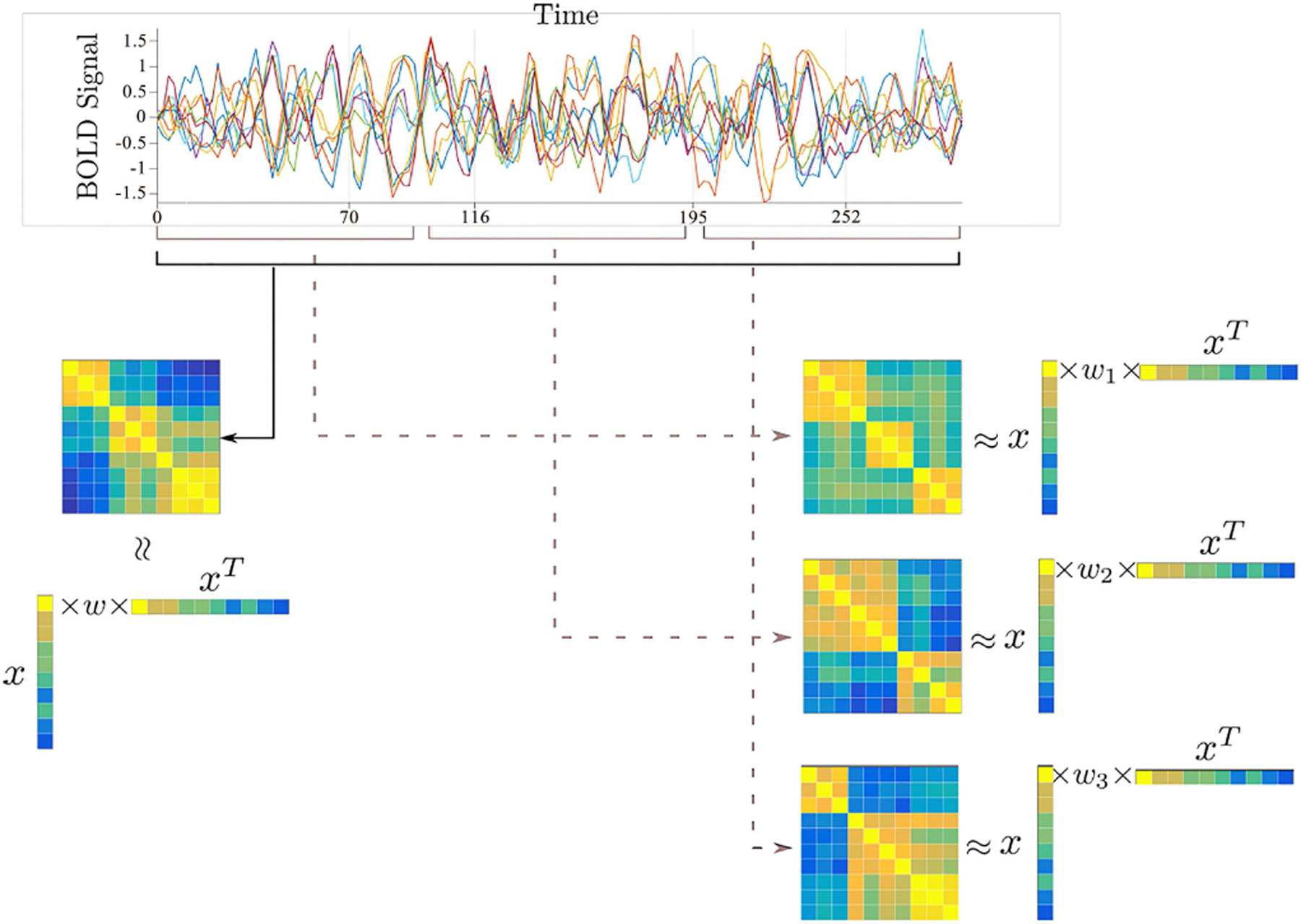
An illustration of the proposed formulation (right) versus original approach of Eavani et al. (left). The components of vectors x representing a set of subnetworks (SCPs) are extracted using Pearson correlation matrices. For each subject, only one weighted matrix is extracted in the model described by Eq.1. In our formulation defined by Eq.2, we now have a set of coefficients W_i,w, i = 1, 2, …, n, w = 1, 2, …, n_w for each subject, which leads to a richer description compared with the single coefficient W_i associated to x in the static model.

B. Optimization

In order to solve our proposed formulation defined by Eq.2, we can rely on the alternating direction method of multipliers (ADMM) [32]. The model defined in Eq.2 requires the minimization of a parameter that is the sum of n × n_w functions, with an additional sparse constraint on the solution x. Although these different parts do not split, due to the fact that x is shared across all the subjects and windows, we can still tackle it as a global consensus problem [32]. Consider the following general formulation:

$$\begin{gathered} \underset{x,z}{\min }\sum _{j=1}^{n}f\left(x_j\right)+g\left(z\right) \\ \text{subject}\hspace{0.17em}\text{to}\hspace{0.17em}{x}_j-z=0,j=1,2,\dots d \end{gathered}$$ (3)

where $d\in \mathbb{N}\left(d\le p\right)$ and x₁, x₂, …, x_d, $z\in {ℝ}^p$. Such a formulation considers d independent problems under the constraint that all local variables x_j should agree. By exploiting the function g, further constraints on each local variable can be added (for example, we can have g(x) := ||x||₁ ). Thus, we can handle the window problem in Eq.2 using the rearrangement from Eq.3 through the following notations:

$$\begin{gathered} f\left(x_j\right)=\sum _{i=1}^n\sum _{w=1}^{n_w}{\Vert C_{i,w}-x_j\left(W_{i,w}\right)x_j^T\Vert }_F^2 \\ \hspace{1em}\hspace{1em}\hspace{1em}\hspace{1em}\hspace{1em}g\left(z\right)=\lambda {\Vert z\Vert }_1 \end{gathered}$$ (4)

where i ∈ [1, 2, …, n] and w ∈ [1, 2, …, n_w]. The main advantage of ADMM is that by breaking down the original problem into a sequence of independent sub-problems, the associated minimization becomes much easier. The general minimization algorithm is detailed in Algorithm 1.

In our case, the starting point $x_j^0$ is initialized by calculating the 1st (the largest absolute magnitude) eigenvalue of correlation matrix C_j, and z⁰, $u_j^0$ are initialized at random. The

$$\underset{\_}{\begin{array}{l}\overline{\underset{\_}{\mathbf{\text{Algorithm}}\hspace{0.17em}\mathbf{1}\hspace{0.17em}\text{General}\hspace{0.17em}\text{ADMM}\hspace{0.17em}\text{minmization}\hspace{0.17em}\text{algorithm}}}\\ \hspace{0.17em}\hspace{0.17em}1:\hspace{0.17em}\text{Initialize}\hspace{0.17em}{x}_1^0,x_2^0,\dots ,x_d^0;u_1^0,u_2^0,\dots u_d^0;z^0\in {ℝ}^p\\ \hspace{0.17em}\hspace{0.17em}2:\text{Input}\hspace{0.17em}\text{regularization}\hspace{0.17em}\text{parameter}\hspace{0.17em}\rho \in ℝ\\ \hspace{0.17em}\hspace{0.17em}3:\mathbf{\text{for}}\hspace{0.17em}k=0\hspace{0.17em}\text{to}\hspace{0.17em}\text{Convergence}\hspace{0.17em}\mathbf{\text{do}}\\ \hspace{0.17em}\hspace{0.17em}4:\hspace{0.17em}\hspace{0.17em}\hspace{0.17em}{x}^{k+1}:=\arg \hspace{0.17em}{\min }_{xj}\left(f_j\left(x_j\right)+\frac{\rho }{2}{\Vert x_j-z^k+u_j^k\Vert }_2^2\right)\\ \hspace{0.17em}\hspace{0.17em}5:\hspace{0.17em}\hspace{0.17em}\hspace{0.17em}{z}^{k+1}:=\arg \hspace{0.17em}{\min }_z\left(g\left(z\right)+\frac{n\rho }{2}{\Vert z-{\overline{x}}_j^k-{\overline{u}}_j^k\Vert }_2^2\right)\\ \hspace{0.17em}\hspace{0.17em}6:\hspace{0.17em}\hspace{0.17em}\hspace{0.17em}{u}_j^{k+1}:=u_j^k+x_j^k-z^{k+1}\\ \hspace{0.17em}\hspace{0.17em}7:\mathbf{\text{end}}\hspace{0.17em}\mathbf{\text{for}}\end{array}}$$

x-update in Algorithm 1, line 4, is solved through gradient descent. The z-update in line 5, is achieved using the soft-thresholding method described in [33]. The estimation of SCPs takes place sequentially; that is, one after the other. After extracting the first SCP x₁ and its corresponding weighted maps $W_{i,w}^1,\forall \left(i,w\right)\in \left[1,n\right]\times \left[1,n_w\right]$, we can subtract the contribution of x₁ from each matrix C_i,w and define new matrices as:

$${\tilde{C}}_{i,w}=C_{i,w}-x_1\left(W_{i,w}^1\right){\left(x_1\right)}^T$$ (5)

The estimation of the second SCP can be performed as the calculation of all SCPs on the updated matrices ${\tilde{C}}_{i,w}^1$, $\forall \left(i,w\right)\in \left[1,n\right]\times \left[1.n_w\right]$. In such a way, we can calculate each SCP one by one, which simplifies the overall estimation. The estimation algorithm for dynamic SCPs can be obtained as detailed in Algorithm 2.

$$\underset{\_}{\begin{array}{l}\overline{\underset{\_}{\mathbf{\text{Algorithm}}\hspace{0.17em}\mathbf{2}\hspace{0.17em}\text{Dynamic}\hspace{0.17em}\text{SCPs}\hspace{0.17em}\text{estimation}\hspace{0.17em}\text{algorithm}}}\\ \hspace{0.17em}\hspace{0.17em}1:\hspace{0.17em}\text{Input}\hspace{0.17em}\text{parameter}\hspace{0.17em}l\\ \hspace{0.17em}\hspace{0.17em}2:\text{Compute}\hspace{0.17em}\text{correlation}\hspace{0.17em}\text{matrices}\hspace{0.17em}{C}_{i,w},\\ \hspace{0.17em}\hspace{0.17em}\hspace{0.17em}\hspace{0.17em}\hspace{0.17em}i=1,2,\dots ,n,w=1,2,\dots ,n_w\\ \hspace{0.17em}\hspace{0.17em}3:\text{Input}\hspace{0.17em}\text{parameter}\hspace{0.17em}\lambda ,d\\ \hspace{0.17em}\hspace{0.17em}4:\mathbf{\text{for}}\hspace{0.17em}r=1\hspace{0.17em}\text{to}\hspace{0.17em}d\hspace{0.17em}\mathbf{\text{do}}\\ \hspace{0.17em}\hspace{0.17em}5:\hspace{0.17em}\hspace{0.17em}\hspace{0.17em}\mathbf{\text{if}}\hspace{0.17em}r\ge 2\hspace{0.17em}\mathbf{\text{then}}\\ \hspace{0.17em}\hspace{0.17em}6:\hspace{0.17em}\hspace{0.17em}\hspace{0.17em}\hspace{0.17em}\hspace{0.17em}\text{Compute}\hspace{0.17em}\text{weights}\hspace{0.17em}\hspace{0.17em}\text{matrices}\hspace{0.17em}\hspace{0.17em}{W}_{i,w}^{1:r-1},\\ \hspace{0.17em}\hspace{0.17em}\hspace{0.17em}\hspace{0.17em}\hspace{0.17em}\hspace{0.17em}\hspace{0.17em}\hspace{0.17em}\hspace{0.17em}\hspace{0.17em}i=1,2\dots ,n\\ \hspace{0.17em}\hspace{0.17em}7:\hspace{0.17em}\hspace{0.17em}\hspace{0.17em}\hspace{0.17em}\hspace{0.17em}{\tilde{C}}_{i,w}:=C_{i,w}-x_{1:r-1}\left(W_{i,w}^{1:r-1}\right){\left(x_{1:r-1}\right)}^T\\ \hspace{0.17em}\hspace{0.17em}8:\hspace{0.17em}\hspace{0.17em}\hspace{0.17em}\mathbf{\text{else}}\\ \hspace{0.17em}\hspace{0.17em}9:\hspace{0.17em}\hspace{0.17em}\hspace{0.17em}\hspace{0.17em}\hspace{0.17em}{\tilde{C}}_{i,w}:=C_{i,w}\\ \hspace{0.17em}\hspace{0.17em}10:\hspace{0.17em}\hspace{0.17em}\mathbf{\text{end}}\hspace{0.17em}\mathbf{\text{if}}\\ \hspace{0.17em}\hspace{0.17em}11:\hspace{0.17em}\hspace{0.17em}\text{Estimate}\hspace{0.17em}{x}_r\hspace{0.17em}\text{using}\hspace{0.17em}{\tilde{C}}_{i,w}\hspace{0.17em}\text{and}\hspace{0.17em}\text{ADMM}\hspace{0.17em}\text{algorithm}\hspace{0.17em}1\\ \hspace{0.17em}\hspace{0.17em}12:\hspace{0.17em}\hspace{0.17em}\text{Normalize}\hspace{0.17em}{x}_r\hspace{0.17em}\text{such}\hspace{0.17em}\text{that}\hspace{0.17em}{\max }_i\left|x_r\left(i\right)\right|=1\\ \hspace{0.17em}\hspace{0.17em}13:\mathbf{\text{end}}\hspace{0.17em}\mathbf{\text{for}}\\ \hspace{0.17em}\hspace{0.17em}14:\text{Compute}\hspace{0.17em}\text{weight}\hspace{0.17em}\text{matrices}\hspace{0.17em}{W}_{i,w}^{1:r-1},\\ \hspace{0.17em}\hspace{0.17em}\hspace{0.17em}\hspace{0.17em}\hspace{0.17em}\hspace{0.17em}\hspace{0.17em}i=1,2\dots ,n\hspace{0.17em}\text{according}\hspace{0.17em}\text{to}\hspace{0.17em}\text{extracted}\hspace{0.17em}{x}_r\end{array}}$$

C. Tuning parameter selection

Finding optimal parameters is critical for the estimation of the proposed model. The dynamic SCPs estimation model defined in Eq.2 involves the use of three key parameters: the length of the sliding window l, the number of SCPs d, and the sparsity level of each SCP λ.

Typical window sizes range between 30 and 60 seconds [6], [34], [35], [36]. Note that for the sliding window selection, the smaller the number of time points within a window, the greater the chance of having inaccuracy and inducing spurious variability [34], [37]. As the regularization term λ controls the sparsity level of extracted SCPs, the larger the λ value is, the sparser the estimated SCPs are. In this work, we rely on the reconstruction error to estimate the optimal values for parameters l and λ. Both grid search and 5-fold cross-validation for parameters l and λ are performed, and the point corresponding to the lowest error is chosen to be the optimal one [19]. The reconstruction error is evaluated on the test set [19], defined as follows:

$$Test\hspace{0.17em}error=\frac{{\sum }_{i=1}^n{\sum }_{w=1}^{n_w}{\Vert C_{i,w}^{test}-{\text{x}}^{train}{W}_{i,w}^{test}{\left({\text{x}}^{train}\right)}^T\Vert }_F^2}{{\sum }_{i=1}^n{\sum }_{w=1}^{n_w}{\Vert C_{i,w}^{test}-{\overline{C}}_w^{test}\Vert }_F^2}$$ (6)

where superscripts test and train indicate the corresponding terms and are calculated from test and training sets, respectively. The component ${\overline{C}}_w^{test}$ is the subject-averaged correlation matrix for each window of the test dataset.

As the number of the SCPs d increases, the reconstruction error should be reduced. However, if d is beyond a certain number, the SCPs estimated by the algorithm could represent erroneous variations. Thus, it is difficult to optimize d according to the reconstruction error after parameters λ and l have been estimated. Here, we improve our accuracy to evaluate the optimal value of d through the use of classification. We use Support Vector Machine (SVM, referring to [38]) as the classifier and dynamic weighted matrices as the features to do the classification. We separate young adults and children in our real fMRI dataset, and divide the datasets into a training set (80%) and a testing set (20%). A grid search is performed for a series of values, i.e. SCPs’ parameter d. Then, we use the dynamic model as described in Eq.2 to calculate the SCPs as well as dynamic weighted maps on the training set. Finally, the SCPs are employed to estimate the maps of the test data set. The optimal value of d is the one which produces the highest classification accuracy.

III. Results

In this section, the proposed approach defined in Eq.2 is evaluated through both simulated and real resting state fMRI datasets. By analyzing dynamic connectivity using time-varying weighted matrices W_i,w, we assess the difference between children and young adult groups. The details are described below.

A. Simulation

1). Simulation Setup:

In order to evaluate the performances of the proposed model, we first rely on synthetic. The SimTB toolbox developed by Erhatdt et al. was used to simulate the BOLD time series signal [39]. For each subject, we generate signals including 100 ROIs. For each ROI, the time series contain 180 time points and a repetition time (TR) value of 2 seconds. The number d of generated SCPs was set to 3. The sizes of each SCP varied from 30 to 60 ROIs. Each SCP was activated for different time periods and a binary value was used to denote activated or inactivated. We used a tapered window on the synthetic data, which was created by convolving a rectangle with a Gaussian window (width = 30) sliding it in steps of 1 TR, resulting in 150 windows [6]. An example of synthesized SCPs is depicted in Fig.2.

Fig. 2.

An overview of simulated data generated by SimTB toolbox [39]. (a) SCPs map for a given run (b) activation map for SCPs along time courses. Note that the ”1” here denotes the existence or activation, and otherwise the ”0” means non-existence or inactivation.

2). Simulation Results:

Both the original model defined by Eavani et al [19]. in Eq.1, and our proposed model described in Eq.2, were evaluated on synthetic data. Corresponding to the data, the key parameters were set as follows: sparsity level λ/p = 0.1, number of SCPs d = 3, and length of window l = 30. The results are shown in Fig.3 (Other results with different parameter values can be seen in Fig.S1 in supplementary materials).

Fig. 3.

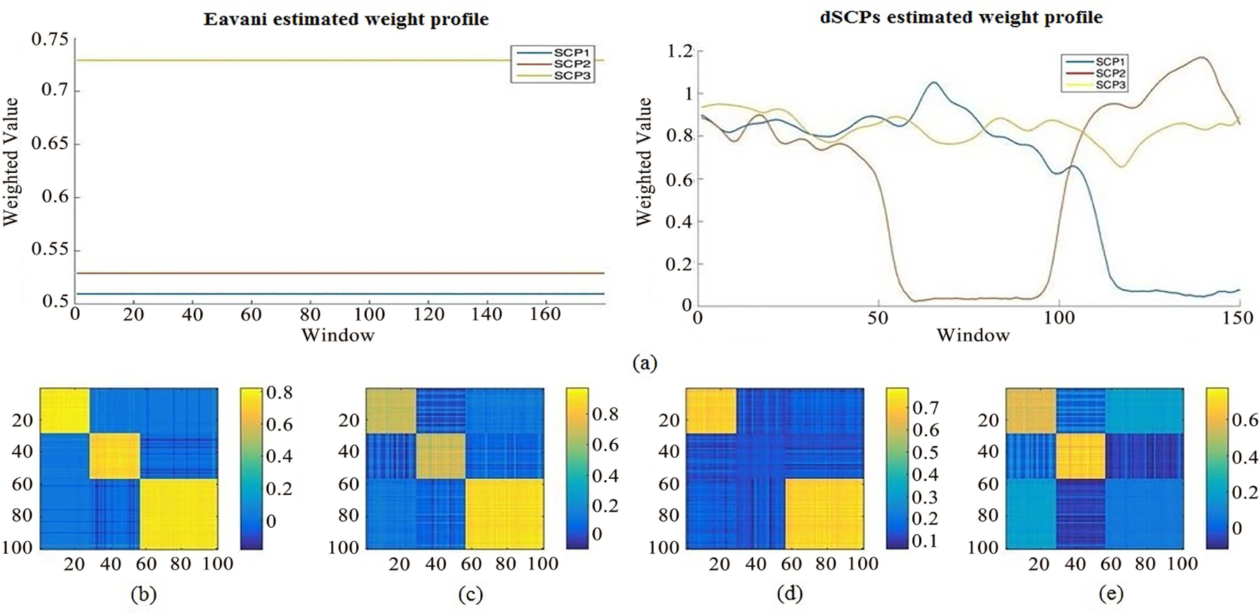
Analysis results for the simulated data using both static and proposed dynamic models.(a) The extraction of each SCP weighted values by Eavani et al.’s static model (left) and our dynamic method along the window sequences (right).(b) The correlation matrix reconstructed using Eavani et al.’s approach. (c-e) Three stages of reconstructed correlation matrices at different time period evaluated by the proposed method.

Fig.3(a) displays the alteration of weighted values along the window sequence for each SCP. This variation represents the change of SCP status between activated (”1”) or inactivated (”0”) in Fig.3(a). The real activated/inactivated status of the simulated data has been illustrated in Fig.2(b). Despite the presence of small variations, we can clearly observe that the estimated time evolution of the various weight values matches the ground truth fairly accurately.

On the other hand, when applying Eavani et al.’s method to synthetic data, only the static connectivity over the total period is displayed. As shown by the reconstructed matrix in Fig.3(b), we cannot detect the change of activation signal across time. By looking at Fig.3(c–e), our method can illuminate when the change in connectivity arrangements along the time course meets with the variation of the activation map. This example demonstrates that the estimation performed by our proposed model can accurately detect such changes in the BOLD time series signal.

In addition, we can further synthetical experiments when considering the case where some nodes may be shared among several SCPs. 4 SCPs were used while the various parameter values remained unchanged. Nodes 1−28 were part of networks 1, 2 and 4. Nodes 29−40 were shared by networks 3 and 4 and nodes 57 − 100 were correlated with networks 1 and 2. Both ground truth and analysis results for synthetic data can been seen in Fig.S2 in the supplementary materials. As shown in Fig.S2 (d)–(f), the reconstructed connectivity patterns coincided with the ground truth in Fig.S2 (a)–(c) very well.

B. Real dataset analysis

1). Data acquisition and preprocessing:

The Philadelphia Neurodevelopmental Cohort (PNC) is a large scale collaborative project between the Brain Behaviour Laboratory at the University of Pennsylvania and the Children’s Hospital of Philadelphia [30]. It is available via the dbGaP database, and contains resting state fMRI for nearly 900 adolescents with ages ranging from 8 to 21. Functional images were preprocessed using an automatic pipeline based on SPM 12 (http://www.fil.ion.ucl.ac.uk/spm/). The standard preprocessing steps include motion correction, spatial normalization to standard Montreal Neurological Institute (MNI) space and spatial smoothing with a 3mm FWHM Gaussian kernel. The influence of motion was further addressed using a regression procedure. A 0.01Hz - 0.1Hz band-pass filter was applied to the functional time series. Finally, the dimensionality of the data was reduced by making use of the standard 264 ROI templates as defined by Power et al. with a sphere radius parameter of 5mm [11]. Since we are interested in the development of brain connectivity with age, we divided the full dataset into two subsets based on age in months. Subjects whose age was over 210 months were sorted into the young adults group (age 18.99±1.12 years, 240 total subjects, 96 male and 146 female), while ages below 150 months were sorted into the child group (age 10.67 ± 1.09 years, 232 total subjects, 109 male and 123 female).

2). Tuning parameters for real data:

As stated above, three key parameters (the length of sliding window, the number of SCPs and the sparsity level of each SCP) need to be optimized to maximize the estimation power of our proposed framework when applied to resting state fMRI datasets. Both the window length l and sparsity level λ/p were estimated in terms of the reconstructed error depicted in Eq.6. In this case, λ/p is used instead of only λ, and the ROI number p equals 264 as defined by Power et al. [11]. Following the suggestions provided by Hutchison et al. [34] and Smith et al. [37], the minimal window length l needs to respect the following constraint:

$$l\ge \frac{1}{f_{\min }}$$ (7)

where f_min = 0.01Hz denotes the cutoff frequency by high-pass filtering. The shortest length window is above 50 TR(100s). Hence, the grid search for l and λ/p ranges from 40 to 70 and 0.01 to 1, respectively. Eavani et. al. selected d = 10 SCP and λ/p = 0.3 according to the reconstruction error [19]. Thus, when we optimized parameter l, d was set to 10. The optimization results are described in Fig.4(a) and (b). Fig.4(a) demonstrates that at point l = 50, we get the lowest reconstruction error averaged over several λ values, which agrees with the recommendation in references [34], [37]. Fig.4(b) reflects that the lowest error is reached for a sparsity level equals to 0.1.

Fig. 4.

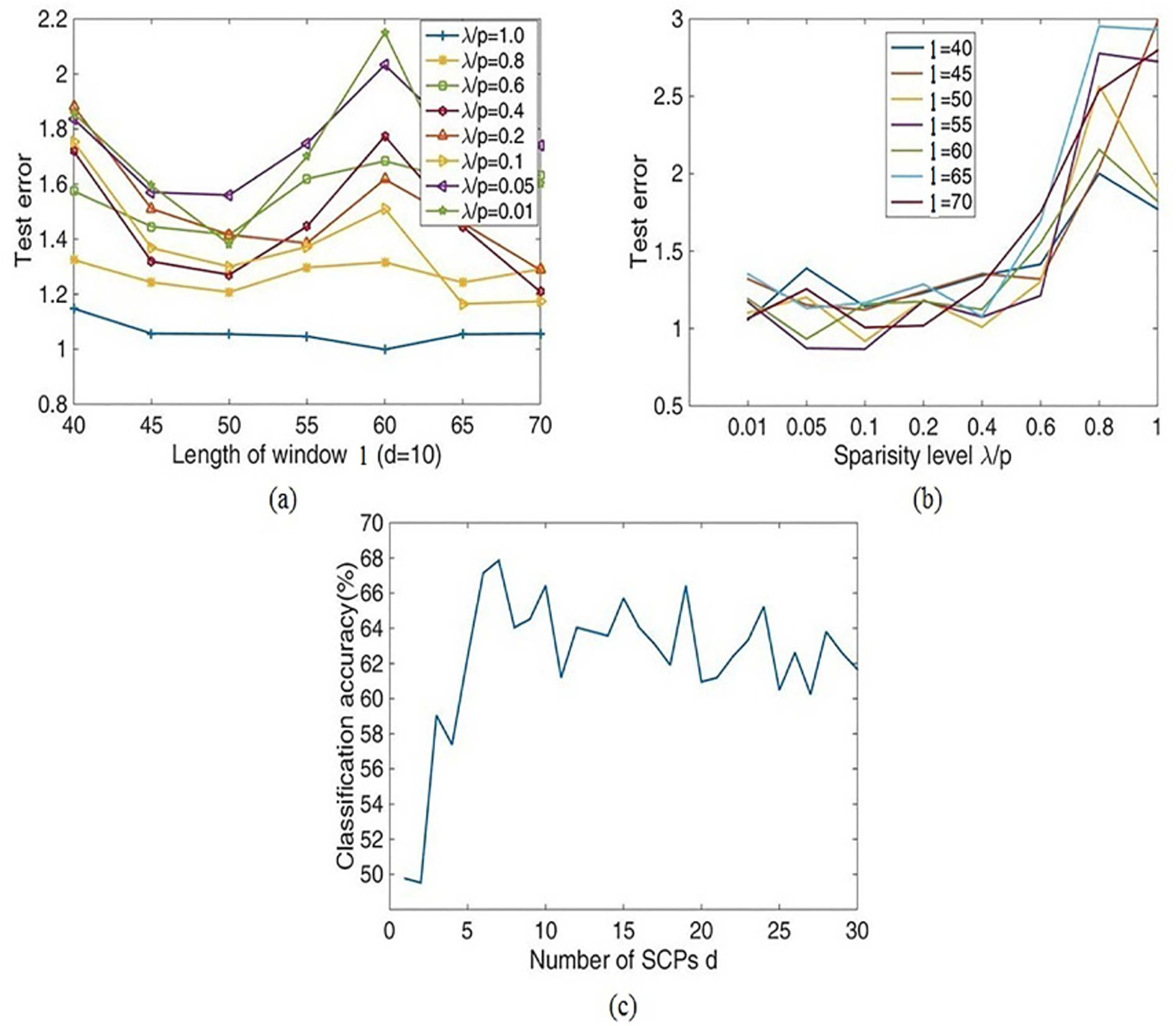
Optimization results for three key parameters in the dSCPs approach. (a) The reconstructed error for the length of window l across the test subjects (d = 10, l = 40, …, 70, λ/p = 0.01, …, 1). (b) The test error of sparsity level λ₁/p with the variation of the SCPs number (d = 10, l = 40, …, 70, λ/p = 0.01, …, 1). (c) The estimated results for the number of SCPs d based on the classification accuracy evaluated on the training/test subsets (l = 50, λ/p = 0.1, d = 1, …, 30).

The classification accuracy was used to determine the SCPs parameter number d. The candidate values ranged from 1 to 30. By applying the dSCPs model to both the training and testing subsets, we can extract the dynamic weighted matrices W_i,w, which were used as features. A linear kernel SVM was used for the classification step. Next, we carried out the entire procedure with 10 runs to estimate the reliability. The estimation results in Fig.4(c) represent that the accuracy first increases and then decreases as d increases. The highest classification accuracy was 67 ± 3.93% at d = 7. Thus, we chose to estimate d = 7 SCPs for the following investigation.

3). Postprocessing and results of resting state fMRI data:

For each subject, dynamic FC was estimated using the tapered sliding window approach with a length of 50 TR, resulting in n_w = 74 windows based on 1 TR step. We computed and concatenated the Pearson correlation matrices C_i,w, i = 1, 2 …, n, w = 1, 2 …, n_w from windowed segments as the input of dynamic SCPs. To facilitate the understanding of functional relationships within each state, we utilized data from Smith et al.’s study to assign 264 nodes into 10 functional networks corresponding to the primary resting state networks (RSNs) [40]. These networks included the medial visual network (”Med Vis”), occipital pole visual network (”OP Vis”), lateral visual network (”Lat Vis”), default mode network (”DMN”), cerebellum (”CB”), sensorimotor network (”SM”), auditory network (”Aud”), right frontoparietal network (”FPR”), left frontoparietal network (”FPL”) and executive control network (”EC”). According to Wang et al., 32 nodes are not strongly associated with any RSNs [41]. Thus, those nodes were not included in the following results. Implementing this method on the resting state fMRI dataset, we obtained 7 SCPs subnetworks with corresponding time varying weighted values. Interestingly, we found differences between children and young adults in distribution for some of the SCPs (two-sample Kolmogorov-Smirnov test with a significant level α = 0.01 is used to test if the weight values for a given SCP across both classes follow the same distribution [24]). The weight distribution of the 6th SCP, which had the strongest variation for these two subsets, is displayed in Fig.5(b). Other subnetworks which exhibited differences between the two groups are shown in Fig.S3 of supplementary materials. As shown in the histogram in Fig.5(b), the 6th SCP was significantly stronger within young adults than in children, as denoted by their class. Contributions from the lateral visual, occipital pole, auditory regions and the sensorimotor network were anti-correlated with both frontoparietal networks and the executive control map.

Fig. 5.

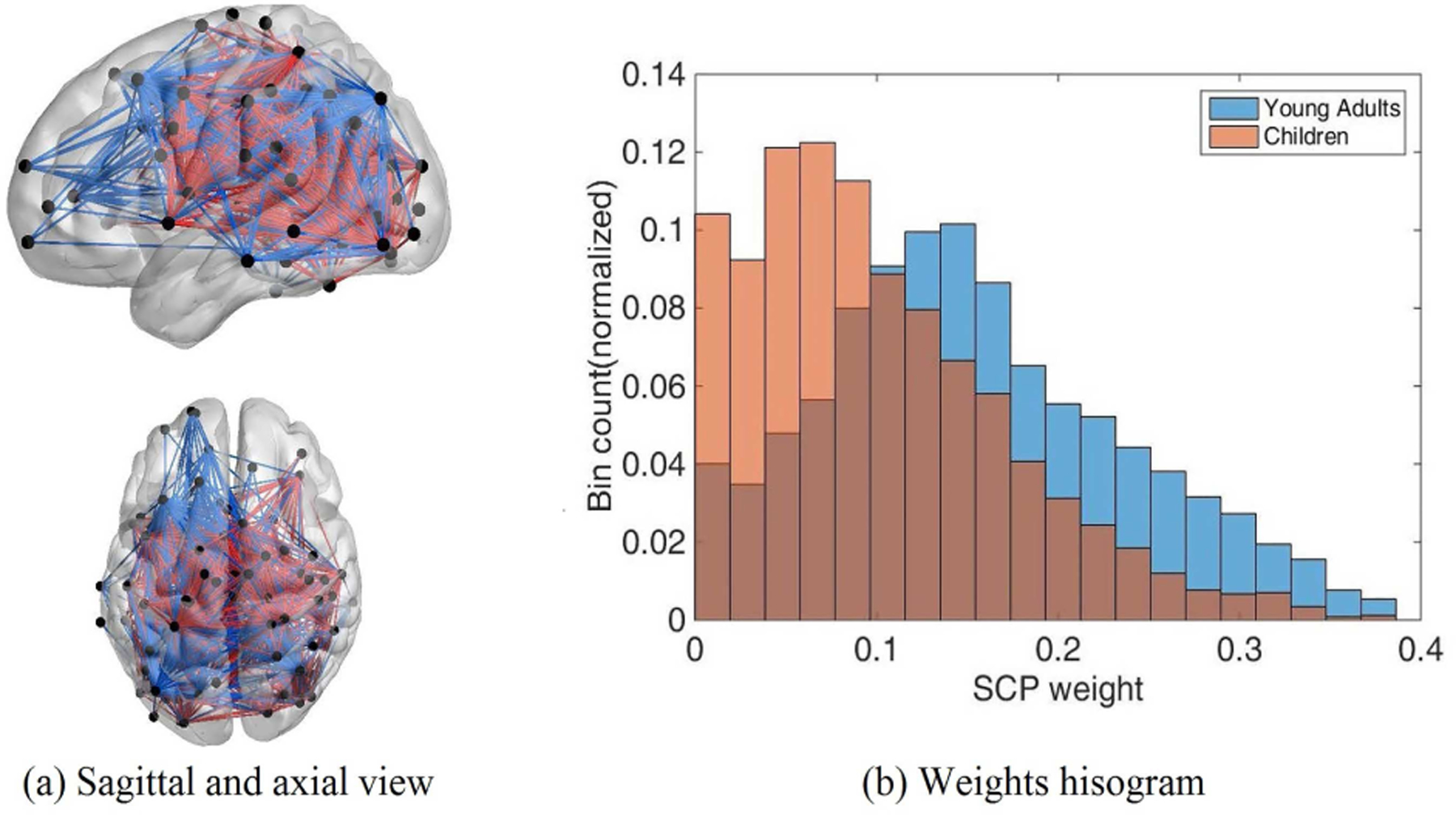
A visualization of the 6th SCP using BrainNet Viewer [42].(a) Sagittal and axial view for the 6th SCP subnetwork. (b) Weights of this SCP within each class.

In order to explain the difference between these two groups based on the time varying weights, the following postprocessing steps were carried out. For assessing the frequency and reoccurring patterns of FC, k-means clustering [6] was applied to dynamic weighted matrices. Specifically, we treated weighted matrix $W_{in}\in {ℝ}^{d\times N}$, N = i × n_w as the input, which reflects time-varying alteration of connectivity. We estimated the optimal number of dynamic FC states (centroids) to be 4 using the elbow criterion defined as the ratio of within-cluster distance to between-cluster distance shown in Fig.6. The centroids were diagonal matrices $W_k\in {ℝ}^{d\times d}$, k = 1, 2, 3, 4 and can represent the reoccurring patterns of FC through reconstructed correlation matrices $C_k\in {ℝ}^{p\times p}$ using the SCPs vectors x. At first, the clustering was performed on a subset of windows for each subject, which had local maxima in weights variance [6]. The initial results were named as exemplars and set as starting points to cluster all the dynamic weighted data. After obtaining the centroids of both classes, we reconstructed the correlation matrix for each state making use of the SCPs vectors x.

Fig. 6.

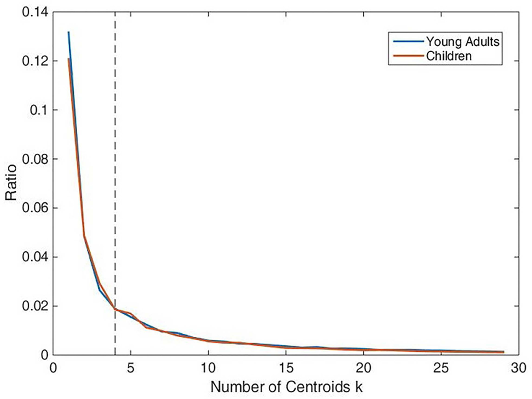
Elbow criterion for selecting the number of centroids of k-means clustering.

By employing k-means clustering based on dynamic weighted matrices, four dynamic FC states for each group were identified, which reoccurred throughout the scan and across subjects. Dynamic states for the two classes, young adult and children, are shown in Fig.7. We observe that, from state 1 to state 4, the overall correlation gradually became stronger. States 1 and 2 can be characterized as unconnected due to the weak connectivity intensity between functional networks. By contrast, states 3 and 4 can be characterized as connected via the same criteria. It is interesting to note that the unconnected states were detected more frequently than the connected ones; that is, given a larger time period, the connectivity of the human brain relies on relatively unconnected conditions.

Fig. 7.

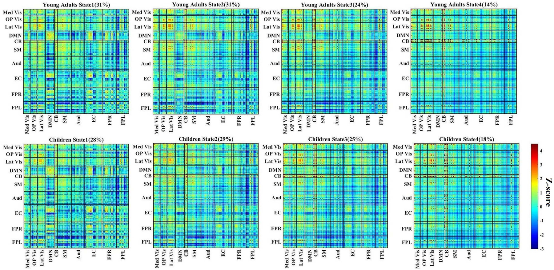
Dynamic functional connectivity (FC) states for the young adult (top) and children (bottom) groups (z-scores). Dynamic FC states were derived from k-means clustering using the SCPs vectors. Total percentage of occurrence for each state is listed above each picture. Following Smith et al.’s work, the resting state networks (RSNs) were divided into 10 major functional subnetworks [40].

To further assess group differences in dynamic connectivity, an element-wise subject median was computed for each state using each subject’s windowed correlation matrices. In this way, the median matrix can be considered as the representative pattern of the subject for a particular state [28]. The visualization of medians for each state across the two groups is depicted in Fig.8(A). Note that not all subjects have dynamic windows that are assigned to every state, thus the count of observations varies with the state (see the subject counts on the top of Fig.8(A)). Following the pipeline provided by Elena et al., univariate analysis was used on these subject median matrices to investigate the association of connectivity with age [4]. The univariate model was defined as follows:

$$\tilde{K}=D\beta$$ (8)

where β is the linear regression coefficient and D denotes the design matrix consisting of the age of subjects. Here, age was log-transformed to improve symmetry and reduce the disproportionate influence of outlier values on the univariate model fit. $\tilde{K}$ represents the response variables. For each i ∈ 1, 2, …, n subjects, we expand its subject median matrix $M_i^{p\times p}$ into a one dimensional vector, $K_i^{1\times P}$, P = p × p. Prior to modeling, response variables were Fisher-transformed [z = atanh(k)]. Then, the response matrices were constructed by concatenating the response vectors: $\tilde{K}={\left[atanh\left(K_1^T\right),\dots ,atanh\left(K_n^T\right)\right]}^T$. A two-sample t-test was performed on the regression coefficients across the subject median dynamic FC matrices by state, using a q = 0.05 significance level. The group modifications were visualized through plotting the log of p value with the sign of t statistics,−sign(t)log₁₀(p).

Fig. 8.

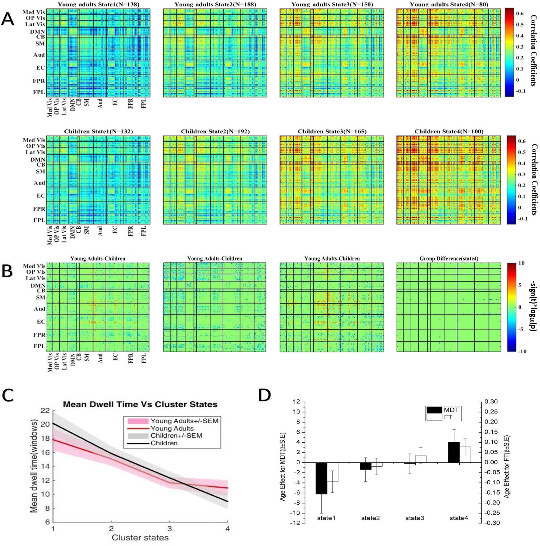
A) The medians of cluster centroids for the young adult (top) and child groups (middle), with the count of subjects which have at least one window for each state displayed. Not all subjects entered all states during the scanning time period. Hence, the number of subjects in each state for two groups is below the total number (240 for the young adult group and 232 for children group). B) Group variation was visualized by plotting the log of p value with the sign of t statistics, −sign(t)log₁₀(p). The two-sample t-test is performed on the regression coefficients across the subject median dynamic FC maps by state and FDR corrected (q < 0.05). C) The mean± error of dwell times by each state for young adults (red) and children (black). D) Summary from four dynamic FC matrices associated with age. Positive value of β means that the older group spends more time in the corresponding state. Meanwhile, negative value of β indicates that the younger group spends more time in that state.

The significant group differences in functional subnetworks among these four identified states are depicted in Fig.8(B). Although the human brain shows the most intense activity in state 4, the group differences in states 1, 2, 3 were much stronger than in state 4. The details are discussed as follows. Essentially, as shown in Fig.8(B), all relationships between the DMN and other subnetworks are reported to have increased connectivity in children in contrast with young adults. In addition to DMN, networks EC, FPR and FPL also had powerful correlations within the CB network.

States 1 and 3 within the visual system had displayed increased intensity young adults, which agreed with the results from a study by Jolles et al., who showed overall lower connectivity in the visual system for children [43]. However, it should be noted that young children had higher connectivity within the visual system in state 2, but we were unable to detect significant variations in state 4. The results from states 1 and 3 also suggested that young adults had increased connectivity in the SM, Aud and EC relative to children group. Interestingly, as age increased, positive influence on the correlation between the visual systems, SM, Aud and EC in states 1 and 3 appeared.

In addition to these results, both frontoparietal networks showed slightly increased connectivity with the visual system, SM, Aud and EC of children. More specifically, the weakest variation of correlation between children and young adults for these networks is in state 4. The difference gradually increases from state 3 to state 1, then to state 2.

To investigate the time occupied by each state and the effect of age, the summary measures, including mean dwell time (MDT) and fraction of time (FT), were estimated from the state transition vector. The definition of MDT and FT for each subject was provided by Blanken et al. [44].

$$\begin{gathered} MD{T}^{state\left(k\right)}=mean\left(T{R}_{end}-T{R}_{start}\right) \\ F{T}^{state\left(k\right)}=\frac{sum{\left(state\_vector\right)}^{subject\left(i\right)}==1}{Total\hspace{0.17em}Number\hspace{0.17em}of\hspace{0.17em}TR} \end{gathered}$$ (9)

where TR_start and TR_end are evaluated through the following equations, i ∈ 1, 2, …, n. ”1” and ”−1” mean that the specific window belongs to a certain state or not [44].

$$\begin{gathered} T{R}_{start}=count\left(difference\left(state\_vecto{r}_{subject\left(i\right)},state\_number\right)==1\right) \\ T{R}_{end}=count\left(difference\left(state\_vecto{r}_{subject\left(i\right)},state\_number\right)==-1\right) \end{gathered}$$ (10)

Fig.8(C) shows the proportion of subject windows assigned to each state for both groups. The result showed that young adults spend more time in state 4 and less time in state 1 (paired samples t-test with a significant level α = 0.05 is used). Compared to children, young adults make more transitions to state 4, which is the most connected state. This demonstrates the effect of age on dwell time for each state. To further investigate the effect of age, statistical analyses using a univariate linear regression model were carried out on MDT and FT. The parameter β stands for linear regression coefficient. In Fig.8(D), a positive value of β shows that the older group spends more time in the corresponding state relative to children, and a negative coefficient of β indicates that children spend more time in that particular state. Using the value of β for MDT and FT, we found that age had the most significant influence on state 1 and state 4 (p − value ≤ 0.05). The results indicated that young adults spent more time in the relatively active state (state 4). However, this was reversed in state 1 for the children.

IV. Discussion

In this study, we presented a computational approach, namely dSCPs, for the estimation of dynamic network connectivity patterns, which extends the static model of Eavani et al. [19]. This new data-driven approach utilizes a sliding window technique [6]. Specifically, we examined fMRI data to study the dynamics of functional connectivity with a sparse regression model. We first validated the feasibility of our approach using simulated experiments, and then optimized the key parameters within the sparse regression model in terms of the reconstruction error. We then investigated the difference in dynamic functional connectivity between young adults and children using real resting state fMRI data from the PNC.

Our simulated experiments showed the feasibility of the proposed approach. In contrast to the existing static models, our approach can detect dynamic changes in fMRI signals more accurately, demonstrating its power in analyzing the time-varying functional connectivity of human brains.

Furthermore, our dynamic model was used to study the differences between young adults and children in a relatively large sample of participants in the PNC study (n = 472). The network dynamics extracted by our approach indicated that some connectivities remained in almost all dynamic states with various strengths. We propose that this is due to the fact that functional connectivity networks do not change dramatically, but rather gradually through brain development as age increases. This observation matches with the research proposed by Marek et al. [45].

We found clear differences between young adults and children. Four highly reoccurring dynamic FC states were extracted and evaluated statistically. Our analyses suggested that, compared with young adults, children have increased connectivity between DMN and other subnetworks. Hutchison et al. performed a similar dynamic connectivity study with a smaller sample (N=51) and applied the Group ICA approach [46]. They found that children had stronger connectivity between DMN and the cognitive control system, which is in line with our discovery. In addition, we found that children have hypoconnectivity within the visual system in states 1 and 3 and greater connectivity in state 2. Interestingly, Jolles et al. have reported that there is an increased connectivity in visual system for young adults compared to children [43]. Meanwhile, we observed that children reveal reduced connectivity among the SM, EC and Aud for states 1 and 3. This is in accord with several recent studies [4], [47], [48] that found that brain circuitry moves from segregation to integration with increasing age. In addition, children also had stronger connectivity between both frontoparietal subnetworks and the visual system, SM, Aud, CB and EC. Finally, hyperconnectivity between the DMN, Aud and EC in children compared with young adults was also observed, which was in agreement with the results of a similar study by Jolles et al. [43].

In sum, we have demonstrated that there is an age-related influence on the time spent in dynamic functional states across the groups. Specifically, we observed that young adults spend more time in state 4, which was the most connected connectivity pattern. By comparison, children tend to spend more time in the relatively disconnected connectivity pattern of state 1. This is in line with what has been reported previously [49], [50].

To date, the most commonly used strategy for examining dynamic connectivity in rsfMRI has been the sliding window approach combined with Group ICA at the voxel level [6], [25], [28], [31], [34], [46]. This ICA-based approach assumes independence of components to derive spatial patterns. Within this framework, whole brain data are subjected to Group ICA to identify brain connectivity networks. Subsequently, a clustering approach is utilized to observe distinct and repeatable FC patterns from rsfMRI.

Compared with the Group ICA method, which reduces data dimensions using PCA, our approach performs the analysis on input data directly. In regard to computational time, our approach works for data at the ROIs level, but would be more complicated at the voxel level. Furthermore, our model does not assume a relationship between brain states. With sparsity enforcement, our analysis results will contain both dynamic information and sparse connectivity networks, which can be easily interpreted as in [19]. To reveal dynamic FC, a clustering method like that used in ICA must also be implemented in our method. Of note, a recent study used the Group ICA approach on 146 children [31]. This study found that children of different ages spent various time in certain FC states, and that variability in FC increased with age. These results are concordant with ours using the PNC dataset mentioned above.

One potential limitation of the proposed model is the SCP number selection, or determining the appropriate value for d. While model selection remains an open and difficult problem, it is vital for the result. We use cross-validation for optimizing the value of d in terms of subsequent classification accuracy, which was practical for our analysis. In addition, Pearson correlation was used in this study for connectivity analysis and other ways such as partial correlation can also be applied. Besides that, we can also use other regularization terms, such as generalized fused Lasso, in our regression model, and compare their capabilities in uncovering network dynamics [24]. Finally, in our ongoing work, we begin to perform a systematic comparison between our proposed model and other comparable dynamic connectivity methods. We will also test on different datasets such as PING study (http://pingstudy.ucsd.edu/) with the same preprocessing steps. The results will be reported elsewhere.

V. Conclusion

We propose an approach named dSCPs to extract sparse co-activated subnetworks from rsfMRI data. We applied an optimization algorithm based on ADMM for solving the model. In addition, we performed model selection and optimize key parameters in the model using cross-validation in terms of classification accuracy. Both simulated and real data were used to show the validity and feasibility of our model for dynamic connectivity analysis. Results for the FC network difference between young adults and children from the PNC dataset were consistent with existing studies, demonstrating temporal correlations within functional subnetworks. In particular, we showed that young adults tend to spend more time in the relatively stationary connectivity patterns relative to children. In summary, we demonstrated that the dSCPs estimated using our model can facilitate the extraction of dynamic functional connectivity networks for the study of complex brain dynamics, where connectivity patterns are widely regarded as important biomarkers.

References

- [1].Du Y, Liu J, Sui J, He H, Pearlson GD, and Calhoun VD, “Exploring difference and overlap between schizophrenia, schizoaffective and bipolar disorders using resting-state brain functional networks,” in Engineering in Medicine and Biology Society (EMBC), 2014 36th Annual International Conference of the IEEE. IEEE, 2014, pp. 1517–1520. [DOI] [PubMed] [Google Scholar]
- [2].Du Y, Pearlson GD, Liu J, Sui J, Yu Q, He H, Castro E, and Calhoun VD, “A group ica based framework for evaluating resting fmri markers when disease categories are unclear: application to schizophrenia, bipolar, and schizoaffective disorders,” NeuroImage, vol. 122, pp. 272–280, 2015. [DOI] [PMC free article] [PubMed] [Google Scholar]
- [3].Khadka S, Meda SA, Stevens MC, Glahn DC, Calhoun VD, Sweeney JA, Tamminga CA, Keshavan MS, ONeil K, Schretlen D et al. , “Is aberrant functional connectivity a psychosis endophenotype? a resting state functional magnetic resonance imaging study,” Biological psychiatry, vol. 74, no. 6, pp. 458–466, 2013. [DOI] [PMC free article] [PubMed] [Google Scholar]
- [4].Allen EA, Erhardt EB, Damaraju E, Gruner W, Segall JM, Silva RF, Havlicek M, Rachakonda S, Fries J, Kalyanam R et al. , “A baseline for the multivariate comparison of resting-state networks,” Frontiers in systems neuroscience, vol. 5, p. 2, 2011. [DOI] [PMC free article] [PubMed] [Google Scholar]
- [5].Qin J, Chen S-G, Hu D, Zeng L-L, Fan Y-M, Chen X-P, and Shen H, “Predicting individual brain maturity using dynamic functional connectivity,” Frontiers in human neuroscience, vol. 9, p. 418, 2015. [DOI] [PMC free article] [PubMed] [Google Scholar]
- [6].Allen EA, Damaraju E, Plis SM, Erhardt EB, Eichele T, and Calhoun VD, “Tracking whole-brain connectivity dynamics in the resting state,” Cerebral cortex, p. bhs352, 2012. [DOI] [PMC free article] [PubMed] [Google Scholar]
- [7].Raichle M, “The restless brain. brain connect. 1, 3–12. 10.1089/brain, 2011. [DOI] [PMC free article] [PubMed] [Google Scholar]
- [8].Posse S, Ackley E, Mutihac R, Zhang T, Hummatov R, Akhtari M, Chohan MO, Fisch B, and Yonas H, “High-speed real-time resting-state fmri using multi-slab echo-volumar imaging,” Frontiers in human neuroscience, vol. 7, p. 479, 2013. [DOI] [PMC free article] [PubMed] [Google Scholar]
- [9].Buckner R, Andrews-Hanna J, and Schacter D, “The brains default network: anatomy, function, and relevance to disease ann ny acad sci 2008; 1124: 1–38.” [DOI] [PubMed] [Google Scholar]
- [10].Rosvall M and Bergstrom CT, “Maps of random walks on complex networks reveal community structure,” Proceedings of the National Academy of Sciences, vol. 105, no. 4, pp. 1118–1123, 2008. [DOI] [PMC free article] [PubMed] [Google Scholar]
- [11].Power JD, Cohen AL, Nelson SM, Wig GS, Barnes KA, Church JA, Vogel AC, Laumann TO, Miezin FM, Schlaggar BL et al. , “Functional network organization of the human brain,” Neuron, vol. 72, no. 4, pp. 665–678, 2011. [DOI] [PMC free article] [PubMed] [Google Scholar]
- [12].Calhoun VD, Liu J, and Adalı T, “A review of group ica for fmri data and ica for joint inference of imaging, genetic, and erp data,” Neuroimage, vol. 45, no. 1, pp. S163–S172, 2009. [DOI] [PMC free article] [PubMed] [Google Scholar]
- [13].Anderson A, Douglas PK, Kerr WT, Haynes VS, Yuille AL, Xie J, Wu YN, Brown JA, and Cohen MS, “Non-negative matrix factorization of multimodal mri, fmri and phenotypic data reveals differential changes in default mode subnetworks in adhd,” NeuroImage, vol. 102, pp. 207–219, 2014. [DOI] [PMC free article] [PubMed] [Google Scholar]
- [14].Zhou Z, Ding M, Chen Y, Wright P, Lu Z, and Liu Y, “Detecting directional influence in fmri connectivity analysis using pca based granger causality,” Brain research, vol. 1289, pp. 22–29, 2009. [DOI] [PMC free article] [PubMed] [Google Scholar]
- [15].Aharon M, Elad M, and Bruckstein A, “rmk-svd: An algorithm for designing overcomplete dictionaries for sparse representation,” IEEE Transactions on signal processing, vol. 54, no. 11, pp. 4311–4322, 2006. [Google Scholar]
- [16].Lee K, Tak S, and Ye JC, “A data-driven sparse glm for fmri analysis using sparse dictionary learning with mdl criterion,” IEEE Transactions on Medical Imaging, vol. 30, no. 5, pp. 1076–1089, 2011. [DOI] [PubMed] [Google Scholar]
- [17].Lv J, Jiang X, Li X, Zhu D, Zhang S, Zhao S, Chen H, Zhang T, Hu X, Han J et al. , “Holistic atlases of functional networks and interactions reveal reciprocal organizational architecture of cortical function,” IEEE Transactions on Biomedical Engineering, vol. 62, no. 4, pp. 1120–1131, 2015. [DOI] [PubMed] [Google Scholar]
- [18].Lv J, Lin B, Li Q, Zhang W, Zhao Y, Jiang X, Guo L, Han J, Hu X, Guo C et al. , “Task fmri data analysis based on supervised stochastic coordinate coding,” Medical image analysis, vol. 38, pp. 1–16, 2017. [DOI] [PMC free article] [PubMed] [Google Scholar]
- [19].Eavani H, Satterthwaite TD, Filipovych R, Gur RE, Gur RC, and Davatzikos C, “Identifying sparse connectivity patterns in the brain using resting-state fmri,” Neuroimage, vol. 105, pp. 286–299, 2015. [DOI] [PMC free article] [PubMed] [Google Scholar]
- [20].Hoff PD, “A hierarchical eigenmodel for pooled covariance estimation,” Journal of the Royal Statistical Society: Series B (Statistical Methodology), vol. 71, no. 5, pp. 971–992, 2009. [Google Scholar]
- [21].Kolda TG and Bader BW, “Tensor decompositions and applications,” SIAM review, vol. 51, no. 3, pp. 455–500, 2009. [Google Scholar]
- [22].Wang H, Banerjee A, and Boley D, “Common component analysis for multiple covariance matrices,” in Proceedings of the 17th ACM SIGKDD international conference on Knowledge discovery and data mining. ACM, 2011, pp. 956–964. [Google Scholar]
- [23].Lee E, “Advanced bayesian models for high-dimensional biomedical data,” Ph.D. dissertation, The University of North Carolina at Chapel Hill, 2016. [Google Scholar]
- [24].Zille P, Calhoun VD, Stephen JM, Wilson TW, and Wang YP, “Fused estimation of sparse connectivity patterns from rest fmri. application to comparison of children and adult brains,” IEEE Transactions on Medical Imaging, vol. PP, no. 99, pp. 1–1, 2017. [DOI] [PMC free article] [PubMed] [Google Scholar]
- [25].Calhoun VD, Miller R, Pearlson G, and Adalı T, “The chronnectome: time-varying connectivity networks as the next frontier in fmri data discovery,” Neuron, vol. 84, no. 2, pp. 262–274, 2014. [DOI] [PMC free article] [PubMed] [Google Scholar]
- [26].Hutchison RM, Womelsdorf T, Gati JS, Everling S, and Menon RS, “Resting-state networks show dynamic functional connectivity in awake humans and anesthetized macaques,” Human brain mapping, vol. 34, no. 9, pp. 2154–2177, 2013. [DOI] [PMC free article] [PubMed] [Google Scholar]
- [27].Abrol A, Chaze C, Damaraju E, and Calhoun VD, “The chronnectome: Evaluating replicability of dynamic connectivity patterns in 7500 resting fmri datasets,” in Engineering in Medicine and Biology Society (EMBC), 2016 IEEE 38th Annual International Conference of the. IEEE, 2016, pp. 5571–5574. [DOI] [PubMed] [Google Scholar]
- [28].Damaraju E, Allen E, Belger A, Ford J, McEwen S, Mathalon D, Mueller B, Pearlson G, Potkin S, Preda A et al. , “Dynamic functional connectivity analysis reveals transient states of dysconnectivity in schizophrenia,” NeuroImage: Clinical, vol. 5, pp. 298–308, 2014. [DOI] [PMC free article] [PubMed] [Google Scholar]
- [29].Rashid B, Damaraju E, Pearlson GD, and Calhoun VD, “Dynamic connectivity states estimated from resting fmri identify differences among schizophrenia, bipolar disorder, and healthy control subjects,” Frontiers in human neuroscience, vol. 8, p. 897, 2014. [DOI] [PMC free article] [PubMed] [Google Scholar]
- [30].Satterthwaite TD, Connolly JJ, Ruparel K, Calkins ME, Jackson C, Elliott MA, Roalf DR, Hopson R, Prabhakaran K, Behr M et al. , “The philadelphia neurodevelopmental cohort: A publicly available resource for the study of normal and abnormal brain development in youth,” Neuroimage, vol. 124, pp. 1115–1119, 2016. [DOI] [PMC free article] [PubMed] [Google Scholar]
- [31].Marusak HA, Calhoun VD, Brown S, Crespo LM, Sala-Hamrick K, Gotlib IH, and Thomason ME, “Dynamic functional connectivity of neurocognitive networks in children,” Human Brain Mapping, vol. 38, no. 1, pp. 97–108, 2017. [DOI] [PMC free article] [PubMed] [Google Scholar]
- [32].Boyd S, Parikh N, Chu E, Peleato B, and Eckstein J, “Distributed optimization and statistical learning via the alternating direction method of multipliers,” Foundations and Trends® in Machine Learning, vol. 3,, no. 1, pp. 1–122, 2011. [Google Scholar]
- [33].Danaher P, Wang P, and Witten DM, “The joint graphical lasso for inverse covariance estimation across multiple classes,” Journal of the Royal Statistical Society: Series B (Statistical Methodology), vol. 76, no. 2, pp. 373–397, 2014. [DOI] [PMC free article] [PubMed] [Google Scholar]
- [34].Hutchison RM, Womelsdorf T, Allen EA, Bandettini PA, Calhoun VD, Corbetta M, Della Penna S, Duyn JH, Glover GH, Gonzalez-Castillo J et al. , “Dynamic functional connectivity: promise, issues, and interpretations,” Neuroimage, vol. 80, pp. 360–378, 2013. [DOI] [PMC free article] [PubMed] [Google Scholar]
- [35].Sakoǧlu Ü, Pearlson GD, Kiehl KA, Wang YM, Michael AM, and Calhoun VD, “A method for evaluating dynamic functional network connectivity and task-modulation: application to schizophrenia,” Magnetic Resonance Materials in Physics, Biology and Medicine, vol. 23, no. 5–6, pp. 351–366, 2010. [DOI] [PMC free article] [PubMed] [Google Scholar]
- [36].Chang C and Glover GH, “Time–frequency dynamics of resting-state brain connectivity measured with fmri,” Neuroimage, vol. 50, no. 1, pp. 81–98, 2010. [DOI] [PMC free article] [PubMed] [Google Scholar]
- [37].Smith SM, Miller KL, Moeller S, Xu J, Auerbach EJ, Woolrich MW, Beckmann CF, Jenkinson M, Andersson J, Glasser MF et al. , “Temporally-independent functional modes of spontaneous brain activity,” Proceedings of the National Academy of Sciences, vol. 109, no. 8, pp. 3131–3136, 2012. [DOI] [PMC free article] [PubMed] [Google Scholar]
- [38].Cortes C and Vapnik V, “Support-vector networks,” Machine learning, vol. 20, no. 3, pp. 273–297, 1995. [Google Scholar]
- [39].Erhardt EB, Allen EA, Wei Y, Eichele T, and Calhoun VD, “Simtb, a simulation toolbox for fmri data under a model of spatiotemporal separability,” Neuroimage, vol. 59, no. 4, pp. 4160–4167, 2012. [DOI] [PMC free article] [PubMed] [Google Scholar]
- [40].Smith SM, Miller KL, Salimi-Khorshidi G, Webster M, Beckmann CF, Nichols TE, Ramsey JD, and Woolrich MW, “Network modelling methods for fmri,” Neuroimage, vol. 54, no. 2, pp. 875–891, 2011. [DOI] [PubMed] [Google Scholar]
- [41].Wang Y, Kang J, Kemmer PB, and Guo Y, “An efficient and reliable statistical method for estimating functional connectivity in large scale brain networks using partial correlation,” Frontiers in neuroscience, vol. 10, 2016. [DOI] [PMC free article] [PubMed] [Google Scholar]
- [42].Xia M, Wang J, and He Y, “Brainnet viewer: a network visualization tool for human brain connectomics,” PloS one, vol. 8, no. 7, p. e68910, 2013. [DOI] [PMC free article] [PubMed] [Google Scholar]
- [43].Jolles DD, van Buchem MA, Crone EA, and Rombouts SA, “A comprehensive study of whole-brain functional connectivity in children and young adults,” Cerebral cortex, vol. 21, no. 2, pp. 385–391, 2011. [DOI] [PubMed] [Google Scholar]
- [44].Blanken L, On the Spectrum: the neurobiology of psychiatric symptoms in the general population. Erasmus University Rotterdam, 2016. [Google Scholar]
- [45].Marek S, Hwang K, Foran W, Hallquist MN, and Luna B, “The contribution of network organization and integration to the development of cognitive control,” PLoS biology, vol. 13, no. 12, p. e1002328, 2015. [DOI] [PMC free article] [PubMed] [Google Scholar]
- [46].Hutchison RM and Morton JB, “Tracking the brain’s functional coupling dynamics over development,” Journal of Neuroscience, vol. 35, no. 17, pp. 6849–6859, 2015. [DOI] [PMC free article] [PubMed] [Google Scholar]
- [47].Dosenbach NU, Nardos B, Cohen AL, Fair DA, Power JD, Church JA, Nelson SM, Wig GS, Vogel AC, Lessov-Schlaggar CN et al. , “Prediction of individual brain maturity using fmri,” Science, vol. 329, no. 5997, pp. 1358–1361, 2010. [DOI] [PMC free article] [PubMed] [Google Scholar]
- [48].Anderson JS, Nielsen JA, Froehlich AL, DuBray MB, Druzgal TJ, Cariello AN, Cooperrider JR, Zielinski BA, Ravichandran C, Fletcher PT et al. , “Functional connectivity magnetic resonance imaging classification of autism,” Brain, vol. 134, no. 12, pp. 3742–3754, 2011. [DOI] [PMC free article] [PubMed] [Google Scholar]
- [49].Fair DA, Cohen AL, Dosenbach NU, Church JA, Miezin FM, Barch DM, Raichle ME, Petersen SE, and Schlaggar BL, “The maturing architecture of the brain’s default network,” Proceedings of the National Academy of Sciences, vol. 105, no. 10, pp. 4028–4032, 2008. [DOI] [PMC free article] [PubMed] [Google Scholar]
- [50].Zuo X-N, Kelly C, Di Martino A, Mennes M, Margulies DS, Bangaru S, Grzadzinski R, Evans AC, Zang Y-F, Castellanos FX et al. , “Growing together and growing apart: regional and sex differences in the lifespan developmental trajectories of functional homotopy,” Journal of Neuroscience, vol. 30, no. 45, pp. 15 034–15 043, 2010. [DOI] [PMC free article] [PubMed] [Google Scholar]
Associated Data
This section collects any data citations, data availability statements, or supplementary materials included in this article.