Describing the COVID-19 outbreak during the lockdown: fitting modified SIR models to data

Abstract

In this paper, we analyse the COVID-19 outbreak data with simple modifications of the SIR compartmental model, in order to understand the time evolution of the cases in Italy and Germany, during the first half of 2020. Even if the complexity of the pandemic cannot be easily described, we show that our models are suitable for understanding the data during the application of the social distancing and the lockdown. We compare and contrast different modifications of the SIR model showing the strengths and the weaknesses of each approach. Finally, we discuss the reliability of the model predictions for estimating the near- and far-future evolution of the outbreak.

Introduction

The Coronavirus Disease, named COVID-19, is an infectious disease caused by the newly discovered coronavirus SARS-CoV-2 [1]. Most people infected with the COVID-19 virus experiences from mild to moderate respiratory illness and recover without requiring special treatment. Older people and those with underlying pre-existing medical problems like cardiovascular diseases, diabetes, chronic respiratory diseases, and cancer are more likely to develop serious illness. Yet, at present much needs to be understood about the effects of this new virus. COVID-19 spreads quickly, mainly through droplets of saliva or discharge from the nose when an infected person coughs or sneezes. The coronavirus inside airborne droplets can survive for many tens of minutes and eventually sticks to surfaces and remains active up to many hours, depending on materials [2]. This fact could further increase the diffusion of the outbreak.

The velocity of the outbreak spread is described by the so-called basic reproduction number (or ratio), usually referred to as $R_0$, defined as the expected number of new infections from a single new case in a population where all subjects are susceptible. The lockdown and/or the social distancing should help in reducing $R_0$, making the outbreak duration shorter than the typical time needed by the free natural evolution until the so-called herd immunity is reached.

Another important feature of COVID-19, and in general for outbreaks in progress, is the impossibility of quantifying the asymptomatic population. Many ongoing studies, as, for example, [3], are indeed showing that this component could be a substantial fraction of the visible cases, i.e. the ones detected by reliable medical tests. Even if not detected, the asymptomatic cases can play an important role in the diffusion of the coronavirus epidemic and can drastically change the outcome of the model predictions. In this work, we infer $R_0$ and other parameters from data and discuss the evolution of the outbreak during the lockdown, analysing simultaneously the cumulative behaviour of active and removed (namely “recovered plus deceased”) cases, using the additive least square method.

In Sect. 2, we introduce a time dependence of the parameters of the standard SIR compartmental model. In Sect. 3, we introduce a change in the model to account for recovered and deceased compartments separately. In Sect. 4, we discuss results for Italian data. In Sect. 5, we discuss results for Germany as an example of application to other dataset. Finally, in Sect. 6 we present a model accounting for the asymptomatic hidden component that is not yet detected for various practical reasons. In Sect. 7, we draw our conclusions.

SIR-T: a time-dependent SIR model

From SIR to SIR-T

In order to study the spread of the COVID-19, we take into account the basic SIR model [4]. In the model, we distinguish three categories of individuals, known as “compartments”: S for the number of susceptible, I for the number of infectious and R for the number of recovered. The last category might include recovered and deceased together or separately. Based on this assumption, the mathematical model is written in terms of the following set of differential equations:

$$\begin{array}{c}\hfill \begin{array}{cc}\hfill \frac{\mathrm{d}S(t)}{\mathrm{d}t}& =-\beta \frac{S(t)I(t)}{N}\hfill \\ \hfill \frac{\mathrm{d}I(t)}{\mathrm{d}t}& =\beta \frac{S(t)I(t)}{N}-\gamma I(t)\hfill \\ \hfill \frac{\mathrm{d}R(t)}{\mathrm{d}t}& =\gamma I(t)\hfill \\ \hfill \end{array}\end{array}$$ 1

where $N=S(t)+I(t)+R(t)$ is constant by definition being zero the sum of their derivatives, $\beta$ determines the transmission rate and $\gamma$ is the recovery rate. If a susceptible population of ($S(t=0)=N$) people is affected for the first time by the outbreak, the initial conditions of the system (1) can be easily cast as: $N(0)=N_0$, $I(0)=I_0$ and $R(0)=0$.

In the SIR model, the $R_0$ determines the dynamic of the infection and emerges as the ratio $\beta /\gamma$. With this definition, we can write:

$$\begin{array}{c}\hfill \frac{\mathrm{d}I}{\mathrm{d}t}=\gamma I\left(R_0,\frac{S}{N},-,1\right)\end{array}$$ 2

From Eq. (2), it yields that: $\frac{\mathrm{d}I}{\mathrm{d}t}(0)>0$ if $R_0>N/S(0)$. Therefore, the epidemic decreases when $R_0<N/S(0)$, e.g. when $R_0<1$ from our initial conditions.

In our model, we introduce a time dependence for $R_0$, through the time dependence of the parameter $\beta$, to account for containment measures, such as population and commercial activities lockdown and social distancing. In particular, we model the effect of the restrictions as $\beta (t)={\beta }_0{e}^{-\omega t}$. The choice of a decreasing exponential function is justified by the gradual application of rules and by the increasing awareness of citizens. All these precautions will reduce effectively the basic reproduction number at each interaction. This time dependence implies that $R(\infty )=0$, as it is expected in the so-called fade-out phase. On the contrary, no time dependence for $\gamma$ is required, being the recovery time independent of the restrictions. We note that the hypothesis $\gamma =\mathrm{const}$ could not be generally true, because of the natural progress in the treatment of patients related to the outcome of different studies and strategies adopted by the healthcare systems.

We notice that other studies on a time-dependent SIR model have been recently made [5]. Yet, the approach elaborated is different than what proposed in this work.

Choice of free parameters and fit strategy

We extract data for the compartments I and R from [6]. In order to determine the evolution of the epidemic, we use the additive least squares method by minimizing the squared residuals ${\mathbb{X}}^2(\widehat{\theta })$ defined as:

$$\begin{array}{c}\hfill {\mathbb{X}}^2(\widehat{\theta })=\sum _i{\left(I,(t_i;\widehat{\theta }),-,{\mathcal{N}}_I,(t_i)\right)}^2+\sum _i{\left(R,(t_i;\widehat{\theta }),-,{\mathcal{N}}_R,(t_i)\right)}^2\end{array}$$ 3

where ${\mathcal{N}}_{I,R}(t_i)$ are input data values for a given time, $t_i$, and $\widehat{\theta }=\{{\beta }_0,\omega ,\gamma ,N,I_0\}$ defines the set of free parameters to be determined from the data. The choice of the free parameters follows the criteria listed below:

• ${\beta }_0$ is the infection rate at the beginning of the outbreak and is related to $R_0$(t=0);

• $\omega$ determines the change in time of the infection;

• $\gamma$ is the time-independent recovery rate;

• N and $I_0$ are the total population involved in the outbreak and the initial number of infected population, respectively.

In particular, N and $I_0$ cannot be easily inferred independently: the first is actually determined by the restrictions and represents the total number that in the end will be affected by the outbreak; the second could be in principle estimated at the beginning, even if with a large systematic uncertainty, being healthcare systems not ready to react immediately with a defined strategy. It is worth to point out that N, as in our model, could be wrongly interpreted as the total susceptible population known a priori in a given region or country. Since it is deduced by the data themselves, N should be interpreted as the susceptible population that, after restrictions, will be anyhow infected. We will referred to this concept as “virtual box”. Those considerations motivate our choice of letting both N and $I_0$ as free parameters, so that they can be adapted looking at the global behaviour of the epidemic evolution. Eq. (3) is minimized using Minuit [7].

The goodness of fit (GoF) is calculated exploiting a Kolmogorov–Smirnov test [8, 9] and an R${}^2$ (coefficient of determination) test [10]. In our set of free parameters in $\widehat{\theta }$, $I(0)=I_0$ and $S(0)=N$ define the initial conditions for S and I. In addition, for the chosen time dependence: $R_0(t)=\beta (t)/\gamma$.

From the data in [6], we can also determine the number of daily new cases against time. This dependence is calculated from the result of the fit by calculating the time derivative of $I(t)+R(t)+D(t)$, below labelled with “$·$” on top.

The effect of the restrictions acts basically on the I(t) trend. The curve of the infectious, or active cases, stops increasing earlier and starts decreasing with a longer tail, way more asymmetric with respect to the standard SIR prediction. The delay between R(t) and I(t), described by an unknown “transfer function”, along with the time behaviour or $R_0(t)$, determines the behaviour of the near- and far-future evolution of the epidemic.

Adding data to the fit day by day, we have been observing that the prediction is less accurate before the I(t) maximum is reached, while it is expected to become more stable and reliable after the turning point. This effect, basically determined by the fluctuation of the latest points, predicts the peak time with a large uncertainty. It is worth to mention that the data points have uncertainty larger than Poissonian fluctuations, reasonably related to the methods of administration of tests and large uncertainty in locating infection sites and in taking a census of the nearest related cases.

SIRD-T: a time-dependent SIRD model

From SIR-T to SIRD-T

The SIRD-T model is a natural extension of the SIR-T when the compartments recovered (R) and deceased (D) are separated. Based on this assumption, the mathematical model (1) is extended in terms of the following set of differential equations:

$$\begin{array}{c}\hfill \begin{array}{cc}\hfill \frac{\mathrm{d}S(t)}{\mathrm{d}t}& =-\beta (t)\frac{S(t)I(t)}{N}\hfill \\ \hfill \frac{\mathrm{d}I(t)}{\mathrm{d}t}& =\beta (t)\frac{S(t)I(t)}{N}-{\gamma }_{R}I(t)-{\gamma }_{D}I(t)\hfill \\ \hfill \frac{\mathrm{d}R(t)}{\mathrm{d}t}& ={\gamma }_{R}I(t)\hfill \\ \hfill \frac{\mathrm{d}D(t)}{\mathrm{d}t}& ={\gamma }_{D}I(t)\hfill \\ \hfill \end{array}\end{array}$$ 4

where $N=S(t)+I(t)+R(t)+D(t)$ and the initial conditions are: $N(0)=N_0$, $I(0)=I_0$, $R(0)=0$, and $D(0)=0$. $\beta (t)$ determines the transmission rate, ${\gamma }_R$ the recovery rate, and ${\gamma }_D$ the mortality rate. Also in this case, $R_0$, determines the dynamic of the infection. For our specific model, we define $R_0=\beta /(2⟨\gamma ⟩)$, where $⟨\gamma ⟩$ is the average of ${\gamma }_R$ and ${\gamma }_D$. With this definition, we can write:

$$\begin{array}{c}\hfill \frac{\mathrm{d}I}{\mathrm{d}t}=2⟨\gamma ⟩I\left(R_0,\frac{S}{N},-,1\right)\end{array}$$ 5

As in the SIR-T model $\frac{\mathrm{d}I}{\mathrm{d}t}(0)>0$ if $R_0>N/S(0)$. Therefore, the epidemic decreases when $R_0<N/S(0)$. Also in this model, we introduce a time dependence of $\beta$ to account for containment measures, such as population and commercial activities lockdown and social distancing. In particular, we define $\beta (t)={\beta }_0{e}^{-\omega t}$, with the same meaning as before.

Choice of free parameters and fit strategy

We extract data for the compartments S, I, R, and D from [6]. In order to determine the evolution of the epidemic, we define the following function, similarly to what we have done before:

$$\begin{array}{cc}\hfill {\mathbb{X}}^2(\widehat{\theta })=& \sum _i{\left((,I,(t_i;\widehat{\theta }),-,{\mathcal{N}}_I,(t_i)\right)}^2+\sum _i{\left(R,(t_i;\widehat{\theta }),-,{\mathcal{N}}_R,(t_i)\right)}^2\hfill \\ \hfill & +\sum _i{\left(D,(t_i;\widehat{\theta }),-,{\mathcal{N}}_D,(t_i)\right)}^2\hfill \end{array}$$ 6

where ${\mathcal{N}}_{I,R,D}(t_i)$ are the input data values for a given time, $t_i$, and $\widehat{\theta }=\{{\beta }_0,\omega ,{\gamma }_R,{\gamma }_D,N,I_0\}$ defines the set of free parameters to be determined from the data, with same meaning as in SIR-T. The differential equations in Eq. (4) are solved numerically and simultaneously. The function (6) is minimized using Minuit, as described above. The GoF similarly to the previous case is calculated exploiting a Kolmogorov–Smirnov test [8, 9]. In our set of free parameters in $\widehat{\theta }$, $I(0)=I_0$ and $S(0)=N$ define the initial conditions for S and I, respectively.

From the data in [6], we can also determine the number of daily new cases against time. Even in this case, this dependence is calculated from the fit result deriving the sum $I(t)+R(t)+D(t)$.

Analysis of the Italian data

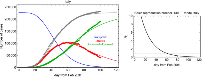
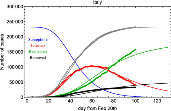
In order to solve the system in Eq. (1), while minimizing Eq. (3), we exploit numerical methods [12, 13]. In Fig. 1 (left), we show the result of the global fit for Italian data over 100 days. It turns out that $1/{\beta }_0\sim 1.8$ days and $1/\gamma \sim$ 32 days, and $R_0(0)=18$. The GoF is calculated to be of the order of 0.7 and 0.9 with the KS and R2 test, respectively. Therefore, the fit reproduces well the time dependence including lockdown effects (see discontinuity in the last period). $R_0$ as a function of time is shown in Fig. 1 (right). Errors on the fit parameters are very small and are not reported here because we believe they are not significant due to unknown uncertainties introduced by lockdown procedures and administration of medical tests. Yet, in Fig. 2 we show an error band taking into account three standard deviations determined from the fit residuals. From this figure, we can deduce: $1/{\beta }_0=1.8\pm 0.1$ days and $1/\gamma =32\pm 1$ days.

Fig. 1.

Left: Global fit of I (infected) and R (recovered+deceased) categories for Italian data since 20 February 2020. Right: $R_0(t)$ in the SIR-T model for Italian data

Fig. 2.

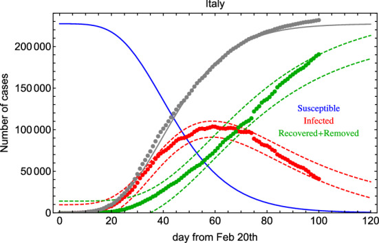
Global fit of I (infected) and R (recovered+deceased) categories for Italian data reporting error bands. See text for details

In Fig. 3, we show the daily new and recovered+deceased cases calculated from $\dot{I}+\dot{R}$ and $\dot{R}$, respectively. The SIR-T adopted model reproduces well the time dependence of the data. This is not the case at the same statistical significance level for the SIRD-T model in Eq. (4). In Fig. 4, we show the fit result for SIRD-T. As it is shown, the D and R categories are not described properly although the I category is described better. The KL (R2) GoF turns out to be 0.6(0.9) for the category recovered and deceased. The category of infected is well described by the model. For this fit, it turns out that $1/{\beta }_0\sim$ 1.8 days, $1/{\gamma }_R\sim$ 41 days, $1/{\gamma }_D\sim$ 145 days, and $R_0(0)=17.3$. We notice that $1/{\beta }_0$ and $R_0(0)$ are similar to the SIR-T case.

Fig. 3.

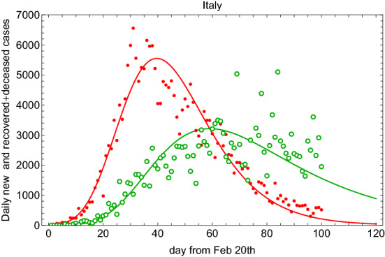
Fit to the daily new and recovered+deceased cases calculated from using $\dot{I}+\dot{R}$ (filled circle points) and $\dot{R}$ (open circle points) for Italian data since 20 February

Fig. 4.

Fit with the SIRD-T model for Italian data since 20 February 2020

The poorer description of the SIRD-T model is basically due to the fact the sum $D(t)+R(t)$ (simply called R(t) in the SIR-T model) is way more stable than the single compartments D(t) and R(t). This is clearly visible by comparing data from different countries, especially at the beginning of the pandemic spread, before the healthcare system reaches a stable regime in classification and treatments of different symptomatologies.

The $D(t)/(R(t)+D(t))$ ratio tends to the final so-called fatality rate, known with high accuracy only after the epidemic fade-out. As visible from [6], this ratio becomes smaller and smaller as the epidemic is close to the end in a specific country or region, as, for example, in China and South Korea, and/or in countries where the healthcare system intervention is approached with a more solid strategy, as, for example, in Germany.

For the reasons discussed above, we can conclude that SIRD-T can improve the understanding of the epidemic spread, as compared with SIR-T, only if R(t) and D(t) show smooth diverging rates and the fatality rate decreases monotonically. In this case, the different ${\gamma }_{R,D}$’s give a more accurate understanding of the hidden transfer functions between I(t) and R(t), or D(t).

Analysis of the German data

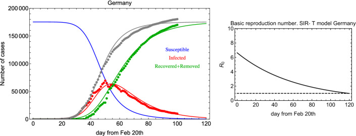
In order to compare the results above with the COVID-19 outbreak in other countries, we take into account data from Germany [6]. In Fig. 5 (left) and Fig. 5 (right), we show the fit result for the SIR-T model and $R_0$ as a function of time. For the Germany SIR-T model, it turns out that $1/{\beta }_0\sim$ 2.2 days, $1/\gamma \sim$ 15 days, and $R_0(0)=6.6$. So, in spite of the fact that the same model works well for both sets of data, the parameters are similar (same order) but not equal within the fit errors. This could be due to the different lockdown procedure, response, and health treatment. At the same time, it could indicate the limited accuracy of such a model to attempt to describe the same phenomenon in different frameworks. In Fig. 6, we show the daily new and recovered+deceased cases for Germany. In comparison with Fig. 3, the rate of change for recovered+deceased is clearly higher.

Fig. 5.

Left: Global fit of I (infected) and R (recovered+deceased) categories for Germany data since 20 February 2020. Right: $R_0(t)$ in the SIR-T model for Germany data

Fig. 6.

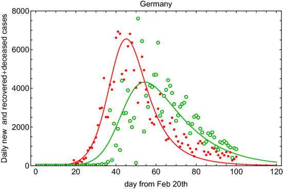
Fit to the daily new and recovered+deceased cases using $\dot{I}+\dot{R}$ (filled circle points) and $\dot{R}$ (open circle points) for Germany data since 20 February 2020

Accounting for asymptomatic cases: The SIAR-T Model

In this section, we account for asymptomatic cases in the basic SIR model. The set of equations are modified as follows:

$$\begin{array}{c}\hfill \begin{array}{cc}\hfill \frac{\mathrm{d}S(t)}{\mathrm{d}t}& =-{\beta }_S(t)\frac{S(t)I_S(t)}{N}-{\beta }_A\frac{S(t)I_A(t)}{N}\hfill \\ \hfill \frac{\mathrm{d}{I}_S(t)}{\mathrm{d}t}& ={\beta }_S(t)\frac{S(t)I_S(t)}{N}-{\gamma }_{S}I(t)\hfill \\ \hfill \frac{\mathrm{d}{I}_A(t)}{\mathrm{d}t}& ={\beta }_A\frac{S(t)I_A(t)}{N}-{\gamma }_{A}I(t)\hfill \\ \hfill \frac{\mathrm{d}R(t)}{\mathrm{d}t}& ={\gamma }_S{I}_S(t)+{\gamma }_A{I}_A(t)\hfill \\ \hfill \end{array}\end{array}$$ 7

where $I_A$ accounts for the asymptomatic population and ${\beta }_S(t)={\beta }_0{e}^{-\omega t}$. In this model to account for the lockdown effect, we assume as above a transmission rate for symtomatics changing with time. On the contrary, we assume a transmission rate constant in time for undetected asymptomatics. Assuming an early exponential growth for both $I_S$ and $I_A$, we obtain the constraint: ${\beta }_S>{\beta }_A$ and ${\gamma }_S>{\gamma }_A$. The fit has seven free parameters, namely $\widehat{\theta }=\{{\beta }_S,{\beta }_A,{\gamma }_S,{\gamma }_A,N,I_S(0),I_A(0),\omega \}$. In Fig. 7, we show the result of the fit for data from Italy.

Fig. 7.

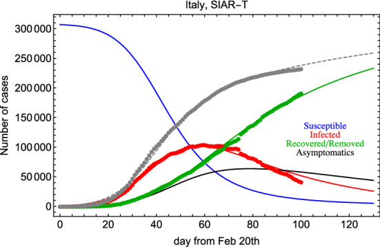
Fit to Italian data with the SIAR-T model

The KL(R2) GoF is equal to 0.92(0.89) for the infected category and practically 1 for the recovered/removed category. In addition, $1/{\beta }_0\sim$ 5.0 days, $1/{\beta }_A\sim$ 7.0 days, $1/{\gamma }_S\sim$ 41.0 days, $1/{\gamma }_A\sim$ 78.0, and $R_0={\beta }_0/{\gamma }_S\sim$ 8.2. We notice that the asymptomatic population could play an important role and it is characterized by a longer transmission time. This latter point may be due to the fact that asymptomatics have a poorer infection “power”.

The daily cases for this SIAR-T model are shown in Fig. 8.

Fig. 8.

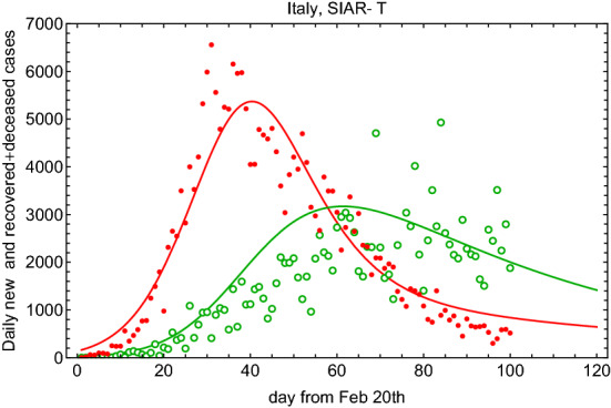
Fit to the daily new and recovered+deceased cases using $\dot{I}+\dot{R}$ (filled circle points) and $\dot{R}$ (open circle points) for the SIAR-T model and for Italy data since 20 February 2020

We notice, however, that the model described in (7) is sensitive only to a non-constant ratio $I_S(t)/I_A(t)$. If asymptomatic cases are a constant fraction of the visible cases, the model could not be able to detect any anomaly in the observable compartments. As a consequence, the $I_A(t)$ must be interpreted as a possible deviation from the constant ratio. It is interesting to notice that the unknown fraction of asymptomatic cases does not invalid the SIR model and its modifications as it is proposed in this work. This hidden component changes of course the interpretation of $R_0$ and of other parameters that are referred to the observables.

Conclusions

In this work, we proposed time-dependent modifications of the SIR compartmental model, referred to as SIR-T, SIRD-T, and SIAR-T, as fit models for understanding the evolution of the COVID-19 outbreaks in Italy and Germany during the lockdown. In particular, those models allow us to infer the most important epidemic parameters fitting simultaneously active and concluded cases in the presence of lockdown and social distancing restrictions.

The study that we have reported in this paper shows that the SIR model, with the changes proposed above, describes so far satisfactorily the COVID-19 Italian data time dependence with lockdown effects. The same model and assumptions work for other country data, as, for example, for Germany. Yet, in some cases reported, as an example, for the latest Spanish data, South Korean data, and Chinese data [6] some non-statistical effects are evident. These effects can be due to a strong lockdown procedure impact or to a sudden increase of the infection. In these cases, the statistical model discussed in this work is not appropriate to account for important discontinuities in the data. However, it is worth mentioning that indeed the effect of the lockdown is evident in the data that we have analysed. As a matter of fact, data show small discontinuities due to the lockdown which, at this level, are taken care by the model described in present work.

Among all candidates, the SIR-T model represents, given its simplicity, the best model fit, being the concluded cases (recovered+deceased) more stable with respect to the separate components, even in the presence of an asymptomatic hidden component (especially if in constant ratio with the visible components). This model represents a good candidate for predicting the time evolution of the outbreak, with a sizable time scale, especially after the active case peak is overtaken.

The model has satisfactory agreement with data if restrictions play important role in limiting the possible susceptible population inside the virtual box. If restrictions are reasonably respected, the model predicts the end of the critical period in less than a few months. Yet, the model seems not sensitive to the asymptomatic category, which can play an important role. Inattention and carelessness by communities and governments will open the virtual box again exposing more people to the infection and creating a new starting point for the new cases evolution. In cases of lack of attention to the lockdown, the model fails to predict the evolution because of out-of-control effects.

References

- 1.https://www.who.int/health-topics/coronavirus/
- 2.Neeltje van Doremalen et al. Aerosol and surface stability of HCoV-19 (SARS-CoV-2) compared to SARS-CoV-1. The New England Journal of Medicine, 10.1056/NEJMc2004973. [DOI] [PMC free article] [PubMed]
- 3.E. Lavezzo et al. Suppression of COVID -19 outbreak in the municipality of Vo, Italy. 10.1101/2020.04.17.20053157
- 4.Kermack WO, McKendrick AG. Royal Soc. London Proc. Ser. A. 1927;115:700–721. [Google Scholar]
- 5.Chen Yi-Cheng, et al. Access IEEE. 2020;8:164012–164034. doi: 10.1109/ACCESS.2020.3021952. [DOI] [PMC free article] [PubMed] [Google Scholar]
- 6.https://www.worldometers.info/coronavirus/
- 7.James F, Roos M. Minuit: A System for Function Minimization and Analysis of the Parameter Errors and Correlations. Comput. Phys. Commun. 1975;10:343–367. doi: 10.1016/0010-4655(75)90039-9. [DOI] [Google Scholar]
- 8.Smirnov N. Ann. Math. Stat. 1948;19(2):279–281. doi: 10.1214/aoms/1177730256. [DOI] [Google Scholar]
- 9.Roe BP. Probability and Statistics in Experimental Physics. New York: Springer-Verlag; 2001. [Google Scholar]
- 10.Steel RGD, Torrie JH. Principles and Procedures of Statistics with Special Reference to the Biological Sciences. New York: McGraw Hill; 1960. [Google Scholar]
- 11.https://covid19.infn.it/
- 12.Runge C. Ueber die numerische Auflsung von Differentialgleichungen. Math. Ann. 1895;46:167–178. doi: 10.1007/BF01446807. [DOI] [Google Scholar]
- 13.Kutta W. Beitrag zur naherungsweisen Integration von Differentialgleichungen. Z. Math. Phys. 1901;46:435–453. [Google Scholar]