Improving the prediction accuracy of protein abundance in Escherichia coli using mRNA accessibility

Abstract

RNA secondary structure around translation initiation sites strongly affects the abundance of expressed proteins in Escherichia coli. However, detailed secondary structural features governing protein abundance remain elusive. Recent advances in high-throughput DNA synthesis and experimental systems enable us to obtain large amounts of data. Here, we evaluated six types of structural features using two large-scale datasets. We found that accessibility, which is the probability that a given region around the start codon has no base-paired nucleotides, showed the highest correlation with protein abundance in both datasets. Accessibility showed a significantly higher correlation (Spearman’s ρ = 0.709) than the widely used minimum free energy (0.554) in one of the datasets. Interestingly, accessibility showed the highest correlation only when it was calculated by a log-linear model, indicating that the RNA structural model and how to utilize it are important. Furthermore, by combining the accessibility and activity of the Shine-Dalgarno sequence, we devised a method for predicting protein abundance more accurately than existing methods. We inferred that the log-linear model has a broader probabilistic distribution than the widely used Turner energy model, which contributed to more accurate quantification of ribosome accessibility to translation initiation sites.

INTRODUCTION

In the first step of prokaryotic translation, a ribosome binds to the Shine–Dalgarno (SD) sequence immediately upstream of the start codon (1,2). RNA secondary structure around the SD sequence hinders the access of the ribosome and reduces the efficiency of translation (3). The inhibitory effect of secondary structure spreads downstream of the start codon, according to protein abundance data derived from more than 100 synthetic mRNAs encoding the same green fluorescent protein (GFP) (4). Specifically, the correlation between protein abundance and predicted free energy of RNA folding is the highest when the region for calculating free energy includes greater than 30 nucleotides (nt) located downstream from the start codon (4). The predicted free energy for the region downstream of the start codon is one of the most useful features explaining protein abundance based on data obtained from extensive DNA synthesis and protein measurements (5).

Recent advances in high-throughput DNA synthesis have enabled us to synthesize tens of thousands of short (∼230 nt) DNAs simultaneously at a low cost (6). Two recent studies used this technique to generate large amounts of protein abundance data for various synthetic mRNA sequences encoding GFP (7,8). Although the number of synthetic sequences for which protein abundance was measured by a single study has drastically increased from 154 to 244 000 in the last decade (4,8), bioinformatics techniques to evaluate secondary structural features have not made full use of those data. Previous studies used the minimum or ensemble free energy calculated around the start codon to investigate the relationship between secondary structure and large-scale protein abundance data (4,5,7,8). As shown in these studies, as well as in the present study, only a medium correlation is observed between protein abundance and free energy. Therefore, there may be other structural features that could be used to explain protein abundance more accurately.

Minimum and ensemble free energies are used widely to predict the existence of RNA secondary structures. These free energies are calculated based on the Turner energy model (9,10). The Turner energy model has long been used for a wide variety of analyses related to RNA secondary structure. The software tools implementing this model are maintained well (11,12). Thus, one can easily use this model to calculate various types of secondary structural features. Although the Turner energy model is currently used as the de facto standard, there are other types of models, such as probabilistic models constructed using a data-driven approach. Do et al. developed a conditional log-linear model for predicting RNA secondary structure. This model has a similar set of parameters as the Turner model, but its values are optimized such that the probability of the verified secondary structure is maximized (13). Although the authors showed that their model achieved better accuracy in the prediction of secondary structure of small non-coding RNAs, it has not been used to infer protein abundance from mRNA sequences. Hereafter, we describe their model as the CONTRAfold model.

There is another line of research that aims to predict protein abundance based on the SD sequence and RNA secondary structure. RBSDesigner (14), RBSCalculator (15), and UTR Designer (16) have been proposed for this purpose. In these tools, structural features other than free energy are used, including the interaction free energy between rRNA and mRNA, exposure probability of ribosome binding sites, and secondary structure of the so-called ‘stand-by’ site. These structural features are calculated by the Turner energy model.

In the present study, we used two large-scale protein abundance datasets to identify useful secondary structural features. We calculated different secondary structural features using the Turner and CONTRAfold models and evaluated their correlation with protein abundance. Overall, the features calculated by the CONTRAfold model showed comparable or better correlations than those calculated by the Turner model. Accessibility, which is the probability that a given region around the start codon has no base-paired nucleotides, showed the highest performance when it was calculated by the CONTRAfold model. As indicated later, the probabilistic distribution of the CONTRAfold model should be broader than that of the Turner energy model, which may contribute to a more accurate prediction of ribosome accessibility to translation initiation sites where RNA secondary structure must be transiently unwound at the moment of translation initiation.

MATERIALS AND METHODS

Secondary structural features

We evaluated six types of secondary structural features:

• accT: accessibility calculated by the Turner model

• accC: accessibility calculated by the CONTRAfold model

• mfeT: minimum free energy calculated by the Turner model

• mfeC: Viterbi score calculated by the CONTRAfold model

• ensT: ensemble free energy calculated by the Turner model

• ensC: inside-outside score calculated by the CONTRAfold model

We calculated these secondary structural features at various regions around the start codon. Suppose that r is a region around the start codon, accessibility is defined as the probability that no base in r forms a base pair in the mRNA sequence x (17,18).

(1)

where Ω_r is a set of secondary structures that have no base pairs in r, and P(σ|x) is the probability of the RNA sequence x forming the structure σ. The definition of P(σ|x) differs depending on the model used; in the Turner energy model, it is defined based on the Boltzmann distribution, while in the CONTRAfold model, it is defined by the log-linear function. In either case, −RTlnP(r|x) is interpreted as the free energy needed to remove all base pairs from the region, where R and T are the gas constant and temperature, respectively. In this study, we used the transformed accessibilities as accT and accC. The region r can be a single nucleotide, and in that case, accC and accT represent position-specific accessibility. Accessibility including position-specific one has also been used for the analyses of target sites of microRNA (19,20) and bacterial sRNA (21).

The minimum free energy (mfeT) and ensemble free energy (ensT) are widely used measures to evaluate the stability of RNA secondary structure, and are calculated based on the Turner energy model. mfeC and ensC are analogs of mfeT and ensT, respectively, calculated based on the CONTRAfold model. While mfeT (mfeC) considers the single most probable structure, ensT (ensC) considers all possible structures. Lower free energy calculated by the Turner model indicates the existence of more stable secondary structures. Conversely, a lower score obtained with the CONTRAfold model indicates the presence of more unstable secondary structures. To avoid this discrepancy, we multiplied the Viterbi and inside-outside scores by –1 and used them as mfeC and ensC, respectively.

Intuitively, the difference between accessibility and minimum (or ensemble) free energy is the base pairs that are taken into account. Suppose that we calculate the accessibility and minimum free energy of the same region r in an mRNA sequence. The former considers all base pairs in the mRNA sequence, and the latter only considers base pairs within r, as illustrated in Figure 1.

Figure 1.

Differences of the base pairs that are taken into account. For a given region r in an mRNA, accessibility considers all base pairs, while the minimum and ensemble free energies consider the base pairs written in black.

We used the Raccess program (18) to calculate accT and accC, ViennaRNA package version 2.1.9 (11) to calculate mfeT and ensT, and CONTRAfold program version 2.01 (13) to calculate mfeC and ensC.

Similarity and difference between the Turner and CONTRAfold model

The two models have similar sets of parameters and calculate the contribution of secondary structural component, such as hairpin, bulge, internal, multi loop, and two consecutive base pairs, based on the parameters. The sum of the contributions represents the free energy (or score in the CONTRAfold model) of the whole secondary structure. In principle, the same types of calculation related to secondary structure can be done by either models. For example, we can calculate the most probable secondary structure and base-pair probabilities for a given sequence by either models.

The important difference between the Turner and CONTRAfold model is parameter values they employed. The former uses the parameter values determined by thermodynamic experiments, while the latter uses those values obtained by a machine learning approach, in which parameter values are optimized such that the probability of known secondary structure in training data is maximized. For example, in the Turner model, the contribution of two consecutive base pairs, A–U followed by G–C, is determined by a single parameter value of –2.4 kcal/mol. In the CONTRAfold mode, it is calculated as the sum of three parameter values; parameter values for A–U pair, G–C pair, and stacking of A–U on G–C are 0.6, 1.54 and 0.56, respectively. Therefore, the contribution of A-U followed by G–C is 2.7 (= 0.6 + 1.54 + 0.56) arbitrary unit.

mRNA sequences and protein abundance data

We used three datasets to investigate the relationship between RNA secondary structure and protein abundance.

• Dataset 1 consisted of 244 000 mRNA sequences and their corresponding protein abundance values measured by Cambary et al. (8). These mRNAs have the same 5′-untranslated region (UTR) and different sequences in their N-terminus codons. We used 120-nt mRNA sequences surrounding the start codon to calculate secondary structural features, including 30 nt upstream and 90 nt downstream of the start codon. The authors used at most 30 nt upstream of the start codon to investigate secondary structural features (8). We also assumed that 90 nt downstream of the start codon are important for evaluating structural features around the start codon. The length of 120-nt mRNA should be reasonable in that long-range base pairs in mRNAs, which were shown to be less accurately predicted (22), are not included. We used the P_NI value as the protein abundance value, which quantified protein production under normal conditions in which RNA secondary structure around the start codon was not manipulated artificially.

• Dataset 2 consisted of a large part of the data obtained by Goodman et al. (7). They measured the protein abundance of mRNA sequences transcribed from different promoters. These mRNAs not only have different sequences in their N-terminus codons but also possess different 5′-UTRs. Dataset 2 consisted of protein abundance values and corresponding mRNA sequences that possess three different 5′-UTRs containing ribosome binding sites of varying strength. To cancel the effects of different 5′-UTR sequences and being transcribed from different promoters, we divided the dataset into 6 groups such that the mRNAs in each group had the same UTR and were transcribed from the same promoter. Each of the six groups consisted of approximately 1770 mRNAs and their corresponding protein abundance values. We used mRNA sequences starting from the transcription start sites and ending at 90 nt downstream of the start codon to calculate the secondary structural features. We used log-transformed protein scores provided by (7) as the protein abundance values.

• Dataset 3 is derived from the remaining part of the data obtained by Goodman et al. (7). It contained 1733 protein abundance values and corresponding mRNA sequences with 137 different endogenous 5′-UTRs. These mRNAs were transcribed from strong promoter. An important difference between Datasets 3 and 2 is that the mRNAs in the former dataset have many different 5′-UTR sequences. We used this dataset to combine the effects of the SD sequence and RNA secondary structures. We classified this dataset into 137 groups based on the UTR sequences. In the sequence design by Goodman et al., mRNAs with the same endogenous 5′-UTR encode the same amino acid residues in their N-terminus codons. As a result, the mRNAs in each group consisted of approximately 13 distinct sequences that possessed the same UTR and encoded the same amino acids. This classification was used to train and test the predictive models based on the SD sequence and structural features. The definitions of mRNA sequences used for calculating secondary structural features and protein abundance values were the same as those of Dataset 2.

Machine learning algorithms

We used a machine learning approach for two purposes. The first was to construct predictive models based on position-specific structural features. For this, we used the random forest regression implemented in the ranger package of the R statistical computing environment (version 3.5.2). Random forest regression is an algorithm for predicting a real-valued ‘target’ variable based on multiple regression trees, each of which is trained from a subset of training data. It not only handles non-linear relationship between the target variable and features in training data, but also can be used to calculate the importance of features. It has been used to analyze high-dimensional data from the life sciences such as gene expression and genome-wide association studies (23). The ranger function was run using the default parameters. To estimate the importance of position-specific features, we calculated the corrected impurity importance measure proposed by (23), which was also implemented in the ranger package. Roughly speaking, the importance measure represents the mean decrease of the sum of square error between predicted and true value when a particular feature is taken into account during the construction of regression trees.

The second purpose was to integrate the effects of the SD sequences and RNA secondary structures. We evaluated three types of regression algorithms using Dataset 3. Linear, random forest, and support vector regressions were used with the lm function, the ranger package, and e1071 package in the R statistical computing environment (version 3.5.2), respectively. All of the algorithms were run with the default parameters, and hence the RBF kernel was used for support vector regression.

Cross validation

We used Dataset 1 to train and test the predictive models based on position-specific features. Some mRNA sequences in this dataset were quite similar to one another. To avoid overfitting to the mRNAs and to ensure fair validation, care must be taken in determining the training and test data. In this dataset, the nucleotide sequences of the mRNAs had been computationally designed by iterative mutations of the 57 seed sequences (8). The mRNA sequences derived from the same seed sequence were similar to one another. Therefore, we used mRNA sequences derived from one seed sequence as test data, while those derived from the remaining seed sequences were used as training data.

We used Dataset 3 to integrate the effects of the SD sequence and RNA secondary structures. As described above, we classified this dataset into 137 groups, and the mRNA sequences in each group were similar because they had the same UTR and encoded the same amino acids. We used the mRNA sequences in one group as test data and those in the remaining group as training data.

Measurement of prediction accuracy

We mainly used Spearman’s rank correlation coefficient (ρ) values to evaluate not only secondary structural features but also existing tools, because they do not always show linear correlations with protein abundance. The units and measurable range of protein abundance values were different across experimental systems. Furthermore, the scores of existing tools were not intended to reflect the protein abundance values derived from a specific experimental system. Therefore, we used Spearman’s ρ rather than Pearson’s correlation coefficient (R).

RESULTS

Correlation between secondary structural features and protein abundance in Dataset 1

First, we evaluated the six secondary structural features using Dataset 1. We calculated the secondary structural features at various regions around the start codon and compared them with protein abundance. As an example, Figure 2 shows Spearman’s ρ values between accC and protein abundance, calculated at various regions. The same heatmap for the other features is shown in Supplementary Figure S1. In the case of accC, the maximum correlation was observed when the region was from -19 to +15, where the first nucleotide of the start codon was set to be 0. Hereafter, we denote the region showing the highest correlation as the optimal region. Table 1 shows Spearman’s ρ values for each of the six structural features calculated at the optimal region. Overall, the features calculated by the CONTRAfold model performed better than those produced by the Turner model in this dataset, and accC showed the highest correlation. It is notable that the ρ values are different among the three features calculated by the CONTRAfold model. For example, there was a 7.7% difference between the ρ value of accC and that of ensC, which was the second highest feature. This indicates that the model and type of structural feature are both important for achieving a higher correlation. It should also be noted that accC showed significantly higher correlations than the widely used mfeT. Figure 3 shows a 2D plot of these two structural features against 10 000 randomly selected protein abundance values. As can be seen in this figure, the relationship between mfeT and protein abundance is more scattered than that of accC.

Figure 2.

Spearman’s ρ values between accC and protein abundance. The X-axis represents the center position of a region used for calculating accC. The Y-axis represents the length of the region. Position 0 indicates the first position of the start codon. The ρ value was largest when the region was from –19 to +15. The ρ values at the regions protruding outside the mRNA sequences cannot be calculated and are shown in black.

Table 1.

Maximum correlation for the six structural features

Feature	Spearman’s ρ value	Optimal regiona	Lengtha (nt)
accT	0.575	−17:+17	35
accC	0.709	−19:+15	35
mfeT	0.554	−30:+41	72
mfeC	0.605	−30:+41	72
ensT	0.561	−30:+40	71
ensC	0.632	−30:+41	71

^aThe region and its length at which the maximum ρ value is observed.

Figure 3.

Two-dimensional plot between protein abundance and secondary structural features. mfeT is the minimum fee energy; accC is accessibility calculated by the CONTRAfold model. a.u. = arbitrary unit.

The length of the optimal region for accC was 35 nt, which is slightly longer than the length protected by the ribosome (28 nt) in ribosome profiling experiments (24). It was reported that secondary structures up to +13 strongly reduce protein abundance (25), which was consistent with the optimal region for accC. As shown in the last column of Table 1, the lengths of the optimal region are shorter for accT and accC than for the other structural features. Effective accessibility was influenced by base pairs not only within the optimal region but also in the outside regions, as illustrated in Figure 1.

Next, we calculated Spearman’s ρ among the six features (Figure 4). The minimum and ensemble free energies including their analogs, that is, mfeT, mfeC, ensT, and ensC, were similar to each other. There was a high correlation between accT and accC, although the latter showed a significantly higher correlation with protein abundance than the former. The three features calculated by the Turner model, that is, accT, mfeT and ensT, showed comparable correlations with protein abundance (Table 1), but the correlations between accT and mfeT, and between accT and ensT, were low. When we used Pearson’s R instead of Spearman’s ρ, we obtained almost the same result (Supplementary Figure S2).

Figure 4.

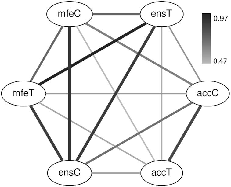
Spearman’s ρ values among the six structural features. The darkness of the edges indicates the ρ value. In addition, the width of the edges is proportional to the ρ value for readability.

We also evaluated two existing tools, RBSDesigner and RBSCalculator, to predict protein abundance. Spearman’s ρ values between protein abundance and the scores of RBSDesigner and RBSCalculator (version 1.0) were 0.440 and 0.540, respectively. Thus, the performance of these tools was comparable or lower than that of the six features, although these tools take into account several different structural features. UTR Designer and the newer version of RBSDesigner (version 2.0 or later) were not evaluated here because they are web-based tools and could not be used to evaluate a large number of mRNAs.

Predictive model based on position-specific accessibility

We investigated whether more detailed secondary structural features were useful for predicting protein abundance. Specifically, having observed that accC showed the best performance, we calculated accC in each position from –30 to +89 and used them as the features for training predictive models. We converted each mRNA sequence into a 121D vector consisting of accC in each position as well as accC at the optimal region. The vectors and corresponding protein abundance values were used to train a random forest regression model. In the cross validation described in the Methods, Spearman’s ρ value was 0.758, indicating that considering the accC at each position increased the correlation by 4.9%. When we calculated the importance of features by the random forest model, we observed that the most important feature was accC at the optimal region, as expected. In addition, accC in each position showed various degrees of importance. Figure 5 shows the importance of accC in each position. The positions with the top 6 highest importance were within the plausible SD sequence, indicating that the accessibility of the SD sequence was more important than that of the other positions. Positions +30 and higher showed little contribution to prediction accuracy. Actually, when we excluded accC in these positions from the feature vector, we observed almost the same, slightly higher ρ values in the same cross validation, suggesting that the nucleotides in these positions rarely participated in the formation of base pairs that disturbed the access of the ribosome.

Figure 5.

Importance of accessibility in each position. The position and nucleotides of a plausible SD sequence are indicated in the yellow box and letters above the box, respectively. a.u. = arbitrary unit.

Evaluation of the secondary structural features by Dataset 2

Next, we evaluated the six structural features using Dataset 2. As described above, the mRNAs were transcribed from two different promoters and had three types of UTRs. To cancel the effect of different UTRs and the strength of the promoters, we divided this dataset into six groups and evaluated the structural features for each group separately. Table 2 shows the Spearman’s ρ values for the six structural features at the optimal region. accC showed the highest correlation in all but one group, denoted by LW. In this group, mRNAs were transcribed from a low-activity promoter and had a 5′-UTR with a weak ribosome binding site, and 96% of the protein abundance values in this group were below the detection limit according to (7). Therefore, the protein abundance data in this group may not be reliable. Actually, the ρ values of this group were at most 0.445, which was much lower than those of the other groups. Therefore, we concluded that accC was better than the other structural features in Dataset 2, as was the case in Dataset 1.

Table 2.

Evaluation of the structural features in each group of Dataset 2

	Spearman’s ρ						Optimal region
Feature	HW	HM	HS	LW	LM	LS	HW	HM	HS	LW	LM	LS	Ave. len.a
accT	0.693	0.641	0.552	0.394	0.635	0.658	+5:+64	+2:+20	−12:+20	−25:+36	−22:+72	−25:+21	52.7 ± 26.4
accC	0.787	0.738	0.611	0.440	0.746	0.753	−13:+19	−18:+18	−18:+15	−25:+29	−22:+20	−25:+18	41.0 ± 8.2
mfeT	0.728	0.642	0.536	0.420	0.654	0.648	−22:+56	−20:+56	−18:+56	−24:+56	−22:+59	−22:+56	78.8 ± 2.6
mfeC	0.632	0.573	0.492	0.353	0.558	0.579	−23:+66	−18:+65	−16:+66	−25:+67	−23:+65	−26:+66	88.7 ± 4.3
ensT	0.747	0.658	0.550	0.428	0.668	0.663	−21:+56	−17:+56	−17:+56	−25:+56	−23:+56	−22:+56	77.8 ± 3.3
ensC	0.754	0.665	0.560	0.445	0.681	0.681	−23:+65	−21:+65	−25:+57	−25:+67	−22:+65	−26:+66	88.8 ± 3.8
accCopt1 b	0.767	0.736	0.610	0.404	0.736	0.746	–	–	–	–	–	–	–
RFopt1 c	0.703	0.645	0.539	0.372	0.621	0.610	–	–	–	–	–	–	–
RBSDesigner	0.597	0.561	0.441	0.300	0.539	0.534	–	–	–	–	–	–	–
RBSCalculator	0.631	0.569	0.476	0.300	0.595	0.594	–	–	–	–	–	–	–

HW, HM, HS, LW, LM, and LS are the group codes. The first and second letters of the code indicate the type of promoter and 5′-UTR, respectively (H: high, L: low promoter; S: strong, M: middle, W: weak UTR). The highest ρ value in each group is written in bold.

^aThe average length of the optimal region (± standard deviation)

^baccC calculated at the optimal region in Dataset 1, that is, −19:+15

^cRandom forest regression model trained using Dataset 1

As with Dataset 1, the lengths of the optimal region of accT and accC were shorter than those of the other features (Table 2, last column). When we focused on accT and accC, the variation of the length of the optimal region across the groups was found to be smaller in accC than in accT. Therefore, accC was more stable than accT in terms of the length variation of the optimal region.

We also evaluated the accuracy of accC calculated at the optimum region in Dataset 1 (–19:+15) ( in Table 2). It showed a comparable correlation with accC in Dataset 2, indicating that the difference of the optimal region of accC between Datasets 1 and 2 had little influence on the prediction accuracy. However, when we evaluated the random forest regression model trained by Dataset 1 ( in Table 2), it showed a lower correlation than accC and was sometimes beaten by the other structural features. We speculated that the lower correlation of was due to inherent biases caused by a particular experimental system and/or the so-called ‘batch effect’ in these large-scale datasets, which is discussed in more detail later. We also evaluated the accuracy of RBSDesigner and RBSCalculator version 1.0 (Table 2); they showed comparable or lower correlations than the six structural features, as in Dataset 1.

We next investigated the importance of position-specific accC. For each group, we used the random forest regression model to calculate the importance values of position-specific accC, as described in the analysis of Dataset 1. Due to the length differences of mRNAs in Dataset 2, the method for constructing the feature vectors was slightly different from the case of Dataset 1 (see Supplemental material). Figure 6 shows the importance values of a position-specific accC in Dataset 2. Note that the scale of the Y axis of Figure 6 varies depending on the group. This is because the importance measure proposed by (23) is the mean decrease of the sum of square error when a particular feature is taken into account, and its scale varies depending on the data for calculating it. Similar to Dataset 1, the importance values immediately downstream of the start codon tended to be high in all groups. However, the positions around potential SD sequences showed variable importance depending on the groups. Compared to the importance values immediately downstream of the start codon, those values around the SD sequences were lower in HM and HS than in the other four groups, suggesting that the importance of accessibility around the SD sequence differed depending on the activity of the SD sequence and strength of the promoter.

Figure 6.

Importance of the accessibility of each position in Dataset 2. HW, HM, HS, LW, LM and LS are the group codes. The first and second letters of the code indicate the type of promoter and 5′-UTR, respectively (H: high, L: low promoter; S: strong, M: middle, W: weak UTR). The position and nucleotides of plausible SD sequences are indicated by the yellow box and letters above the box, respectively. a.u. = arbitrary unit.

Combining SD sequence and accessibility

Translation initiation is affected by the SD sequence and RNA secondary structure. For example, the ribosome binds strongly to the SD sequence of AGGAGG, which is complementary to the 3′-end of rRNA. There are several tools for predicting protein abundance considering the SD sequence and RNA secondary structure, such as RBSDesigner, RBSCalculator and UTR Designer. Here, we tried to create a more accurate method by combining accC and the SD sequence. For this purpose, we used Dataset 3, which was a part of the data measured by Goodman et al. To our knowledge, this is the only large-scale dataset in which many different SD sequences and variable secondary structures around the start codon are investigated simultaneously. To infer the strength of the SD sequence, we used the EMOPEC program developed by Bonde et al. (26). The authors experimentally measured the activity of all possible SD sequences and developed the EMOPEC program to predict the activity of SD sequences without considering secondary structure. Figure 7A shows the relationship between accC, the EMOPEC score, and protein abundance in Dataset 3. Here, we used accC calculated at the optimal region in Dataset 1 (–19:+15). When accC was less than –4, the protein abundance values tended to be low, even when the EMOPEC score was high, that is, when the mRNAs have strong SD sequences. When accC was greater than –3, the protein abundance values depended on the EMOPEC score. Thus, it is clear that both features affected protein abundance. We used accC and the EMOPEC score to train predictive models using three different machine learning algorithms, namely, linear, random forest, and support vector machine (SVM) regression. We found that prediction accuracy did not vary greatly among these three algorithms. Figure 7B shows correlation coefficients between the observed and predicted protein abundance values based on the cross validation described in the Methods. Spearman’s ρ was the highest when linear regression was used, although Pearson’s R was the highest when SVM was used. We decided to use linear regression, because it is the simplest model and is unlikely to have a problem of overfitting.

Figure 7.

Evaluation of predictive models using Dataset 3. (A) Two-dimensional plot between the EMOPEC score and accC. Color represents the protein abundance value. (B) Comparison of the prediction accuracy of three machine learning algorithms.

Figure 8 shows the prediction accuracy of our method and existing methods. UTR Designer and RBSCalculator version 2.0 or later were not included, because they are web-based tools and could not be used to evaluate a large number of mRNAs. The EMOPEC score alone did not perform well, probably because it did not consider RNA secondary structures. However, when it was combined with accC using linear regression, it showed a higher correlation than the existing methods. Furthermore, we found that considering another start codon improved prediction accuracy. In Dataset 3, mRNAs have another potential start codon located 33 nt downstream from the canonical start codon. The open reading frame starting from the second ATG encoded complete GFP (7). The second ATG could also contribute to protein abundance, because the mRNAs in this dataset had variable sequences between the two ATGs and it is possible that there was accidentally a strong SD sequence located immediately upstream of the second ATG. We inferred protein abundance values for the two ATGs (denoted by p1 and p2) and combined them by ln(exp(p1) + exp(p2)), because the protein abundance values were log transformed. When we used the combined values as a prediction of protein abundance, we observed that the correlation coefficients were improved by ∼3.5% (the rightmost bar in Figure 8), suggesting that the second ATG contributed to protein abundance. We have implemented the linear regression-based predictive model as command-line software, which is available at GitHub (https://github.com/gterai/RBSeval).

Figure 8.

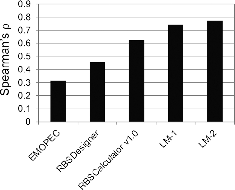
Comparison of our method and existing methods. LM-1 is a linear regression model based on the EMOPEC score and accC. LM-2 is the same linear regression model but considers two start codons (see text for details).

DISCUSSION

In this study, we evaluated six different secondary structural features and found that accC, which is accessibility calculated by the CONTRAfold model, showed the highest correlation with protein abundance. Furthermore, by combining accC and the inferred activity of the SD sequence, we created a method for predicting protein abundance that was more accurate than existing methods.

Why did accC perform better?

The secondary structure around the start codon must undergo conformational changes at the initiation of translation. At the moment when the ribosome accesses the mRNA, the RNA secondary structure should be unwound. We speculate that the CONTRAfold model is more appropriate for evaluating secondary structure having such conformational changes. The probabilistic distribution of the secondary structure in the CONTRAfold model should be broader than that of the Turner model.

As shown in Supplementary Figure S2, the minimum free energy (mfeT) and ensemble free energy (ensT) had an almost perfect correlation (ρ = 0.972); for the CONTRAfold model, mfeC and ensC were less similar (ρ = 0.891). This indicates that a single most probable secondary structure occupies a larger part of the whole distribution in the Turner model than in the CONTRAfold model. It is possible that the CONTRAfold model was able to detect the existence of a sub-optimal secondary structure, which contributed to a more accurate quantification of ribosomal access.

Furthermore, accessibility considers all possible base pairs in the input mRNA sequence, not only the ones within a region around the start codon, as illustrated in Figure 1. This may have a positive effect on detecting the base pairs that disturb ribosomal access.

Position-specific structural features did not improve the prediction accuracy

Recent advances in experimental systems allow us to measure protein abundance derived from a vast number of synthetic mRNAs (7,8). Dataset 1 contained data from as many as 244 000 synthetic mRNAs. It seemed possible that we were able to extract more detailed secondary structural features from this large-scale dataset. When we used the random forest model based on position-specific accC, prediction accuracy was increased (ρ = 0.758) in the cross-validation analysis using Dataset 1. Furthermore, we observed that the accessibility of the SD sequence was more important than that of the other positions (Figure 5), which was biologically reasonable. Indeed, the importance of secondary structure around the SD sequence has been shown by different experimental systems (27,28). However, we observed that the random forest model trained by Dataset 1 did not perform well in Dataset 2 (RF^opt1 in Table 2). As shown in Figures 5 and 6, the importance of accessibility around SD sequences was different between and within the datasets, which might explain the lower performance of . We also suspect that the random forest model constructed based on the position-specific features captured biases caused by a particular experimental system and/or the batch effect, which are commonly found in high-throughput experiments (29). No experimental system is perfect and may have specific biases. For example, in Dataset 2, the amino acids of the N-terminus region of GFP were different among the mRNA sequences, which can cause different translation elongation speeds and fluorescent intensity. In addition, high levels of protein expression can cause growth defects, which might lead to a decrease in the number of ribosomes in a cell. The random forest model trained by Dataset 1 may have captured such biases, which could have led to its reduced performance when applied to Dataset 2. This result showed the risk of using complex predictive models trained by a single dataset.

Future directions

There are two important directions to be explored. First, the usefulness of accC should be validated in other bacteria. Here, we used the data obtained in E. coli, because it is the only prokaryotic species for which large-scale datasets are available. In principle, accC is expected to be useful in other prokaryotes, because the mechanism of translation initiation is the same across prokaryotes. Previous studies have shown that the suppression of secondary structures around the start codon is a general feature of prokaryotes (30). However, it is possible that the optimal region for calculating accC might differ between bacteria. Furthermore, the importance of the SD sequence can vary in different bacteria. Therefore, tuning the region for calculating accC and the importance of SD sequences for each prokaryote may contribute to the precise prediction of protein abundance in other bacterial species, especially in gram-positive bacteria in which the importance of the SD would be much less important. It might be interesting to explore the possibility to evaluate secondary structural features using genomic data (such as ribosome profiling data). Indeed, we have been trying to evaluate secondary structural features using ribosome profiling data from not only Escherichia coli but also other bacteria. From this analysis, however, we observed that correlation coefficients between secondary structural feature and translation efficiency deduced from ribosome profiling data were much lower than those observed in the current study, even if the SD sequence was taken into account (data not shown). There are many possible causes of the low correlation coefficients, such as intrinsic gene regulation for endogeneous genes, noise in ribosome profiling data, translational re-initiation in closely located genes in an operon, and different codon usage bias in each gene. If these causes are elucidated and removed, it may be possible to use genomic data for the evaluation of secondary structural features.

The other direction is to consider the joint secondary structure between ribosomal RNA and mRNA. The binding of rRNA to the SD sequence may compete with the formation of secondary structure around the start codon. Therefore, in principle, we should consider the competition between them for predicting protein abundance. Existing tools, such as RBSCalculator, RBSDesigner, and UTR Designer, quantitatively evaluate this competition based on the Turner model. It is interesting that our simple linear regression model, which does not consider the joint structure, showed a higher prediction accuracy than the existing methods (Figure 8). This suggests that the competition between RNA secondary structure around the start codon and the binding of rRNA to the SD sequence is not so complex, and hence the simple linear combination was adequate, even if not optimal. This point should be explored in the future.

CONCLUSION

In this study, we compared six different structural features, three of which were calculated by the widely used Turner model and the remaining three by the CONTRAfold model. We showed that accessibility calculated by the CONTRAfold model showed the highest correlation with protein abundance in two large-scale datasets. When accessibility was combined with the features of the SD sequence using a simple linear regression model, it showed better predictability than existing methods. On the basis of these results, we conclude that we can improve the prediction accuracy of protein abundance using accessibility around translation initiation sites.

SUPPLEMENTARY DATA

Supplementary Data are available at NAR Online.

FUNDING

Japan Society for the Promotion of Science KAKENHI [JP18K18145, JP16H06279]. Funding for open access charge: Japan Society for the Promotion of Science KAKENHI [JP18K18145].

Conflict of interest statement. None declared.

REFERENCES

- 1. Shine J., Dalgarno L.. Determinant of cistron specificity in bacterial ribosomes. Nature. 1975; 254:34–38. [DOI] [PubMed] [Google Scholar]
- 2. Steitz J.A., Jakes K.. How ribosomes select initiator regions in mRNA: base pair formation between the 3′-terminus of 16S rRNA and the mRNA during the initiation of protein synthesis in Escherichia coli. Proc. Natl. Acad. Sci. U.S.A. 1975; 72:4734–4738. [DOI] [PMC free article] [PubMed] [Google Scholar]
- 3. de Smit M.H., van Duin J.. Secondary structure of the ribosome binding site determines translational efficiency: a quantitative analysis. Proc. Natl. Acad. Sci. U.S.A. 1990; 87:7668–7672. [DOI] [PMC free article] [PubMed] [Google Scholar]
- 4. Kudla G., Murray A.W., Tollervey D., Plotkin J.B.. Coding-sequence determinants of gene expression in Escherichia coli. Science. 2009; 324:255–258. [DOI] [PMC free article] [PubMed] [Google Scholar]
- 5. Boël G., Letso R., Neely H., Price W.N., Wong K.H., Su M., Luff J., Valecha M., Everett J.K., Acton T.B. et al.. Codon influence on protein expression in E. coli correlates with mRNA levels. Nature. 2016; 529:358–363. [DOI] [PMC free article] [PubMed] [Google Scholar]
- 6. Kosuri S., Church G.M.. Large-scale de novo DNA synthesis: technologies and applications. Nat. Methods. 2014; 11:499–507. [DOI] [PMC free article] [PubMed] [Google Scholar]
- 7. Goodman D.B., Church G.M., Kosuri S.. Causes and effects of N-terminal codon bias in bacterial genes. Science. 2013; 342:475–459. [DOI] [PubMed] [Google Scholar]
- 8. Cambray G., Guimaraes J.C., Arkin A.P.. Evaluation of 244,000 synthetic sequences reveals design principles to optimize translation in Escherichia coli. Nat. Biotechnol. 2018; 36:1005–1015. [DOI] [PubMed] [Google Scholar]
- 9. Mathews D.H., Sabina J., Zuker M., Turner D.H.. Expanded sequence dependence of thermodynamic parameters improves prediction of RNA secondary structure. J. Mol. Biol. 1999; 288:911–940. [DOI] [PubMed] [Google Scholar]
- 10. Mathews D.H., Disney M.D., Childs J.L., Schroeder S.J., Zuker M., Turner D.H.. Incorporating chemical modification constraints into a dynamic programming algorithm for prediction of RNA secondary structure. Proc. Natl. Acad. Sci. U.S.A. 2004; 101:7287–7292. [DOI] [PMC free article] [PubMed] [Google Scholar]
- 11. Lorenz R., Bernhart S.H., Höner Zu Siederdissen C., Tafer H., Flamm C., Stadler P.F., Hofacker I.L.. ViennaRNA Package 2.0. Algorithms Mol. Biol. 2011; 6:26. [DOI] [PMC free article] [PubMed] [Google Scholar]
- 12. Zadeh J.N., Steenberg C.D., Bois J.S., Wolfe B.R., Pierce M.B., Khan A.R., Dirks R.M., Pierce N.A.. NUPACK: analysis and design of nucleic acid systems. J. Comput. Chem. 2011; 32:170–173. [DOI] [PubMed] [Google Scholar]
- 13. Do C.B., Woods D.A., Batzoglou S.. CONTRAfold: RNA secondary structure prediction without physics-based models. Bioinformatics. 2006; 22:e90–e98. [DOI] [PubMed] [Google Scholar]
- 14. Na D., Lee S., Lee D.. Mathematical modeling of translation initiation for the estimation of its efficiency to computationally design mRNA sequences with desired expression levels in prokaryotes. BMC Syst. Biol. 2010; 4:71. [DOI] [PMC free article] [PubMed] [Google Scholar]
- 15. Salis H.M. The ribosome binding site calculator. Methods Enzymol. 2011; 498:19–42. [DOI] [PubMed] [Google Scholar]
- 16. Seo S.W., Yang J.S., Kim I., Yang J., Min B.E., Kim S., Jung G.Y.. Predictive design of mRNA translation initiation region to control prokaryotic translation efficiency. Metab. Eng. 2013; 15:67–74. [DOI] [PubMed] [Google Scholar]
- 17. Bernhart S.H., Mückstei U., Hofacker I.L.. RNA accessibility in cubic time. Algorithms Mol. Biol. 2011; 6:3. [DOI] [PMC free article] [PubMed] [Google Scholar]
- 18. Kiryu H., Terai G., Imamura O., Yoneyama H., Suzuki K., Asai K.. A detailed investigation of accessibilities around target sites of siRNAs and miRNAs. Bioinformatics. 2011; 27:1788–1797. [DOI] [PubMed] [Google Scholar]
- 19. Marín R.M., Vanícek J.. Efficient use of accessibility in microRNA target prediction. Nucleic Acids Res. 2011; 39:19–29. [DOI] [PMC free article] [PubMed] [Google Scholar]
- 20. Gerresheim G.K., Dünnes N., Nieder-Röhrmann A., Shalamova L.A., Fricke M., Hofacker I., Höner Zu Siederdissen C., Marz M., Niepmann M.. microRNA-122 target sites in the hepatitis C virus RNA NS5B coding region and 3′ untranslated region: function in replication and influence of RNA secondary structure. Cell Mol. Life Sci. 2017; 74:747–760. [DOI] [PMC free article] [PubMed] [Google Scholar]
- 21. Eggenhofer F., Tafer H., Stadler P.F., Hofacker I.L.. RNApredator: fast accessibility-based prediction of sRNA targets. Nucleic Acids Res. 2011; 39:W149–W154. [DOI] [PMC free article] [PubMed] [Google Scholar]
- 22. Lange S.J., Maticzka D., Möhl M., Gagnon J.N., Brown C.M., Backofen R.. Global or local? Predicting secondary structure and accessibility in mRNAs. Nucleic Acids Res. 2012; 40:5215–5226. [DOI] [PMC free article] [PubMed] [Google Scholar]
- 23. Nembrini S., König I.R., Wright M.N.. The revival of the Gini importance?. Bioinformatics. 2018; 34:3711–3718. [DOI] [PMC free article] [PubMed] [Google Scholar]
- 24. Ingolia N.T., Ghaemmaghami S., Newman J.R., Weissman J.S.. Genome-wide analysis in vivo of translation with nucleotide resolution using ribosome profiling. Science. 2009; 324:218–223. [DOI] [PMC free article] [PubMed] [Google Scholar]
- 25. Espah Borujeni A., Cetnar D., Farasat I., Smith A., Lundgren N., Salis H.M.. Precise quantification of translation inhibition by mRNA structures that overlap with the ribosomal footprint in N-terminal coding sequences. Nucleic Acids Res. 2017; 45:5437–5448. [DOI] [PMC free article] [PubMed] [Google Scholar]
- 26. Bonde M.T., Pedersen M., Klausen M.S., Jensen S.I., Wulff T., Harrison S., Nielsen A.T., Herrgård M.J., Sommer M.O.. Predictable tuning of protein expression in bacteria. Nat. Methods. 2016; 13:233–236. [DOI] [PubMed] [Google Scholar]
- 27. Park Y.S., Seo S.W., Hwang S., Chu H.S., Ahn J.H., Kim T.W., Kim D.M., Jung GY.. Design of 5′-untranslated region variants for tunable expression in Escherichia coli. Biochem. Biophys. Res. Commun. 2007; 356:136–141. [DOI] [PubMed] [Google Scholar]
- 28. Rinaldi A.J., Lund P.E., Blanco M.R., Walter N.G.. The Shine-Dalgarno sequence of riboswitch-regulated single mRNAs shows ligand-dependent accessibility bursts. Nat. Commun. 2016; 7:8976. [DOI] [PMC free article] [PubMed] [Google Scholar]
- 29. Leek J.T., Scharpf R.B., Bravo H.C., Simcha D., Langmead B., Johnson W.E., Geman D., Baggerly K., Irizarry R.A.. Tackling the widespread and critical impact of batch effects in high-throughput data. Nat. Rev. Genet. 2010; 11:733–739. [DOI] [PMC free article] [PubMed] [Google Scholar]
- 30. Gu W., Zhou T., Wilke C.O.. A universal trend of reduced mRNA stability near the translation-initiation site in prokaryotes and eukaryotes. PLoS Comput. Biol. 2010; 6:e1000664. [DOI] [PMC free article] [PubMed] [Google Scholar]
Associated Data
This section collects any data citations, data availability statements, or supplementary materials included in this article.