Region of Interest Selection for Functional Features

Abstract

Feature selection is a critical component in supervised learning to improve model performance. Searching for the optimal feature candidates can be NP-hard. With limited data, cross-validation is widely used to alleviate overfitting, which unfortunately suffers from high computational cost. We propose a highly innovative strategy in feature selection to reduce the overfitting risk but without cross-validation. Our method selects the optimal sub-interval, i.e., region of interest (ROI), of a functional feature for functional linear regression where the response is a scalar and the predictor is a function. For each candidate sub-interval, we evaluate the overfitting risk by calculating a necessary sample size to achieve a pre-specified statistical power. Combining with a model accuracy measure, we rank these sub-intervals and select the ROI. The proposed method has been compared with other state-of-the-art feature selection methods on several reference datasets. The results show that our proposed method achieves an excellent performance in prediction accuracy and reduces computational cost substantially.

1. Introduction

In supervised learning, we attempt to make predictions based on what we learn from limited existing data. However, the inherently high-dimensional real data can be a curse for learning. To generalize a learning model well, the amount of data needed is expected to grow exponentially with data dimensionalities (i.e., features). Feature selection (FS) process is extremely important to reduce data dimensionality [1]. In general, most FS methods can be categorized into three types: the filter methods, the wrapper methods and the embedded methods [2]. Filter methods evaluate features based on their individual mapping potency to the response [3]. The selection process ignores the relationships between the features and is irrelevant to the choice of the learning model. Therefore, a filter method tends to choose features with high redundancy and the model trained accordingly tends to perform poorly. On the contrary, wrapper or embedded methods fully consider a learning model during FS [4]. Wrapper methods consider the FS as a searching problem, which evaluates the subsets of features based on their performance under the learning model. Therefore, wrapper methods typically result in a better performance. However, with insufficient but high-dimensional training samples, wrapper methods often suffer from overfitting and the resulting learning model cannot be generalized well with the selected features [2]. To deal with the overfitting problem, cross-validation is typically introduced to wrapper models to evaluate the potential risk of overfitting and to select the optimal feature subset that achieves the best trade-off between the variance and bias [5]. However, the cross-validation process either significantly increases the computational workload, e.g., leave-one-out-cross-validation, or suffers from result uncertainties due to random data partitioning, e.g., K-fold cross-validation. Unlike the wrapper methods, the embedded methods alleviate overfitting during FS with a penalty against complexity [6, 7]. However, this regularization to drop redundant features may perform poorly when a dataset contains highly intra-correlated relevant features. In this paper, we propose a novel method that can evaluate the overfitting risk without cross-validation.

Many real-world features, such as sound and images, are in essence of a continuous or functional form. Whilst the recording process inevitably discretizes a feature, the intrinsic order and continuity (i.e., smoothness and dependency) of these discretized measurements carry important information on this feature. Thus, treating these measurements naively as multivariate features in the modeling is very inefficient and often computationally unstable. Functional data analysis (FDA) [8, 9, 10, 11, 12], an increasingly important area in statistics, has shown its superiority in dealing with this type of data, called “functional data,” which considers the feature as a function varying over a continuum. The functionalization process turns the high-dimensionality curse into a blessing and shows robustness in dealing with data with different sampling rate [13]. In this paper, we focus on functional linear regression with a scalar response and a functional feature and we aim to locate the optimal interval for the domain of the functional feature, i.e., the region of interest (ROI).

The main contribution of this paper is three-fold. First, we propose a novel measure to evaluate the risk of overfitting based on a statistical modeling framework, i.e., functional linear regression. Second, our framework trades off the model accuracy and overfitting risk without the need for splitting data as in cross-validation, which effectively reduces the computational cost. Third, our method is highly applicable and effective for moderate datasets.

2. Related Works

We will first review the functional FS methods and then list representative methods for multivariate FS which can be adapted to functional ROI through some preprocessing steps.

Functional ROI selection.

Our aim here is to select the ROI for a functional feature within functional linear regression. Although the functional feature is always discretely measured over its domain in practice, the classical FS methods, which are originally designed for multivariate features, cannot be applied directly since they cannot take into account the intrinsic order and dependencies between these measurements. Prior work on this topic is limited, which only include [14] and [15] to the best of our knowledge. They both transformed the functional linear regression model to a classical linear regression model by approximating the functional feature using B-spline basis functions and then applied a LASSO-type method (Tibshirani, 1996) to select the B-spline coefficients. Since each B-spline basis is defined on a local region, the ROI of the functional feature can be selected accordingly.

Extended Multivariate FS methods.

Multivariate FS methods are usually categorized into three types: filter methods, wrapper methods and embedded methods [3]. A filter method typically evaluates the informativeness of each feature individually using a criterion score regardless of the learning model [16, 17, 18]. Without a training model, filter methods are typically fast and robust. In contrast a wrapper method involves a learning model during FS and ranks the candidate feature subsets according to the learning performance [5, 19]. Wrapper methods usually perform better performance but suffer from higher computation cost. Embedded methods are similar to wrapper methods in that they both search for a feature subset that fits the model best, but they do not separate the feature selection from model training which increase the efficiency of FS. LASSO [20] is a commonly used embedded method, which introduces the L1 regularization to penalize model complexity and excludes ineffective features simultaneously. Similarly, ridge regression adopts the L2 regularization and Elastic-Net [21] combines the L1 and L2 regularizations. LASSO has been further developed for feature selection purposes in many recent works [22, 23, 2]. Embedded methods take advantage of both filter methods and wrapper methods. Compared to the wrapper methods, embedded methods are typically faster and suffer less from overfitting. To extend the general multivariate FS methods to functional data, the functional feature can be transformed with some basis functions such as the eigenfunctions obtained from the functional principal component analysis, Fourier functions and B-spline bases. The transformed features are usually very similar to classical multivariate features and multivariate FS methods can be accordingly applied.

3. Methodology

3.1. Functional Linear Models

In scalar-on-functional regression, we want to map a smooth (e.g., continuous) functional feature X(t) ∈ L²(I) defined on domain I to the scalar response Y ∈ ℝ. For simplicity we focus on a functional linear model as in Eq.(1). E(X(t)) = 0, t ∈ I. For example, in practice, we could center the functional feature at its cross-sectional mean. The β(t) ∈ L²(I) is the coefficient function and β₀ ∈ ℝ is the intercept.

$$Y\approx {\beta }_0+{\int }_I\beta \left(t\right)X\left(t\right)dt.$$ (1)

It is difficult to fit Eq.(1) directly since both X(t) and β(t) are in essence infinite-dimensional. However, they can be transformed to a classical linear model as in Eq.(2) in terms of a set of basis functions as in Eq.(3), where ω_k(t) denotes a basis function; ξ_k and θ_k are the transformed parameters of X(t) and β(t), respectively. Commonly used basis functions include the eigenfunctions from the functional principal component analysis (FPCA) of X(t), B-splines and Fourier functions [24, 25, 26]. In this paper, we adopt the FPCA of X(t) to transform the original functional feature.

$$Y\approx {\alpha }_0+\sum _{k=1}^{\infty }{\theta }_k{\xi }_k.$$ (2)

$$\{\begin{array}{cc}\beta \left(t\right)=\sum _{k=1}^{\infty }{\theta }_k{\omega }_k\left(t\right),& {\theta }_k={\int }_I\beta \left(t\right){\omega }_k\left(t\right)dt;\\ X\left(t\right)=\sum _{k=1}^{\infty }{\xi }_k{\omega }_k\left(t\right),& {\xi }_k={\int }_{I}X\left(t\right){\omega }_k\left(t\right)dt.\end{array}$$ (3)

In practice, the functional feature X(t) is discretely measured at N points over the domain I. We collect data from n subjects, so the upper limit of the summation is at most min(N, n). Moreover, the first C_n principal components (PCs) often suffice to approximate X(t) well if they cumulatively explain at least η proportion of the variance of X(t), e.g., 95%. Therefore, the linear model in Eq.(2) is almost equivalent to Eq.(4),

$$\{\begin{array}{c}Y={\alpha }_0+\sum _{k=1}^{C_n}{\theta }_k{\xi }_k+\delta ;\\ C_n=\underset{S⩽\min \left(N,n\right)}{\arg \min }\left(\sum _{i=1}^S{\lambda }_i/\sum _{i=1}^{\min \left(N,n\right)}{\lambda }_i⩾\eta \right).\end{array}$$ (4)

where λ_i, i = 1, … ,C_n are positive eigenvalues in a decreasing order and δ is the noise term.

3.2. ROI Selection for a Functional Feature

We define the original functional feature domain as Γ, which, without loss of generality, is assumed to be [0, 1]. Our goal here is to find the optimal sub-interval of Γ such that the best trade-off between the model accuracy and overfitting risk of the functional linear model in Eq.(1) is achieved.

Figure 1 illustrates our proposed method. First, for each sub-interval Γ_j of Γ, a candidate ROI, we let I = Γ_j in Eq.(1) and then transform Eq.(1) to Eq.(4). Then we propose two measures to evaluate the model accuracy and overfitting risk in terms of Eq.(4). Finally, we define a metric that balances the two measures and select the optimal sub-interval, i.e., ROI, that achieves the best trade-off.

Figure 1:

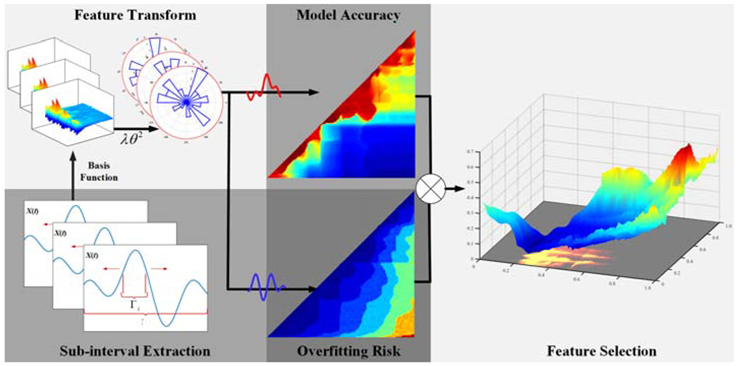
An illustration of our approach. Sub-Interval Extraction: sub-intervals are defined as candidate ROIs. Feature Transform: the functional feature of each candidate ROI is transformed using basis functions, e.g., eigenfunctions via FPCA. Two measures are proposed to evaluate the model accuracy and overfitting risk. Feature Selection: the ROI is selected as the subinterval that achieves the best trade-off between the two measures.

Model accuracy.

For each sub-interval Γ_j, we solve Eq.(4) by the least square method and obtain the coefficient estimates ${\widehat{\theta }}_i^{\mathrm{j}}$ and residual τ_j in Eq.(5), where Y is the vector of all subjects’ response vector, ${\widehat{\mathbf{Y}}}_j$ is the fitted response and ${\widehat{\mathit{\xi }}}_i^{\mathrm{j}}$ is the vector that consists of the i^th PC of all subjects.

$${\mathbf{\tau }}_{\mathit{j}}=\mathbf{Y}-{\widehat{\mathbf{Y}}}_j,{\widehat{\mathbf{Y}}}_j={\widehat{\alpha }}_0+\sum _{i=1}^{C_n^j}{\widehat{\theta }}_i^j{\widehat{\mathit{\xi }}}_i^j.$$ (5)

The model accuracy is measured by ${\widehat{v}}_j^2=\frac{{\tau }_j^T\tau }{n-1-C_n^j},$, the estimated noise variance in terms of the residual τ_j, which is commonly used in classical linear regression.

Overfitting risk.

A learning model trained with limited data is prone to suffer from overfitting, which means that it cannot be generalized well to unseen data. The larger the training dataset we use, the lower the overfitting risk. In theory, as the training data size increases, the training error converges to the generalization error and the overfitting risk converges to zero. We propose a novel measure to quantify the overfitting risk by evaluating the necessary sample size for the training model to achieve a sufficiently large statistical power. A small necessary sample size indicates a low risk of overfitting, whereas a large necessary sample size indicates a high risk. We will illustrate this relation using a real dataset in Section 4.3.

We follow [26] to obtain the sample size based on statistical power. First, we define

$${\widehat{V}}_i^j={\widehat{\lambda }}_i^j{\left({\widehat{\theta }}_i^j\right)}^2,i=1,2,\dots ,C_n^j.$$ (6)

The ${\widehat{V}}_i^{\mathrm{j}}$ is not only closely related to the coefficients of determination (i.e., R²) of the training model, but also takes the variation of PCs, i.e., ${\widehat{\lambda }}_i^{\mathrm{j}}$, into account. We denote their order statistics by ${\widehat{V}}_{\left(i\right)}^j$ in a decreasing order, with the concomitant coefficient estimate ${\widehat{\theta }}_{\left(i\right)}^j$ and PCs ${\widehat{\mathit{\xi }}}_{\left(i\right)}^j$.

Then we define a test statistic for the null hypothesis H₀ : β_j(t) = 0 for all t ∈ [0, 1] in Eq.(7) where γ is a pre-specified fraction, e.g., 0.95.

$$\{\begin{array}{c}{T}_j=\sum _{i=1}^{K_n^j}\frac{{\left({\widehat{\theta }}_{\left(i\right)}^j\right)}^2}{v\widehat{a}r\left({\widehat{\theta }}_{\left(i\right)}^j\right)}=\frac{1}{{\widehat{v}}_j^2}\sum _{i=1}^{K_n^j}\frac{{\left(Y^T{\widehat{\xi }}_{\left(i\right)}^j\right)}^2}{{\widehat{\xi }}_{\left(i\right)}^{jT}{\widehat{\xi }}_{\left(i\right)}^j};\\ K_n^j=\underset{S⩽C_n^j}{\arg \min }\left(\sum _{i=1}^S{\widehat{V}}_{\left(i\right)}^j/\sum _{i=1}^{C_n^j}{\widehat{V}}_{\left(i\right)}^j⩾\gamma \right).\end{array}$$ (7)

By Theorem 1 of [26], under the null hypothesis, the test function T_j in Eq.(7) is asymptotically equivalent to the sum of the first $K_n^j$ order statistics of $C_n^j$ independent chi-square random variables with degree of freedom 1. With the significance level α, let $q_{\left(\alpha ,K_n^j,C_n^j\right)}$ denote the 100(1 − α)% quantile of T_j under the null hypothesis, which can be found accurately by 10,000 Monte Carlo simulations.

By Theorem 2 of [26], under the significance level a, the necessary sample size h_j to achieve the statistical power p is determined by Eq.(8), where Φ is the cumulative distribution function of the standard normal distribution.

$$\{\begin{array}{c}1-\Phi \left(\frac{q_{\left(\alpha ,K_n^j,C_n^j\right)}-\left(K_n^j+\frac{h_j}{{\widehat{v}}_j^2}Z\right)}{\sqrt{2\left(K_n^j+2\frac{h_j}{{\widehat{v}}_j^2}Z\right)}}\right)⩾p;\\ Z=\sum _{i=1}^{K_n^j}{\widehat{V}}_{\left(i\right)}^j.\end{array}$$ (8)

Once h_j is obtained, the overfitting risk is measured by

$${\psi }_j=\log \left(\frac{h_j}{n}+1\right).$$ (9)

The risk ψ_j is always positive as in Eq.(9).

ROI selection.

We define a metric f which linearly trades off the normalized model accuracy and overfitting risk with the weight w as in Eq.(10).

$$\{\begin{array}{c}f\left({\psi }_j,{\widehat{v}}_j^2\right)=\left(1-w\right)P\left({\psi }_j\right)+wP\left({\widehat{v}}_j^2\right);\\ P\left(x\right)=\frac{x-\min \left(x\right)}{\max \left(x\right)-\min \left(x\right)}.\end{array}$$ (10)

For each sub-interval Γ_j, we compute a value of a $f\left({\psi }_j,{\widehat{v}}_j^2\right)$ following Eq.(10) and select the ROI of which f value is the smallest.

4. Discussion

The ROI is determined jointly by both model accuracy and overfitting risk via a weight w by Eq.(10). In this section we discuss how this weight influences the ROI selection in detail using a real dataset.

Dataset.

Some studies indicated the human body shape descriptors, such as the circumference and waist-hip ratio, can predict the visceral adipose tissue (VAT) value. We have collected a 3D human body shape data using a depth vision sensor (DVS) based 3D human body scan and reconstruct system [27]. The VAT value is measured by the CoreScan® (GE Healthcare, Madison, WI), a Dual-energy X-ray Absorptiometry (DXA) based VAT assessment software. The accuracy has been validated by multiple studies [28, 29]. Given the high cost of data collection, this is a very representative moderate-sized medical dataset, which contains 60 male and 87 female subjects. The body level circumference, one type of the anthropometric data, has been verified as a very useful shape descriptor to summarize body shape related information [30]. Therefore, we extract N = 128 equal-spaced level circumferences of the 3D body shape from the neck to the ankle (Figure 2–a). These level circumferences can be viewed as discrete measurements of a functional feature defined on the domain Γ = [0, 1]. The original functional feature derived from the level circumference is shown in Figure 2–b. We use the 60 male subjects to analyze the influence of the weight on the ROI selection.

Figure 2:

Functional features of the dataset. (a) Level circumference extraction from 3D body shape. (b) The original functional feature derived from the level circumference and the functional mean (the bold line) for male and female datasets respectively.

Implementation.

To study the effect of the weight w, we generate a real sequence ranging from 0.1 to 0.9 with the increment 0.1. A large w value implies an emphasis on model accuracy, while a small w implies an emphasis on suppressing overfitting. As the level circumference is measured at N = 128 points, for each value of the weight w, we traverse all 8128 ($C_{128}^2$) sub-intervals to locate the ROI following the procedures in Section 3.

We set the power p = 0.8, significance level α = 0.05, threshold η = 0.99 and threshold γ = 0.95, all of which are commonly used statistical parameter settings in hypothesis testing and functional data analysis [26].

4.1. Mix Weight

The heatmaps of the model accuracy and overfitting risk are illustrated in Figure 3. Unsurprisingly, their trends are reversed: a larger sub-interval corresponds to a more complex model and consequently, the model training error decreases while the overfitting risk increases. The heatmaps of the f function in Eq.(10) with different weights are shown in Figure 4. We also highlight the top candidate ROIs with the lowest 500 f values and their ranks have been color-coded.

Figure 3:

Heatmaps of the model accuracy(a) and the overfitting risk(b).

Figure 4:

ROI selection with different weights. (Top row) The f function heatmaps with different weights. (Bottom row) The distribution of the top 500 candidate ROIs corresponding to each heatmap.

As shown in Figure 4, a large weight attaches more importance to model accuracy and thus a wider ROI will be selected; however, a larger sub-interval results in a higher risk of overfitting. This is the reason why a weighted combination is desirable to achieve a balance. Nonetheless, there is no explicit reference on how to choose the best weight, since it is highly dependent on the data and training model. For our dataset, in Figure 5, we demonstrate the generalization error distribution of the models trained with functional features corresponding to different ROIs selected by different weight w. The generalization error is derived from the leave-one-out cross-validation (LOOCV). The difference between the best and the worst median absolute errors is over 30%. We find 0.5 is a reasonable weight. In general, if the sample size is large enough and the risk of overfitting is low, a larger weight works better and vice versa. Unless such knowledge is available, we recommend the weight 0.5 to practitioners.

Figure 5:

Boxplots for absolute errors of models with different weights. The red horizontal bar in each boxplot refers to the median.

4.2. Computational Cost Analysis

Our approach does not use the cross-validation process for ROI selection. Here we want to compare the computing time of our method with a cross-validation based method. In order to keep the results consistent, we choose the original cross-validation embedded in our functional linear regression model in Eq.(1). Meantime, we choose the mix weight w = 0.5 for our method. The K=5,6,7,8,9,10 folds cross-validation and LOOCV are compared in this section.

The results are shown in Table 1, which include the selected ROI, Root Mean Squared Error (RMSE), R-Squared value and execution time of each method in comparison. Table 1 shows that the execution time of the k-fold cross-validation is comparable with that of our method, but the ROI selected by the K-fold cross-validation is unstable for this small dataset as the partition to multiple folds is random. Thus one usually adopts LOOCV instead of K-folds cross validation for a small dataset. However, the LOOCV is unsurprisingly computationally very intensive, which as shown in Table 1 consumes the most execution time among all methods, more than six times than our proposed method. Without using cross-validation, our method is not sensitive to random partition as is the case for the K-fold cross-validation and does not suffer from intensive computation as is the case for the LOOCV.

Table 1:

The computation complexity analysis .

Case	ROI (t)	RMSE (in3)	R2	Exec.Time
5-folds	[0.102, 0.920]	1.530	0.720	129
6-folds	[0.086, 0.920]	1.523	0.721	144
7-folds	[0.141, 0.531]	1.449	0.749	161
8-folds	[0.156, 0.516]	1.420	0.758	184
9-folds	[0.165, 0.820]	1.559	0.709	203
10-folds	[0.117, 0.508]	1.549	0.713	216
LOOCV	[0.078, 0.508]	1.503	0.722	1168
Proposed	[0.148, 0.281]	1.348	0.782	178

4.3. Overfitting Risk, ROI and h_j

To verify the relation between the overfitting risk and necessary sample size to achieve a particular statistical power as in Section 3.2, we use the male VAT data for illustration. We randomly partition the data into a training set (80%) and a test set (20%). We consider two ROIs, [0.148, 0.281], the optimal ROI selected by our method, and the entire domain [0, 1]. Intuitively the second ROI [0, 1] is expected to overfit the data since it includes an additional but redundant domain compared to the first ROI. For each ROI, we fit a functional linear regression, calculate the training mean squared error (MSE) and test MSE, together with the overfitting risk (OR) OR = test MSE–training MSE. We also obtain the corresponding h_j following Eq.(8) using the training set, the necessary sample size to achieve power 0.8 with the level of significance 0.05. The results are given in Table 2.

Table 2:

The illustration of the relation between the overfitting risk and necessary sample size to achieve a particular statistical power using the male VAT data.

ROI	hj	Training MSE	Test MSE	OR
[0.148, 0.281]	92	0.458	1.715	1.257
[0, 1]	233	0.412	2.381	1.969

Table 2 shows that as expected the ROI [0, 1] leads to a larger overfitting risk since its corresponding OR value is larger, with a correspondingly larger h_j. This confirms the relation between the overfitting risk and necessary sample size to achieve a statistical power, that is, a small necessary sample size indicates a low risk of overfitting, whereas a large necessary sample size indicates a high risk.

5. Experiment

We compare our approach with other state-of-the-art FS methods. We choose six reference methods: Distance Correlation Selection (DCS) [16], RReliefF [17], Supervised Laplacian Score (SLS) [18], B-spline LASSO [14], Elastic-Net [31] and Step-wise feature selection [19]. The DCS, RReliefF and SLS are filter methods, the Step-wise feature selection is a wrapper method. The B-spline LASSO and Elastic-Net are both embedded methods. Among these six methods, only the B-spline Lasso is originally designed for functional ROI selection. The other methods are adapted to functional ROI selection, as discussed in Section 2. For each method, we will obtain the selected ROI and assess its prediction performance.

In addition to the female VAT data in our medical dataset in section 3, we also compare the performance of these methods when applied to the following three classical functional datasets.

Canadian Weather.

The dataset includes daily temperature and precipitation at 35 different locations in Canada averaged over 1960 to 1994 [8]. The daily temperature (annually 365 days) is continuously recorded and can be taken as the functional feature. The corresponding annual rainfall is the response. The temperatures in different days play different roles in regard to the annual rainfall. Therefore, we want to obtain the most predictive duration in a year (ROI of time) for the annual rainfall.

Moisture.

This data set consists of near-infrared reflectance spectra of 100 wheat samples, measured in 2 nm intervals from 1100nm to 2500nm and associated response variables, the samples’ moisture content [32]. The spectrum is very wide and varies continuously, which is considered as functional feature as well. We aim to find the most predictive spectrum band for the moisture.

DTI.

The diffusion tensor imaging data [33] consists of 100 subjects of Fractional anisotropy (FA) tract profiles for the corpus callosum (cca) and a score of the Paced Auditory Serial Addition Test (pasat). The dataset consists of 93 contiguous locations and we want to find the best area to associate the pasat score.

5.1. ROI Selection

For simplicity, the domain of the functional feature of each dataset above is transformed to [0, 1]. Without loss of generality, for our approach, we adopt the same statistical parameter settings as in Section 4 and let the mix weight w = 0.3, 0.5, 0.7 for comparison. We apply our method to the four datasets above and obtain the heatmaps of model accuracy, overfitting risk and f function, as shown in Figure 6. The ROI selected by our method with different weighted values (w = 0.3, 0.5, 0.7) for these four datasets and corresponding p-values are also included in Figure 6. Thus all functional features defined on their corresponding ROIs in the four datasets have significant predictabilities at the significance level 0.05.

Figure 6:

The results of our approach applied to the VAT dataset, Canadian Weather (CW) dataset and Moisture (MO) dataset. (a) The overfitting risk heatmap. (b) The model accuracy heatmap. (c) (e) The f function heatmap and the selected ROI (the magenta cross) with w = 0.3, 0.5, 0.7. (f) The top 500 ranked candidate ROIs with w = 0.5.

Meanwhile, we also apply the six reference methods to these datasets. Figure 7 illustrates the ROIs selected by the six reference methods according to the coefficient function β(t). We draw the weights of the β(t) and color encodes the significance of the whole domain. Obviously these selected ROIs in each dataset are very different. For the VAT dataset experiment, only our method and SLS are able to pick up the sub-interval [0.406, 0.469], which is abdomen to hip, a critical region for the VAT prediction [34]. For the Canadian Weather dataset, according to Ramsay and Silverman [8], the temperature between October to November([0.8, 0.9]) is the most significant factor in influencing the annual precipitation. Our method selects the period between late summer and fall. The spectrum analysis often focuses on a narrow band and our method is able to extract the ROI ([0.023, 0.086]) in the Moisture data, which is a relatively narrow region. For the DTI dataset, it seems the region ([0.2, 0.4]) is more effective[35], and the reference methods usually include region ([0.5, 1]). It is worth mentioning that for these four datasets, the reference methods cannot guarantee localization of the estimated coefficient function β(t) to zero-out irrelevant regions effectively, whereas our method overcomes this limitation.

Figure 7:

ROIs selected by the reference methods: (a) DCS, (b) RReliefF, (c) SLS, (d) B-spline LASSO, (e) Elastic-Net and (f) Step-wise, according to the coefficient function β(t). The blue region corresponds to high coefficient values; the red region corresponds to the low coefficient values; the gray curve corresponds to the coefficient function.

5.2. Prediction

For each dataset, it is very difficult to identify the ground truth ROI without any prior knowledge. Therefore, we evaluate the performance of the selected ROIs in terms of predicting the response using the functional linear model in Eq.(1). For example, for the ROI selected by each method, we set I = I_select in Eq.(1). We then calculate the R-Squared and Root Mean Squared Error (RMSE) of prediction based on LOOCV. The extracted ROIs of all datasets above by different approaches and evaluated reults are shown in Table 3. The prediction absolute errors are illustrated in Figure 8. We can conclude that our proposed method is almost always superior compared with the reference methods. The performance of our method with different weight values w = 0.3, 0.5, 0.7, is slightly different. In comparison, w = 0.7 works the worst in all datasets, w = 0.5 performs best in Moisture dataset and w = 0.3 is the best in the other three datasets. For the Canadian Weather data, in terms of RMSE and R Squared, our proposed method is only slightly worse than DCS and RReliefF, but better than the others. With respect to the Medical, Moisture and DTI datasets, our method is better than all other methods, with both the smallest RMSE and largest R-Squared values. The four experiments show that our approach can effectively locate the ROI of a the functional feature in the context of functional linear regression.

Table 3:

The comparison of prediction performance. Note: The Canadian Weather Datasets is cyclic recorded, thus it allow the boundary larger than 1.

Dataset	Methods	ROI	RMSE	R-Squared
	DCS	[0.172, 0.336]	1.356	0.667
	RReliefF	[0.156, 0.383]	1.367	0.662
	SLS	[0.406, 0.578]	1.419	0.635
Medical	LASSO	[0.180, 0.328]	1.356	0.665
	Elastic-Net	[0.188, 0.328]	1.359	0.656
	Step-wise	[0.141, 0.352]	1.384	0.653
	Proposed(w = 0.3)	[0.223, 0.305]	1.006	0.770
	Proposed(w = 0.5)	[0.289, 0.469]	1.105	0.746
	Proposed(w = 0.7)	[0.117, 0.516]	1.326	0.677
	DCS	[0.835, 1.016]	4.314	0.729
	RReliefF	[0.853, 1.022]	4.402	0.718
Canadian	SLS	[0.359, 0.444]	5.272	0.596
Weather	LASSO	[0.674, 0.805]	5.081	0.625
	Elastic-Net	[0.833, 1.041]	4.633	0.688
	Step-wise	[0.882, 0.978]	4.709	0.678
	Proposed(w = 0.3)	[0.533, 0.854]	4.474	0.710
	Proposed(w = 0.5)	[0.574, 0.859]	4.415	0.709
	Proposed(w = 0.7)	[0.423, 0.849]	4.736	0.679
	DCS	[0.000, 0.024]	0.921	0.554
	RReliefF	[0.417, 0.549]	0.821	0.646
	SLS	[0.291, 1.000]	0.823	0.645
Moisture	LASSO	[0.528, 0.629]	0.852	0.619
	Elastic-Net	[0.531, 0.618]	0.853	0.618
	Step-wise	[0.514, 0.606]	0.845	0.625
	Proposed(w = 0.3)	[0.071, 0.109]	0.789	0.673
	Proposed(w = 0.5)	[0.023, 0.086]	0.733	0.717
	Proposed(w = 0.7)	[0.032, 0.124]	0.877	0.610
	DCS	[0.398, 0.505]	6.014	0.732
	RReliefF	[0.957, 1.000]	7.004	0.637
	SLS	[0.860, 0.925]	6.561	0.681
DTI	LASSO	[0.333, 0.516]	6.412	0.695
	Elastic-Net	[0.323, 0.538]	6.428	0.694
	Step-wise	[0.376, 0.505]	6.328	0.7.0
	Proposed(w = 0.3)	[0.140, 0.452]	5.647	0.764
	Proposed(w = 0.5)	[0.033, 0.482]	5.906	0.742
	Proposed(w= 0.7)	[0.108, 0.796]	6.804	0.657

Figure 8:

The absolute errors based on LOOCV of all methods in comparison. The a - i are DCS, RReliefF, SLS, LASSO, Elastic-Net, Step-wise and Proposed method(w = 0.3,w = 0.5,w = 0.7) .

6. Conclusion

This paper proposes an effective ROI selection method for functional features. Our proposed method provides a novel metric to balance model accuracy and overfitting risk. Under the framework of functional linear regression, the model accuracy is measured by the residual variance, while the overfitting risk is quantified through the necessary sample size to achieve a certain statistical power. We have evaluated the performance of our proposed method on four representative moderate sized datasets and compared it with six state-of-the-art reference methods. The proposed method almost always outperforms other reference methods.

The proposed framework may be generalized to other scenarios. First, it may be extended to ROI selection for multi-dimensional functional features, although in this paper we only illustrate its application to one-dimensional functional data. Similar to Theorem 2 of [26], the relationship between the sample size and statistical power for multi-dimensional functional linear regression may be attainable, which makes our method generalizable. One caveat is that it is impractical to exhaust all possible sub-intervals to select the optimal ROI for multi-dimensional functional features. Thus a more efficient search algorithm is needed, which is an interesting future research direction. Moreover, our proposed method can be adapted to nonlinear functional regression models as long as corresponding valid sample size estimation methods can be developed. Such extension requires substantial theoretical analyses, which are beyond the scope of this paper.

Our framework assumes independently and identically distributed (i.i.d.) data. This assumption is valid most of the time if the data are collected from a random sample from a population, so our proposed method is generally applicable to such data. When feature selection tasks arise from non i.i.d. data, such as time series, our proposed method may not be applicable or perform poorly.

References

- [1].Jian L, Li J, Shu K, Liu H, Multi-label informed feature selection., in: IJCAI, 2016, pp. 1627–1633. [Google Scholar]
- [2].Hara S, Maehara T, Enumerate lasso solutions for feature selection, in: AAAI, 2017, pp. 1985–1991. [Google Scholar]
- [3].Roffo G, Melzi S, Castellani U, Vinciarelli A, Infinite latent feature selection: A probabilistic latent graph-based ranking approach, in: Computer Vision and Pattern Recognition, 2017. [Google Scholar]
- [4].Chang X, Nie F, Yang Y, Huang H, A convex formulation for semi-supervised multi-label feature selection., in: AAAI, 2014, pp. 1171–1177. [Google Scholar]
- [5].Bertsimas D, King A, Mazumder R, et al. , Best subset selection via a modern optimization lens, The annals of statistics 44 (2) (2016) 813–852. [Google Scholar]
- [6].Kohavi R, A study of cross-validation and bootstrap for accuracy estimation and model selection, in: Ijcai, Vol. 14, Montreal, Canada, 1995, pp. 1137–1145. [Google Scholar]
- [7].Rao RB, Fung G, Rosales R, On the dangers of cross-validation. an experimental evaluation, in: Proceedings of the 2008 SIAM International Conference on Data Mining, SIAM, 2008, pp. 588–596. [Google Scholar]
- [8].Ramsay J, Silverman B, Functional data analysis, Springer Series in Statistics, 2005. [Google Scholar]
- [9].Ferraty F, Vieu P, Nonparametric functional data analysis: theory and practice, Springer Science & Business Media, 2006. [Google Scholar]
- [10].Horváth L, Kokoszka P, Inference for functional data with applications, Vol. 200, Springer Science & Business Media, 2012. [Google Scholar]
- [11].Hsing T, Eubank R, Theoretical foundations of functional data analysis, with an introduction to linear operators, John Wiley & Sons, 2015. [Google Scholar]
- [12].Wang J-L, Chiou J-M, Müller H-G, Functional data analysis, Annual Review of Statistics and Its Application 3 (2016) 257–295. [Google Scholar]
- [13].Zhang X, Wang J-L, From sparse to dense functional data and beyond, The Annals of Statistics 44 (5) (2016) 2281–2321. [Google Scholar]
- [14].James GM, Wang J, Zhu J, et al. , Functional linear regression that’s interpretable, The Annals of Statistics 37 (5A) (2009) 2083–2108. [Google Scholar]
- [15].Zhou J, Wang N-Y, Wang N, Functional linear model with zero-value coefficient function at sub-regions, Statistica Sinica 23 (1) (2013) 25. [DOI] [PMC free article] [PubMed] [Google Scholar]
- [16].Li R, Zhong W, Zhu L, Feature screening via distance correlation learning, Journal of the American Statistical Association 107 (499) (2012) 1129–1139. [DOI] [PMC free article] [PubMed] [Google Scholar]
- [17].Robnik-Šikonja M, Kononenko I, Theoretical and empirical analysis of relieff and rrelieff, Machine learning 53 (1-2) (2003) 23–69. [Google Scholar]
- [18].Chen X, Yuan G, Nie F, Huang JZ, Semi-supervised feature selection via rescaled linear regression., in: IJCAI, Vol. 2017, 2017, pp. 1525–1531. [Google Scholar]
- [19].Draper NR, Smith H, Applied regression analysis, Vol. 326, John Wiley & Sons, 2014. [Google Scholar]
- [20].Tibshirani R, Regression shrinkage and selection via the lasso, Journal of the Royal Statistical Society. Series B (Methodological) (1996) 267–288. [Google Scholar]
- [21].Zou H, Hastie T, Regularization and variable selection via the elastic net, Journal of the Royal Statistical Society: Series B (Statistical Methodology) 67 (2) (2005) 301–320. [Google Scholar]
- [22].Xu Z, Huang G, Weinberger KQ, Zheng AX, Gradient boosted feature selection, in: Proceedings of the 20th ACM SIGKDD international conference on Knowledge discovery and data mining, ACM, 2014, pp. 522–531. [Google Scholar]
- [23].Chen S-B, Zhang Y, Ding CH, Zhou Z-L, Luo B, A discriminative multi-class feature selection method via weighted l2, 1-norm and extended elastic net, Neurocomputing 275 (2018) 1140–1149. [Google Scholar]
- [24].Litany O, Remez T, Rodola E, Bronstein A, Bronstein M, Deep functional maps: Structured prediction for dense shape correspondence, in: 2017 IEEE International Conference on Computer Vision (ICCV), IEEE, 2017, pp. 5660–5668. [Google Scholar]
- [25].Ghiasi G, Fowlkes CC, Laplacian pyramid reconstruction and refinement for semantic segmentation, in: European Conference on Computer Vision, Springer, 2016, pp. 519–534. [Google Scholar]
- [26].Su Y-R, Di C-Z, Hsu L, Hypothesis testing in functional linear models, Biometrics 73 (2) (2017) 551–561. [DOI] [PMC free article] [PubMed] [Google Scholar]
- [27].Lu Y, Zhao S, Younes N, Hahn JK, Accurate nonrigid 3d human body surface reconstruction using commodity depth sensors, Computer Animation and Virtual Worlds 29 (5) (2018) e1807. [DOI] [PMC free article] [PubMed] [Google Scholar]
- [28].Mohammad A, Rolfe EDL, Sleigh A, Kivisild T, Behbehani K, Wareham NJ, Brage S, Mohammad T, Validity of visceral adiposity estimates from dxa against mri in kuwaiti men and women, Nutrition & diabetes 7(1) (2017) e238. [DOI] [PMC free article] [PubMed] [Google Scholar]
- [29].Neeland I, Grundy S, Li X, Adams-Huet B, Vega G, Comparison of visceral fat mass measurement by dual-x-ray absorptiometry and magnetic resonance imaging in a multiethnic cohort: the dallas heart study, Nutrition & diabetes 6 (7) (2016) e221. [DOI] [PMC free article] [PubMed] [Google Scholar]
- [30].Lu Y, McQuade S, Hahn JK, 3d shape-based body composition prediction model using machine learning, in: 2018 40th Annual International Conference of the IEEE Engineering in Medicine and Biology Society (EMBC), IEEE, 2018, pp. 3999–4002. [DOI] [PMC free article] [PubMed] [Google Scholar]
- [31].Wang J, Shen J, Li P, Provable variable selection for streaming features, in: International Conference on Machine Learning, 2018, pp. 5158–5166. [Google Scholar]
- [32].Reiss PT, Ogden RT, Functional principal component regression and functional partial least squares, Journal of the American Statistical Association 102 (479) (2007) 984–996. [Google Scholar]
- [33].Goldsmith J, Crainiceanu CM, Caffo B, Reich D, Longitudinal penalized functional regression for cognitive outcomes on neuronal tract measurements, Journal of the Royal Statistical Society: Series C (Applied Statistics) 61 (3) (2012) 453–469. [DOI] [PMC free article] [PubMed] [Google Scholar]
- [34].Snijder M, Van Dam R, Visser M, Seidell J, What aspects of body fat are particularly hazardous and how do we measure them?, International journal of epidemiology 35 (1) (2005) 83–92. [DOI] [PubMed] [Google Scholar]
- [35].Goldsmith J, Bobb J, Crainiceanu CM, Caffo B, Reich D, Penalized functional regression, Journal of Computational and Graphical Statistics 20 (4) (2011) 830–851. [DOI] [PMC free article] [PubMed] [Google Scholar]