An evaluation of the performance of selected (Q)SARs/expert systems for predicting acute oral toxicity

Abstract

Multiple US agencies use acute oral toxicity data in a variety of regulatory contexts. One of the ad-hoc groups that the US Interagency Coordinating Committee on the Validation of Alternative Methods (ICCVAM) established to implement the ICCVAM Strategic Roadmap was the Acute Toxicity Workgroup (ATWG) to support the development, acceptance, and actualisation of new approach methodologies (NAMs). One of the ATWG charges was to evaluate in vitro and in silico methods for predicting rat acute systemic toxicity. Collaboratively, the NTP Interagency Center for the Evaluation of Alternative Toxicological Methods (NICEATM) and the US Environmental Protection Agency (US EPA) collected a large body of rat oral acute toxicity data (~16,713 studies for 11,992 substances) to serve as a reference set to evaluate the performance and coverage of new and existing models as well as build understanding of the inherent variability of the animal data. Here, we focus on evaluating in silico models for predicting the Lethal Dose (LD50) as implemented within two expert systems, TIMES and TEST. The performance and coverage were evaluated against the reference dataset. The performance of both models were similar, but TEST was able to make predictions for more chemicals than TIMES. The subset of the data with multiple (>3) LD50 values was used to evaluate the variability in data and served as a benchmark to compare model performance. Enrichment analysis was conducted using ToxPrint chemical fingerprints to identify the types of chemicals where predictions lay outside the upper 95% confidence interval. Overall, TEST and TIMES models performed similarly but had different chemical features associated with low accuracy predictions, reaffirming that these models are complementary and both worth evaluation when seeking to predict rat LD50 values.

1. Introduction

Acute oral toxicity testing is conducted to determine the immediate health effects of an orally administered chemical substance and is expressed in terms of the lethal dose that kills 50% (LD50) of the animals tested [1]. Acute oral toxicity data are used by US agencies in a variety of regulatory contexts including hazard classification and labelling of pesticide products, determining acceptable human exposure limits and personal protective equipment needed for handling, or determining counter measures that should be employed in the event of toxic exposures [1–3]. Acute oral toxicity data may also be used to establish doses administered during repeat dose toxicity studies, identify target organs for toxicity, and assess the hazard of accidental ingestions of chemical contaminants in food [1]. To date, there are no in vitro tests accepted by regulatory agencies as stand-alone replacements for acute oral animal tests [1,4]. Several US government agencies participate in the Interagency Coordinating Committee on the Validation of Alternative Methods (ICCVAM), which established an ad-hoc workgroup, the Acute Toxicity Work Group (ATWG), to develop an implementation plan for identifying, evaluating, and applying new approach methodologies that may serve as replacements for in vivo acute systemic toxicity studies. Two key elements of this implementation plan are: 1) acquiring and curating a high-quality reference dataset of acute oral toxicity data; and 2) identifying, developing, and evaluating non-animal alternative approaches. Here, we sought to evaluate selected existing legacy expert systems for the prediction of acute oral systemic toxicity (i.e. LD50), to complement a global project that had been initiated to develop new in silico models [5]. A number of models have been developed in the past that facilitate predictions of acute oral toxicity, notable software tools where these models have been implemented include the TopKat model first developed by Enslein et al [6], HazardExpert [7], ACD/Percepta [8], CASE Ultra [9] and the OECD Toolbox [10]. Further, there are many models that have been developed using a plethora of different machine learning approaches – from linear regressions [11] to random forests [12], support vector machines [12] and k-nearest neighbours [13]. Deep learning approaches have also been used [14]. In this study, two existing models were accessible: the Toxicity Estimated Software (TEST), a statistical expert system which uses a variety of Quantitative Structure Activity Relationship (QSAR) models [15], and the commercial hybrid expert system, Tissue Metabolism Simulator (TIMES), which comprises a collection of chemical/mechanistic category based Structure-Activity Relationships (SARs) underpinned by QSARs [16]. The performance of both models was assessed using the reference dataset that had been assembled under the auspices of the ATWG.

The TIMES expert system contains an acute oral toxicity model that was based on a training set of rodent (predominantly rat) LD50 values for 1814 chemicals. The TIMES approach relies on a baseline model for substances that are neutral organics. Substances possessing features that can exert toxicity beyond that predicted by the baseline toxicity QSAR are assigned into one of 73 toxicological categories underpinned by a specific QSAR. These QSARs are, in some cases, associated with an established molecular initiating event within an Adverse Outcome Pathway (AOP)-like construct (since published in [16]). TIMES has a self-reported coefficient of determination (R²) of 0.85 with a Mean Squared Error (MSE) of 0.15 for the training set of 1814 chemicals (as noted in the summary model description within the TIMES software itself, no further information was provided as far as whether this was a cross validation result).

The TEST expert system relies on a range of different QSAR methods, some local based (e.g. nearest neighbour) and some global based from which a consensus prediction is derived and reported as an overall outcome. For acute oral toxicity, 3 methods are used, hierarchical clustering, FDA, method and nearest neighbour from which the consensus prediction is derived. To create the training set for TEST, oral rat LD50 values were obtained by downloading records from the ChemIDplus database [15]. A total of 13,548 records were obtained using the following search criteria – test: LD50, species: rat, route: oral. Substances were subsequently filtered to remove inorganics, organometallics, and mixtures such that the final oral rat LD50 set comprised 7413 chemicals and the endpoint modelled was the −log10 (LD50 mol/kg). TEST model developers determined it was not possible to develop a single model or group contribution model to fit the entire training set, therefore, three models were developed. The first TEST model used hierarchical clustering and the second used the FDA method and the third, a nearest neighbours approach, a consensus was then used to derive an overall prediction. The reported performance characteristics for the TEST consensus model for the external test set were R²: 0.626, Root Mean Standard Error (RMSE): 0.594 and Mean Absolute Error (MAE): 0.431 (as reported in the User Manual: see https://www.epa.gov/chemical-research/users-guide-test-version-42-toxicity-estimation-software-tool-program-estimate; [15]). In this evaluation, only predictions with a consensus value were used in the assessment of performance.

The current study sought to compare the predictions from TEST and TIMES (that were not part of their respective training sets) through using the reference set compiled under the auspices of the ICCVAM ATWG. Using such a large experimental reference dataset enabled a broader evaluation of the prediction models, informing on domain of applicability restrictions in a way never previously explored.

2. Methods

2.1. Acute Toxicity dataset

The rat acute oral systemic toxicity dataset assembled by the ICCVAM ATWG served as the reference LD50 values against which the predictions from the two models were compared. This dataset is comprised of 21,200 LD50 values (15,688 unique substances), including both point estimate (14,745) and limit test (6,455) values. These data were collated from a variety of publicly available databases and resources, including from OECD’s eChemPortal, JRC’s Acutetoxbase, and ChemIDplus ([5]; https://ntp.niehs.nih.gov/go/tox-models).

Subsequently, the original dataset was processed to: 1) identify and remove duplicate study values, due to the same study being present in multiple sources; 2) amend obvious transcriptions errors, e.g. an LD50 limit test given as “20005000 mg/kg”; and 3) retrieve structure information primarily from the US EPA’s CompTox Chemicals Dashboard (https://comptox.epa.gov, [17–18]) and other public resources. More information regarding these processing steps can be found in https://ntp.niehs.nig.gov/iccvam/at-models-2018/ppt/4-karmaus.pdf. Together, this process reduced the number of LD50 values to 16,209 associated with 11,992 unique substances.

Finally, for chemicals with multiple point estimates (at least 3), a representative LD50 value (called the processed LD50 throughout the remainder of this manuscript) was identified by calculating the median of the lowest quartile. This involved removing “extreme” point estimate values outside the Tukey fence (i.e. exceeding 1.5 * interquartile range) and, subsequently, deriving the median of the recalculated lower 25^th percentile of the remaining values. Therefore, the final processed acute toxicity dataset (herein termed the processed reference dataset) consisted of 11,992 unique substances with an acute toxicity outcome, 8979 of these had a computed processed LD50.

2.2. Chemical structure data

The structures retrieved as part of the ICCVAM ATWG effort yielded information for 11,992 substances, by integrating information from multiple sources. Therefore, to ensure the chemical structures were consistent and of a high quality, only those substances with QSAR-ready simplified molecular-input line entry (SMILES) in the EPA’s Distributed Structure-Searchable Toxicity (DSSTox) database [17–18] were retained. Furthermore, using the QSAR-ready SMILES offered the additional advantage of having SMILES strings that were already desalted and neutralised; thereby, facilitating the profiling of the compounds through the two expert systems. To retrieve this information, a batch search of the EPA CompTox Chemicals Dashboard (www.comptox.epa.gov/dashboard) was performed utilising the Chemical Abstract Services (CAS) registration numbers (www.cas.org) as inputs. In addition to the QSAR-ready SMILES, DSSTox substance identifiers (DTXSID), chemical names, regular SMILES strings, and average mass information for each substance were also extracted. This reduced the number of chemicals that were carried forward for analysis to 10,886. Subsequently, the QSAR-ready SMILES were read into MarvinView (v18.28, ChemAxon Ltd.) and saved as a structure data (SD) file (.sdf).

Finally, the ChemoTyper software (https://chemotyper.org/) was used to create a 729-bit binary molecular fingerprint for each chemical in the processed dataset using the ToxPrint chemotype feature set (v2.0_r711) (see section 2.5) to facilitate the enrichment analysis.

2.3. Profiling substances through prediction software

2.3.1. Toxicity Estimation Software Tool (TEST)

To facilitate computational processing of the TEST (v4.2.1) predictions, the input SD file was split into multiple SD files using a “SDFBreaker” Python script. The split was arbitrarily set at 250 chemicals per SD file as a pragmatic size to use for processing. For each batch of chemicals, the oral rat LD50 was selected as the endpoint of interest and the TEST consensus method was chosen to run the predictions. The output file ‘all methods’ was downloaded which contained the predictions from the different QSAR methods, as well as the consensus prediction expressed in units of −log10(mol/kg). The consensus method estimates the LD50 value by calculating an average of the predicted toxicity from the aforementioned QSAR methods. More information about each of these approaches can be found in the TEST user guide (https://epa.gov/sites/production/files/2016-05/documents/600r16058.pdf). In instances where only one of the three QSAR methods can make a prediction, that prediction is deemed to be unreliable by TEST and, thus, a consensus prediction cannot be made. The results from each batch of 250 chemicals were saved in a separate text file to be concatenated later.

2.3.2. Tissue Metabolism Simulator (TIMES)

The “SDFBreaker” python script was also used to split the original SD file into batches containing 1000 chemicals to be used to make predictions in TIMES. NB: Past experience found that 1000 chemicals as a batch limit did not cause any memory issues during processing. For each SD file that was run through TIMES (v2.28.1.6), the SD file was first converted into ODB (OpenOffice database) format, selecting CAS, DTXSID, and chemical name as synonyms. Default settings for both the 2-D conversion mode for converting the chemical structure and for the physicochemical properties (logK_OW and water solubility) were used. Once the chemicals had been imported, the acute oral toxicity (v10) model was loaded and used to profile each chemical. The predictions derived from each batch were exported as separate tsv files to be concatenated later.

2.4. Assessing performance of software predictions

2.4.1. Calculation of residuals

To facilitate the performance assessment, only predictions for chemicals that were not part of the underlying training sets were considered from the 2 expert systems. This involved the following steps; first chemicals from the processed reference dataset (11,992 chemicals) were gathered and DSSTox structures were identified. Next, chemicals were dropped if either the TEST or TIMES dataset was unable to derive a LD50 prediction. For TEST, this was because no consensus model prediction could be derived. For TIMES, this was because a substance was not captured by any of the predefined toxicological categories. Chemicals that formed part of the training sets for each model were also dropped. Both datasets were then merged with the processed reference dataset, removing any chemicals for which a processed LD50 value was unavailable. The resulting dataset comprised a known (experimental) LD50 value (the processed LD50 value) and associated predictions from TEST or TIMES that did not form part of the training sets. Figure 1 represents the workflow for creation of the datasets.

Figure 1.

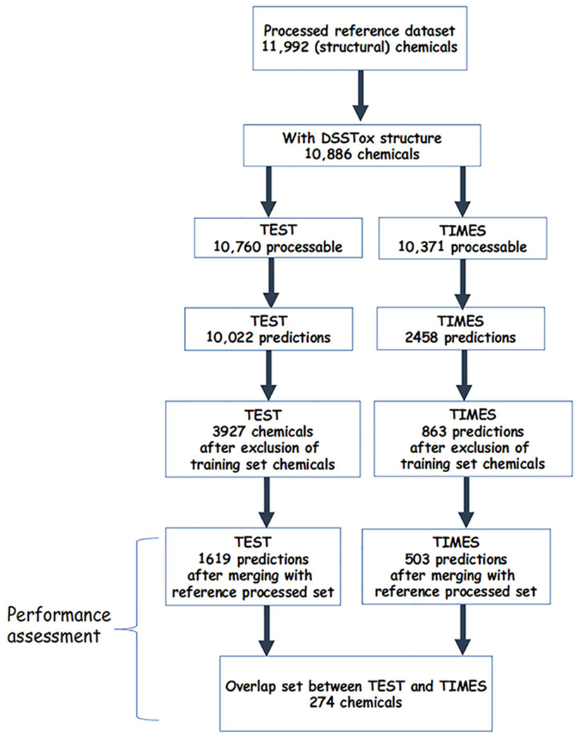
Workflow for creating the TEST and TIMES datasets.

The output for predictions generated by the TEST and TIMES models were not reported in the same units. TEST returned predictions in −log10(mol/kg) format using the ‘all methods batch export’, whereas TIMES predictions were reported in units of mg/kg. The compiled experimental rat oral acute systemic toxicity values were also reported in units of mg/kg. Consequently, all known and predicted LD50 values were converted into their -log molar equivalents (termed pLD50) using Equation 1.

$$\mathit{pLD}50=-{\mathit{log}}_{10}(\mathit{LD}50(\mathit{mg}∕\mathit{kg})∕\mathit{MW}(g∕\mathit{mol})∕1000)$$ (1)

where LD50 is the oral LD50 of the chemical (in mg/kg) and MW is the average mass of the chemical (in g/mol).

Residuals were then calculated for each chemical with a pLD50 prediction by subtracting the predicted pLD50 from the experimental processed pLD50, using Equation 2.

$${\text{Residual}}_i=\mathit{ExpLD}{50}_i-\mathit{PredLD}{50}_i$$ (2)

2.4.2. Calculating confidence intervals of experimental LD50 values

To benchmark the performance of the predicted LD50s compared with the experimental values, it was important to understand the inherent variability of the experimental animal data, i.e. how reproducible an LD50 value was for a given substance. Here, the original rat acute oral toxicity dataset (comprising 21,200 LD50 values for 15,688 substances) was filtered to create two subsets: 1) retaining all chemicals with three or more LD50 values (termed the complete subset), and 2) retaining only those chemicals with three or more LD50 values and average mass information (termed the ‘average mass subset’). For the average mass subset, Equation 1 was used to convert the experimental data from mass units (i.e. mg/kg) to -log molar units (i.e. −log10(mol/kg)).

To compare the variability of the average mass subset relative to the complete subset, an overall standard deviation was calculated (in log10(mg/kg)). The standard deviations across all chemicals in the subset were then bootstrapped using 10,000 replicates with replacement. The mean of the bootstrapped standard deviations were used to derive a 95% confidence interval (CI). Figure 2 outlines the workflow for the variability assessment.

Figure 2.

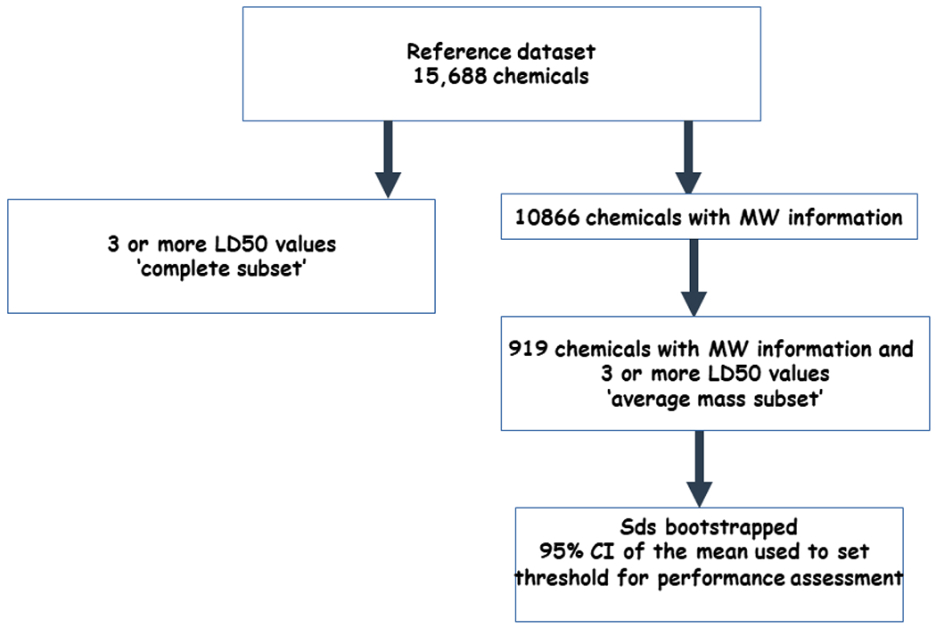
Workflow to create the dataset for the CI threshold.

2.4.3. Assessment of the model predictions

The performance of the predictions generated by the TEST and TIMES models were evaluated in a number of different ways. The first involved comparing the chemical-specific residuals to the upper 95% CI value of the mean of the bootstrapped standard deviations by the total number of chemicals and their percentage. Additionally, the goodness of fit measures between the predicted and experimental LD50s were calculated, namely: the median absolute error (MAE), the root mean squared error (RMSE), and the coefficient of determination (R²). The Pearson correlation coefficient for each set of pairwise complete observations were also computed to compare how correlated the predictions were to the experimental values and each other. These metrics were calculated both for the total number of chemicals with a prediction from the TEST or TIMES (not part of the respective training set), as well as the chemicals with a prediction from both TEST and TIMES (i.e. the overlapping chemicals).

2.5. Investigation of chemical space

Chemotype enrichment analysis was conducted to investigate if there were areas of chemical space where each model was best or poor at making predictions. Readers are directed to [19] for a more comprehensive explanation of the chemotype enrichment analysis workflow used in this study. Briefly, chemotype enrichment analysis identifies sub-structural features (i.e. amongst the 729 ToxPrint chemotypes) that are over-represented with respect to a given endpoint. Here, the “endpoint” in question is whether the model prediction for a chemical was beyond the 95% confidence interval of the variability of the experimental data as calculated in section 2.4.2.

The chemotype enrichment analysis was performed separately for the TEST and TIMES models. To conduct this analysis, the ChemoTyper software (https://chemotyper.org/) was used to generate a 729-bit binary molecular fingerprint for all chemicals with a QSAR-ready SMILES string based on the publicly available ToxPrint feature set (https://toxprint.org). Next, a new bit was appended to the ToxPrint fingerprints that accounted for whether or not the software prediction was within the variability of the experimental data using the upper 95% CI as a threshold, indicated by 1 or 0. For each model, chemicals whose predictions were outside of the 95% confidence interval of experimental variability were indicated by a value of 1, whilst chemicals whose predictions were within the 95% confidence interval of experimental variability were indicated by a value of 0. The odds ratio (OR) and associated p-value metrics were calculated to identify the ToxPrints that were more highly enriched for the predictions outside of the confidence interval of the experimental variability compared to the predictions within the experimental variability. For a ToxPrint to be considered enriched, it required 3 or more true positives (TP) (i.e. prediction outside confidence interval and presence of the ToxPrint), an OR of ≥2.5, and a p-value of ≤0.05. As a final step the probabilities of the presence of a ToxPrint outside of the confidence interval (TP/TP+FP, otherwise known as the precision) was computed for both models and a ratio taken in order to derive a confidence metric. This confidence metric was intended to provide a quantitative measure of the relative confidence of which of the 2 models was preferable for use based on the set of their respective ToxPrints. A handful of illustrative examples are provided to demonstrate this potential approach.

2.6. Data analysis software and code

Data processing was conducted using the Anaconda distribution of Python 3.8 (Anaconda.org) and associated libraries – scikit-learn, pandas, numpy, visualisation tools: matplotlib and seaborn and the statistical library scipy within a Jupyter lab environment. Python Jupyter Notebooks and datasets are available on the EPA FTP website (ftp://newftp.epa.gov/COMPTOX/CCTE_Publication_Data/)

3. Results and Discussion

3.1. Overall results

QSAR-ready SMILES and average mass, were available in the EPA CompTox Chemicals Dashboard for 10,886 of the 11,992 substances in the processed reference dataset. However, not all of the chemicals with QSAR-ready SMILES could be processed through the two models: TEST was able to process 10,760 chemicals, whereas TIMES was able to process 10,371 chemicals, due to constraints in the clustering/profiling approaches within both models. TEST was able to make a LD50 prediction for the vast majority of chemicals that it was able to process (93.1% or 10,022 chemicals); TIMES, meanwhile, was only able to make a prediction for less than a quarter of the chemicals it was able to process (23.8% or 2,458 chemicals) (Table 1). After removal of chemicals that were part of the TEST training set, the number of chemicals with a LD50 prediction was reduced to 3,927 (36.5% of the processed reference dataset chemicals). Removal of chemicals with LD50 predictions that made up the training set for the TIMES software resulted in 863 chemicals (8.3% of the processed chemicals) being retained. Combining the chemicals with predictions that did not make up the training set of the model with chemicals from the processed reference dataset with an experimental LD50 value resulted in a final dataset of 1,621 chemicals with a TEST prediction and 503 chemicals with a TIMES prediction. Therefore, purely based on counts, TEST was able to make predictions for more chemicals than TIMES. It is important to note that the low numbers are not indicative of the applicability of the models but rather the large overlap between the identity of the training set chemicals and that of the processed reference dataset.

Table 1.

Counts of chemicals with QSAR Ready SMILES run through TEST and TIMES

	TEST	TIMES
Total chemicals amenable to processing for prediction	10760	10371
Chemicals with LD50 prediction (not in training set)	3927	863

3.2. Investigation of variability of experimental data

In order to have a relative benchmark to compare the performance of the predictions obtained from the TEST and TIMES models, it was important to gain an understanding of the inherent variability existing in the experimental animal data using replicate study data per chemical. This involved taking the original rat oral acute systemic toxicity dataset of 21,200 LD50 values (15,688 unique substances) and merging it with average mass information (10,886 chemicals with 14,964 LD50 values). Next the dataset was filtered to retain only those substances with three or more LD50 values (this included both limit and point estimate values). After applying these filtering criteria, a total of 4,198 LD50 values, covering 919 unique substances, were retained. Approximately 90% of the substances were associated with between 3 and 5 LD50 values, with one chemical (peracetic acid) having 57 unique LD50 values.

The standard deviation of the LD50 values for the average mass subset of chemicals was also compared to the set of chemicals with three or more LD50 values where average mass information was not necessarily available. The standard deviation (in log10(mg/kg)) was 0.828 for the complete subset of chemicals with three or more LD50 values, whereas it was 0.842 for the average mass subset. Based on the apparent lack of difference, the assumption made was that the average mass subset was sufficiently representative of the ‘complete subset’. Accordingly, the standard deviation of the average mass subset was then bootstrapped using 10,000 replicates and the mean and 95% confidence interval (CI) of the resulting bootstrapped distribution was derived. The mean of the bootstrapped standard deviation distribution was 0.218 −log10(mol/kg). The 95% confidence interval of the mean of the bootstrapped standard deviation was 0.189 – 0.249 −log10(mol/kg). The upper 95% confidence value (0.249) was then used throughout the remainder of the study to provide a margin around the experimental data to account for the inherent variability (Figure 3).

Figure 3.

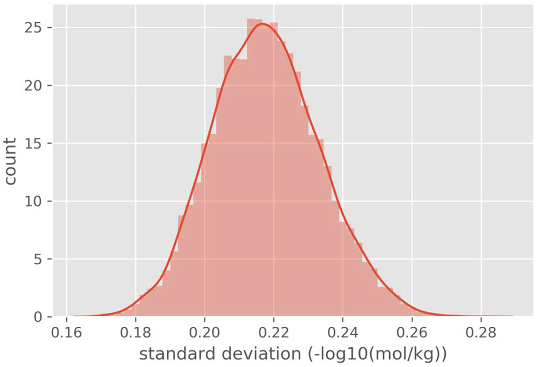
Histogram of the bootstrapped standard deviations.

3.3. Comparison of model predictions to experimental values

To gain an initial understanding of how accurate the predictions from each model were, the chemical-specific residual was compared to the upper 95% confidence value in both the positive and negative directions. Table 2 provides the count and percentage of chemicals with a residual value that was: 1) greater than 0.249 log units, i.e. the model underestimated the in vivo LD50 beyond the experimental variability; 2) within ±0.249 log units, i.e. the model estimated the in vivo LD50 within the experimental variability, and; 3) below −0.249 log units, i.e. the model overestimated the in vivo LD50 beyond the experimental variability.

Table 2.

Counts and percentage of chemicals with residual values relative to the 95% CI threshold

	TEST	TIMES
Above 95% CI threshold	555 (34.2%)	171 (33.9%)
Within the 95% CI threshold	588 (36.3%)	191 (37.9%)
Below the 95% CI threshold	476 (29.4%)	141 (28.0%)

Note: values represent the number of chemicals followed by the percent of total predictions in parentheses.

The predictions for both models are similarly split between being within the 95% confidence interval of experimental variability or outside of the threshold.

Substances that were particularly poorly predicted for TEST included Emetine dihydrochloride (DTXSID7020558; CASRN 314-42-7) that had a 5 log unit difference: experimental LD50 0.012 mg/kg (pLD50 7.66) cf. TEST predicted 2204 mg/kg (pLD50 2.4). Substances that were particularly poorly predicted for TIMES included Echothiophate (DTXSID1022976; CASRN 513-10-0), whose experimental LD50 was 0.174 mg/kg but whose TIMES prediction was 889 mg/kg (experimental pLD50 of 6.34 vs predicted value of 3.35), as well as Butane-1,4-diyl bis(2-methylprop-2-enoate) (DTXSID4044870; CASRN 2081-81-7): experimental LD50 10.07 mg/kg (pLD50 4.35) cf. TIMES 8410 mg/kg ( pLD50 1.42).

Another way to investigate the two models was to generate scatterplots comparing the experimental pLD50s against the predicted pLD50s for TEST and TIMES (Figures 4a and 4b, respectively).

Figure 4a.

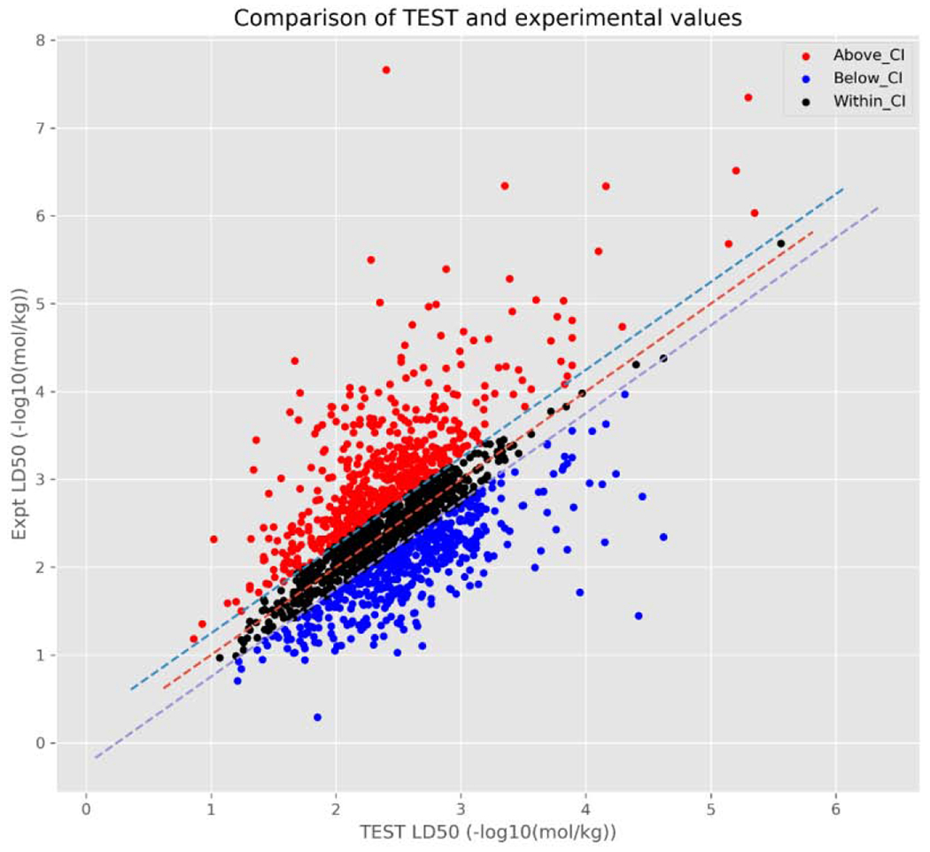
Scatterplot relating TEST predictions vs. actual experimental pLD50 values.

Figure 4b.

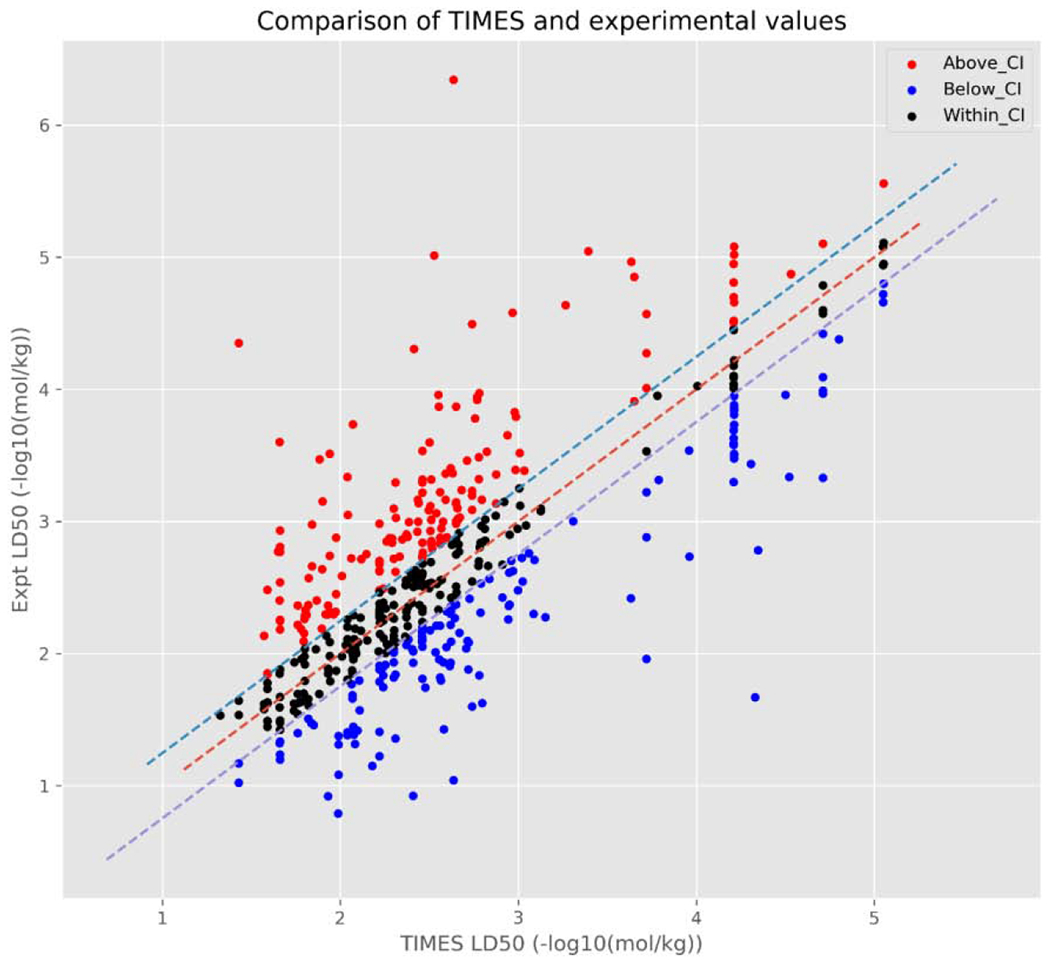
Scatterplot relating TIMES predictions vs. actual experimental pLD50 values.

From these figures, there is a large cluster of chemicals with an experimental pLD50 between 1 and 4 [−log10(mol/kg)] and a predicted pLD50 between 1.5 and 3.5 −log10(mol/kg). Additionally, these figures also highlight the differences in how predictions are derived between the 2 models. The TEST predictions (Figure 4a), are reasonably randomly distributed around the line of zero variance (dashed red line) with no discernible pattern. This is likely to be expected given that the predictions made by TEST utilised in this study are the consensus predictions from up to three separate QSAR models.

On the other hand, the TIMES predictions (Figure 4b) appear to be a combination of randomly distributed points and some discernible patterns, i.e. vertical lines. Again, this is a product of how TIMES makes predictions; whereby, a chemical is first assigned to a toxicological category and the associated QSAR is used to make an LD50 prediction. These toxicological categories fall into one of three types of toxicity: 1) basic toxicity (also called narcosis), where a chemical affects basic cell functions, e.g. non-reactive interaction with cell membranes; 2) excess invariable toxicity, where a chemical interacts with a specific cellular structure/process and has a constant toxicity that is independent of physicochemical properties, and; 3) excess bioavailability dependent toxicity, where a chemical interacts with a specific cellular structure/process and the level of toxicity exhibited is determined by certain physicochemical properties.

Whilst individual linear regression models were derived for the categories comprising excess bioavailability dependent toxicity (explaining the randomly distributed points), none of the models for either basic toxicity or excess invariable toxicity contain an explanatory variable. As such, all chemicals assigned to the same toxicological category within one of these two toxicity types are predicted to have the same pLD50 (± confidence) in −log10(mol/kg). For example, chemicals assigned to the isocyanate excess invariable toxicity category will be predicted to have an pLD50 of 1.82 (±0.15) −log10(mol/kg). It appears this is the reason for the linear patterns throughout Figure 2b, which are best exemplified by chemicals with higher predicted LD50s: here, three vertical lines can be easily distinguished.

Upon further investigation, each line represents a different excess invariable TIMES toxicity category (trifluoromethylbenzimidazoles, organophosphate excess toxicity, and trifluoromethyl tetrahalobenzimidazoles) with all chemicals assigned to the same category being predicted to have the same LD50 by TIMES models. However, the experimental values can vary by up to 2 log units across the chemicals associated with these categories, thus, producing the vertical lines. Assigning all chemicals in the same toxicological category, the same LD50 is a limitation of the TIMES model and should be kept in consideration when a chemical is classified as exhibiting either basic or excess invariable toxicity.

Furthermore, the residuals of chemicals with an over-prediction of pLD50 relative to the representative experimental value have a tendency to be smaller than the residuals of chemicals with an under-prediction of pLD50 relative to the representative experimental value for both models. This can, perhaps, be best observed in Figures 5a and 5b; whereby, chemicals with a predicted pLD50 that overestimates the experimental pLD50 (i.e. a negative residual), generally, have smaller residuals than the underestimated predictions (i.e. a positive residual). This is especially true for those chemicals with a prediction below approximately 3.5 −log10(mol/kg). This appears to be more pronounced for the TEST predictions than the TIMES predictions; although, this may partially be due to TEST making more predictions than TIMES. After further examination of the residuals, predictions made by both models are heteroscedastic (Figures 5a and 5b), i.e. the variance in the residuals increases for chemicals predicted to be of either very high or low toxicity. Again, this was more readily apparent for the TEST predictions; however, this may also be due to the limited number of chemicals TEST predicted with very high toxicity (i.e. above 4.5/5 - log10(mol/kg)).

Figure 5a.

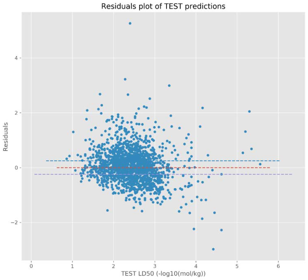
Residuals plot for TEST model predictions.

Figure 5b.

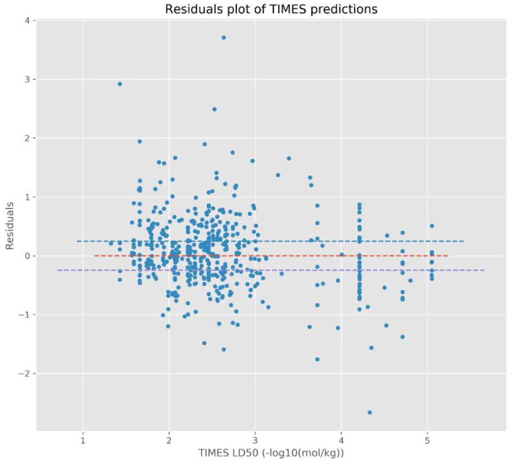
Residual plot for the TIMES model predictions.

There were 58 chemicals with a TIMES prediction above 4 −log10(mol/kg), 16 (27.5%) of which were within the 95% confidence interval of the in vivo variability and 29 (50%) chemicals were below the CI: hence, more conservative in their LD50 estimates. TEST does comparatively worse above this threshold, with 3 of the 20 chemicals (15%) having a prediction within the 95% confidence interval of the in vivo variability but 10 (50%) chemicals being below the CI threshold. Therefore, even though each chemical assigned to one of these categories by TIMES is predicted to have the same LD50, the prediction itself is more likely to be close to, or more conservative than, the experimental value.

To further assess the performance of TEST and TIMES predictions, four performance metrics were computed using all predictions generated by each model, respectively: the root mean square error (RMSE), the mean absolute error (MAE), the coefficient of determination (R²), and the Pearson correlation coefficient. As can be seen in Table 3, the RMSE and MAE for all TEST predictions (0.642 and 0.469 −log10(mol/kg), respectively) are comparable to the RMSE and MAE for all TIMES predictions (0.62 and 0.447 - log10(mol/kg), respectively).

Table 3.

Performance metrics for the TEST (1619 substances) and TIMES (503 substances) models for the respective entire datasets

	TEST	TIMES
RMSE	0.642	0.62
R2	0.296	0.54
MAE	0.469	0.447

Whilst the RMSE and MAE are similar between the two software, the R² values are not, with the TIMES predictions having a much larger R² (0.54) and, therefore, fitting the experimental data much better than the TEST predictions (0.296).

This is also borne out when comparing the correlation coefficients of the two software (Figure 6); whereby, the predictions from both software are positively correlated with the experimental pLD50 values, but the predictions from TIMES have a higher correlation (0.75) than do the TEST predictions (0.57). The higher R² and correlation coefficients observed for the TIMES predictions are likely being driven by the predictions made for the higher potency chemicals, e.g. pLD50 values predicted above 4 (−log10(mol/kg)), such as chemicals assigned to the trifluoromethylbenzimidazole, organophosphate excess toxicity, or trifluoromethyl tetrahalobenzimidazole categories.

Figure 6.

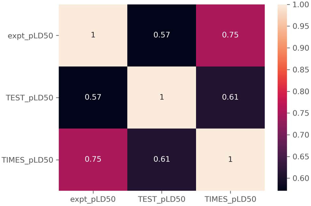
Correlation coefficients for TEST and TIMES relative to experimental pLD50 values.

3.4. Comparison of chemicals with predictions in both TEST and TIMES

After investigating the performance of each software across all chemicals for which a prediction could be made, the chemical list was filtered to include only those chemicals with a LD50 prediction in both the TEST and TIMES models (i.e. the overlap set). Upon applying this additional filtering criteria, a total of 274 chemicals were retained; thus, enabling a comparison of the performance of the two models for the set of chemicals.

For each model, the overall count and percentage of overlapping chemicals show a similar split to the complete subsets of chemicals, with the majority of chemicals having a residual that is within the 95% confidence interval of the in vivo variability (Table 4). TEST, has a slightly greater percentage of chemicals present within this category (40.5%) than does TIMES (38.32%); however, both models have a marginal improvement for the overlap subset compared to the complete subset of chemicals with a prediction.

Table 4.

Counts and percentage of chemicals with residual values relative to the 95% CI threshold for the overlap set

	TEST	TIMES
Above 95% CI threshold	87 (31.8%)	99 (36.1%)
Within the 95% CI threshold	111 (40.5%)	105 (38.3%)
Below the 95% CI threshold	76 (27.7%)	70 (25.5%)

Note: values represent chemical counts followed by percentage of the overlap set in parentheses.

A similar trend is observed when the RMSE and MAE values are compared as both of these metrics stay relatively consistent, with only marginal changes occurring between the complete and overlapping subsets (Table 5). Much larger changes are observed between the TIMES complete and overlap subsets in terms of the R² and correlation coefficients (Figure 7). The R² for the TIMES predictions of the overlapping subset (0.255) is almost half that of the complete subset (0.54) and the correlation coefficient decreases by approximately 0.20 points from 0.75 to 0.56.

Table 5.

Performance metrics for the TEST and TIMES models for the overlap dataset

	TEST	TIMES
RMSE	0.643	0.65
R2	0.27	0.255
MAE	0.457	0.457

Figure 7.

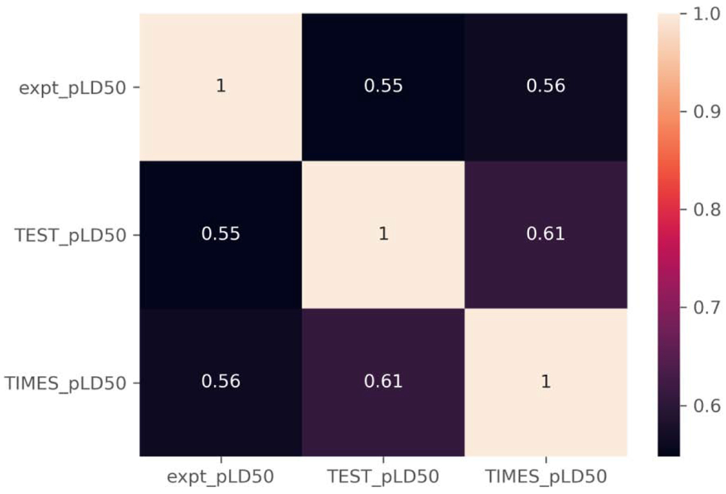
Correlation coefficients for TEST, TIMES relative to experimental pLD50 values for the overlap set.

The decrease in these metrics brings them more in-line with the corresponding metric for the TEST predictions, which remain consistent between the complete and overlap subsets. The differences in the R² and correlation coefficients between the two subsets for the TIMES predictions is likely due to 52 of the 58 higher potency chemicals not being present in the overlap subset, including all of the chemicals in the trifluoromethylbenzimidazole, organophosphate excess toxicity, and trifluoromethyl tetrahalobenzimidazole categories.

3.5. Chemotypes associated with predictions outside confidence intervals

To identify chemical features that may contribute to less accurate predictions of rat oral acute LD50, odds ratios were computed to identify ToxPrints that were more highly enriched in the chemicals having predictions outside of the 95% CI. Only a handful of ToxPrints were enriched with different ToxPrints identified between the models, i.e. the sorts of chemicals that were likely to give rise to less accurate predictions with residuals outside the threshold of variability were different for TEST vs. TIMES (Table 6). The 95% confidence intervals of the odds ratios are shown too to highlight the uncertainties associated with the odds ratios themselves. Some enriched ToxPrints e.g. ring:hetero_[6_6]_O_benzopyrone_(1_4-) are far more uncertain with a much wider confidence interval than others. Due to the hierarchical nature of the ToxPrints themselves, some substances drove the enrichment of multiple ToxPrints e.g. bond:S(=O)N_sulfonylamide and bond:S(=O)N_sulfonamide (Table 7 highlights specific substances). In other circumstances, multiple ToxPrints may be enriched because there is somewhat of an overlap in the structural fragment(s) the ToxPrints code for. For example, of the substances with a TEST prediction outside the 95% CI that contain the ring:hetero_[6_6]_O_benzopyrone_(1_4-) ToxPrint, all but 5 also contain the bond:CC(=O)C_ketone_alkene_cyclic_2-en-1-one ToxPrint. In these instances, it may be difficult to ascertain exactly which of the ToxPrints is driving the enrichment. However, there are an additional 10 substances containing the bond:CC(=O)C_ketone_alkene_cyclic_2-en-1-one ToxPrint with a prediction outside the CI that do not also contain the ring:hetero_[6_6]_O_benzopyrone_(1_4-) ToxPrint. Therefore, it appears that in this study, chemicals containing one or other of these ToxPrints may be more likely to be poorly predicted. Furthermore, some ToxPrints are always present in chemicals with predictions outside the CI. For example, bond:COC_ether_alkenyl and bond:COH_alcohol_allyl identified for TIMES had an odds ratio of “Inf” meaning that none of the chemicals (Table 8) containing those ToxPrints had a prediction that was within the 95% CI. There were no ToxPrints in common between those enriched for presence in low accuracy predictions from TEST vs. TIMES, further highlighting the difference in the training sets and thus applicability domains for the models.

Table 6.

Enriched ToxPrints for TEST and TIMES predictions outside of the threshold of variability

	OR	p-value	TxP	TP	Upper_95%CI	Lower_95%CI
TEST	2.57	0.03	bond:CC(=O)C_ketone_alkene_cyclic_2-en-1-one	31.00	1.13	5.88
	4.25	0.01	bond:S(=O)N_sulfonamide	22.00	1.27	14.27
	4.38	0.00	bond:S~N_generic	30.00	1.53	12.48
	5.04	0.00	bond:S(=O)N_sulfonylamide	26.00	1.52	16.74
	12.20	0.00	ring:hetero_[6_6]_O_benzopyrone_(1_4-)	21.00	1.64	90.97
TIMES	3.28	0.01	bond:quatN_alkyl_acyclic	30	1.34	8.04
	3.52	0.00	bond:quatN_generic	32	1.44	8.59
	4.06	0.02	bond:quatN_trimethyl_alkyl_acyclic	19	1.86	13.92
	6.94	0.04	group:ligand_path_5-7_bidentate	11	0.89	54.22
	inf	0.02	bond:COC_ether_alkenyl	9	-	-
	inf	0.03	bond:COH_alcohol_allyl	8	-	-

OR = Odds Ratio, TxP = ToxPrint fingerprint, TP = Number of True Positives, Upper(Lower) 95% CI = Upper(Lower) 95% Confidence interval of the Odds Ratio

Table 7.

TEST substances that contain bond:S(=O)N_sulfonamide or bond:S(=O)N_sulfonylamide

DTXSID	Name	known_LD50_mg kg	TEST_LD50_mg kg	TEST
DTXSID6049016	Sematilide monohydrochloride	3200	494.2045107	Below_CI
DTXSID1045615	Fasudil hydrochloride	335	1275.406699	Above_CI
DTXSID2046628	Tamsulosin hydrochloride	650	2230.132833	Above_CI
DTXSID6032645	Sulfentrazone	2855	476.3354627	Below_CI
DTXSID30179415	4-Hydroxy-2-methyl-2H-1,2-benzothiazine-3-carboxylic acid ethylester 1,1-dioxide	4800	1294.930841	Below_CI
DTXSID5067182	Benzenesulfonamide, 4-amino-2,5-dichloro-N,N-dimethyl-	4087	1380.315129	Below_CI
DTXSID50187653	Sudoxicam	136	68.88211304	Below_CI
DTXSID2057601	Glymidine sodium	2850	6764.686158	Above_CI
DTXSID5021170	Piroxicam	216	1779.454857	Above_CI
DTXSID7048611	1-[2-({[5-Diethylamino)-2-{[4-(dimethylsulfamoyl)phenyl]diazenyl}phenyl]sulfonyl}amino)ethyl]pyridinium chloride	5125	1186.556007	Below_CI
DTXSID1068487	Hexanoic acid, 6-[methyl(phenylsulfonyl)amino]-	3040	1680.324255	Below_CI
DTXSID0068496	Benzenesulfonamide, 4-amino-5-methoxy-N,2-dimethyl-	91.5	1871.786113	Above_CI
DTXSID2068507	Benzenesulfonamide, 4-amino-2,5-dimethoxy-N-methyl-	815	1703.841315	Above_CI
DTXSID8045486	Tenoxicam	79	23.34030147	Below_CI
DTXSID00976211	N-[4-(N,N-Diethylalanyl)phenyl]methanesulfonamide--hydrogen chloride (1/1)	2347	943.7637084	Below_CI
DTXSID6046133	Lornoxicam	5.73	47.89840658	Above_CI
DTXSID7026499	4,4′-Oxybis(benzenesulfohydrazide)	2300	1082.320497	Below_CI
DTXSID5021251	Saccharin	14200	1670.621456	Below_CI
DTXSID8023470	Phthalylsulfathiazole	2001	327.9202151	Below_CI
DTXSID9034868	Prosulfuron	986	4005.047907	Above_CI
DTXSID8021278	Sotalol hydrochloride	3450	1046.418523	Below_CI
DTXSID20877236	N-(4-chlorobenzene-1-sulfonyl)-N′-cyclohexylcarbamimidic acid	1525	4176.237348	Above_CI

Table 8.

TIMES substances with ToxPrints with an odds ratio of ‘inf’

DTXSID	Name	known_LD50_mgkg	TIMES_LD50_mgkg	TIMES
DTXSID20182958	Flavoxate succinate	1445	482	Below_CI
DTXSID1047784	Flavoxate hydrochloride	1040	482	Below_CI
DTXSID20958998	8-[(Dimethylamino)methyl]-7-methoxy-2,3-dimethyl-4H-1-benzopyran-4-one--hydrogenchloride (1/1)	7.8	321	Above_CI
DTXSID3047847	Nalorphine hydrochloride	1150	349	Below_CI
DTXSID2022830	Clavulanic acid	7936	3460	Below_CI
DTXSID20207074	4H-1-Benzopyran-8-carboxylic acid, 3-methyl-4-oxo-2-phenyl-, sodium salt	1655	345	Below_CI
DTXSID90208992	Phosphoric acid, bis(2-methylpropyl) 1,6-dihydro-5-methoxy-1-methyl-6-oxo-4-pyridazinyl ester	36	6.52	Below_CI
DTXSID60210067	Clavulanate potassium	7936	3460	Below_CI
DTXSID30223048	4H-1-Benzopyran-6-carboxylic acid, 3-isopropoxy-2-(p-methoxyphenyl)-4-oxo-,sodium salt	1480	5120	Above_CI
DTXSID2040363	Diniconazole	474	898	Above_CI
DTXSID3035002	Uniconazole-P	430	804	Above_CI
DTXSID2034548	Diniconazole-M	474	898	Above_CI
DTXSID7032505	Uniconazole	1790	804	Below_CI
DTXSID2040363	Diniconazole	474	898	Above_CI
DTXSID30235540	Terflavoxate hydrochloride	1977	516	Below_CI

Table 9 showcases a handful of examples where the probability of a ToxPrint being present for substances that fell outside of the confidence interval was computed for both models and the ratio taken. This was intended to provide an indication of which model was preferable to use for a given substance depending on the ToxPrints it contained. As an example, the set of 32 ToxPrints for DTXSID20182958 [CASRn 28782-19-6] Flavoxate succinate was identified. The product of the probabilities for each model (equating the probability of all 32 ToxPrints being present) was computed. For TEST, this equated to 1.72E-32 and for TIMES, 1.219E-34. The ratio of these two probabilities was defined as the confidence metric which is calculated to be 141.15, suggesting that TEST is the preferred model to use in this case.

Table 9.

Example substances with computed ToxPrint probabilities calculated to illustrate model selection based on presence of ToxPrint chemical features outside of the confidence interval range

Substance ID	Name	Known LD50 mg/kg	TEST LD50 mg/kg	TIMES LD50 mg/kg	Confidence index(TEST:TIMES)	Comments
DTXSID3025461	Isobutyl methacrylate	9590	3490	5280	0.3	TIMES model favoured for prediction
DTXSID20182958	Flavoxate succinate	1445	509	482	141	TEST model favoured for prediction
DTXSID1030319	3-amino-9-ethylcarbazole	144	620	540	0.08	TIMES model favoured for prediction

Conclusions

Acute oral systemic toxicity is an endpoint that is required for a number of different regulatory contexts. Here a large body of rat acute oral toxicity data was utilised to evaluate the performance of LD50 models within two expert systems: TEST and TIMES. To benchmark the performance of the models, predictions were only considered for chemicals that were not part of the training sets for each model, respectively. The relative performance was compared to a 95% CI threshold established by bootstrapping the standard deviation across experimental data for chemicals with at least three LD50 values. Given the upper 95% CI was rather small, many of the predictions derived lay outside of this threshold range. Past evaluations of variability are limited to the variability study conducted by Hoffman et al [20] as part of the EU AcuteTox project which reported a median log transformed standard deviation of ~0.2 for rat and mouse acute oral toxicity studies and appears similar to the mean of the bootstrapped replicates of standard deviations found here, 0.218 though in units of −log10(mol/kg).

TEST was able to make predictions for more chemicals relative to TIMES and the performance characteristics in terms of the RMSE and MAE values were similar between the two models, (TEST: RMSE 0.642, MAE 0.469; TIMES RMSE 0.62, MAE 0.447). The coefficient of determination of TIMES was much higher (0.54) than that for TEST (0.296), but this value decreased (0.27-2.55) when the assessment was limited to chemicals for which both models generated predictions. ToxPrints that were enriched were identified for chemicals that fell outside the upper 95% CI for both TEST and TIMES. These enriched ToxPrints were different for the 2 models indicating that the least robust predictions for the TIMES and TEST models, in terms of the highest residual values, were for different types of chemicals, highlighting differences in the models’ strengths likely due to different training sets and ultimately different domains of applicability. A confidence metric was proposed as a means to aid selection of models for substances outside of this 95% CI on the basis of ToxPrints. Further it is worth noting, that the evaluation was impacted by the extent to which the training set of the 2 models overlapped with the reference set, limiting the number of chemicals for which the performance assessment could be undertaken. This was particularly evident for the TEST model which had a large overlap between its training set and the reference set. TEST and TIMES were developed in very different ways with comparable performance for chemicals for which both models generated predictions, and a slightly better performance from TIMES when considering their performance separately. This highlights the benefits of combining models together to leverage their respective strengths.

The evaluation was informative in terms of highlighting the potential that structure-based models have in predicting acute oral toxicity. The release of the dataset compiled has prompted many subsequent models to be developed, examples of newer studies include new k-nn approaches by Alberga et al [21], various SAR and QSAR approaches by Gadaleta et al [22] as well as read-across approaches such as Helman et al [23] and those incorporating mechanistic information from in vitro high throughput screening assays by Russo et al [24], This analysis also reinforces the benefits of developing a large collaborative modelling project that takes advantage of all the data collected to develop new refined models, such as those captured in the ongoing work in developing the CATMOS suite that exploited the relative strengths and limitations of the different models derived as part of the global international modelling project (see https://ntp.niehs.nih.gov/whatwestudy/niceatm/3rs-meetings/past-meetings/tox-models-2018/index.html) and https://github.com/NIEHS/OPERA/releases which contains the CATMOS models themselves. As noted in Table 10, the availability of this dataset has resulted in an improvement in the performance of acute oral toxicity LD50 models.

Table 10.

Performance metrics for selected models.

Model	R2	RMSE	MSE	Approach
TIMES [16]	0.85		0.15	Expert system
TIMES (in this study)	0.54	0.62		Expert system
TEST [15]	0.626	0.594		Consenus model of 3 local approaches
TEST (in this study)	0.296	0.642		Consenus model of 3 local approaches
Alberga [21]	0.737	0.408		k-NN
Gadaleta [22]	0.59-0.651	0.541-0.585		Various
CATMOS	0.65	0.49		Consensus

Highlights.

• TEST and TIMES acute oral LD50 models were similar in performance.

• TEST was able to make predictions for more chemicals than TIMES (3927 vs 863).

• Poorly predicted substances were different between the models.

References

- [1].Strickland J, Clippinger AJ, Brown J, et al. Status of acute systemic toxicity testing requirements and data uses by U.S. regulatory agencies. Regul Toxicol Pharmacol. 94 (2018) 183–196. doi: 10.1016/j.yrtph.2018.01.022 [DOI] [PMC free article] [PubMed] [Google Scholar]
- [2].Walum E Acute oral toxicity. Environ Health Perspect. 106 (1998) 497–503. doi: 10.1289/ehp.98106497 [DOI] [PMC free article] [PubMed] [Google Scholar]
- [3].Corvaro M, Gehen S, Andrews K, Chatfield R, Arasti C, Mehta J GHS additivity formula: A true replacement method for acute systemic toxicity testing of agrochemical formulations. Regul Toxicol Pharmacol. 82 (2016) 99–110. doi: 10.1016/j.yrtph.2016.10.007 [DOI] [PubMed] [Google Scholar]
- [4].Kinsner-Ovaskainen A, Bulgheroni A, Hartung T, Prieto P ECVAM’s ongoing activities in the area of acute oral toxicity. Toxicol In Vitro. 23 (2009) 1535–1540. doi: 10.1016/j.tiv.2009.07.004 [DOI] [PubMed] [Google Scholar]
- [5].Kleinstreuer NC, Karmaus A, Mansouri K, Allen DG, Fitzpatrick JM, Patlewicz G Predictive Models for Acute Oral Systemic Toxicity: A Workshop to Bridge the Gap from Research to Regulation. Comput Toxicol. 8 (2018) 21–24. doi: 10.1016/j.comtox.2018.08.002 [DOI] [PMC free article] [PubMed] [Google Scholar]
- [6].Enslein K, Lander TR, Tomb ME, Craig PN A predictive model for estimating rat oral LD50 values. Toxicol. Ind.Health 5 (1989) 265–265. [DOI] [PubMed] [Google Scholar]
- [7].Bhogal N, Grindon C, Combes R, Balls M Toxicity testing: creating a revolution based on new technologies. Trends Biotechnol 23 (2005) 299–307. doi: 10.1016/j.tibtech.2005.04.006 [DOI] [PubMed] [Google Scholar]
- [8].Advanced Chemistry Development, Inc., Toronto, ON, Canada. [Google Scholar]
- [9].MultiCASE Inc. http://www.multicase.com/
- [10].Schultz TW, Diderich R, Kuseva CD, Mekenyan OG The OECD QSAR Toolbox Starts Its Second Decade. Methods Mol Biol. 1800 (2018) 55–77. doi: 10.1007/978-1-4939-7899-1_2 [DOI] [PubMed] [Google Scholar]
- [11].Martin TM, Lilavois CR, Barron MG Prediction of pesticide acute toxicity using two-dimensional chemical descriptors and target species classification. SAR QSAR Environ Res. 2017;28(6):525–539. doi: 10.1080/1062936X.2017.1343204 [DOI] [PMC free article] [PubMed] [Google Scholar]
- [12].Lei T, Li Y, Song Y Li D, Sun H, Hou T. ADMET evaluation in drug discovery: 15. Accurate prediction of rat oral acute toxicity using relevance vector machine and consensus modeling. J Cheminform 8 (2016). 10.1186/s13321-016-0117-7 [DOI] [PMC free article] [PubMed] [Google Scholar]
- [13].Lu J, Peng J, Wang J, Shen Q, Bi Y, Gong L, Zheng M, Luo X, Zhu W, Jiang H, Chen K Estimation of acute oral toxicity in rat using local lazy learning. J Cheminform. 6 (2014) doi: 10.1186/1758-2946-6-26 [DOI] [PMC free article] [PubMed] [Google Scholar]
- [14].Xu Y, Pei J, Lai L Deep Learning Based Regression and Multiclass Models for Acute Oral Toxicity Prediction with Automatic Chemical Feature Extraction. J Chem Inf Model. 57(2017) 2672–2685. doi: 10.1021/acs.jcim.7b00244 [DOI] [PubMed] [Google Scholar]
- [15].Zhu H, Martin TM, Ye L, Sedykh A, Young DM, Tropsha A Quantitative structure-activity relationship modeling of rat acute toxicity by oral exposure. Chem Res Toxicol. 22 (2009) 1913–1921. doi: 10.1021/tx900189p [DOI] [PMC free article] [PubMed] [Google Scholar]
- [16].Nedelcheva D, Stoeva S, Dimitrov S, Detroyer A, Fadli A, Note R, Blanchet D, Mekenyan O In silico mechanistically-based profiling module for acute oral toxicity. Computational Toxicology 12 (2019) 100109. [Google Scholar]
- [17].Williams AJ, Grulke CM, Edwards J, et al. The CompTox Chemistry Dashboard: a community data resource for environmental chemistry. J Cheminform. 9 (2017) 61. doi: 10.1186/s13321-017-0247-6 [DOI] [PMC free article] [PubMed] [Google Scholar]
- [18].Grulke C, Williams AJ, Thillanadarajah I, Richard AM EPA’s DSSTox database: History of development of a curated chemistry resource supporting computational toxicology research. Computat Toxicol 12 (2019) 1000096. [DOI] [PMC free article] [PubMed] [Google Scholar]
- [19].Wang J, Hallinger DR, Murr AS, Buckalew AR, Lougee RR, Richard AM, Laws SC, Stoker TE High-throughput screening and chemotype-enrichment analysis of ToxCast phase II chemicals for human sodium-iodide symporter (NIS) inhibition. Environmental International 126 (2019) 377–386. [DOI] [PMC free article] [PubMed] [Google Scholar]
- [20].Hoffmann S, Kinsner-Ovaskainen A, Prieto P, Mangelsdorf I, Bieler C, Cole T Acute oral toxicity: Variability, reliability, relevance and interspecies comparison of rodent LD50 data from literature surveyed for the ACuteTox project. Regul Toxicol Pharm. 58 (2010) 395–407. [DOI] [PubMed] [Google Scholar]
- [21].Alberga D, Trisciuzzi D, Mansouri K, Mangiatordi GF, Nicolotti O. Prediction of Acute Oral Systemic Toxicity Using a Multifingerprint Similarity Approach. Toxicol Sci, 167 (2019) 484–495. 10.1093/toxsci/kfy255 [DOI] [PubMed] [Google Scholar]
- [22].Gadaleta D, Vukovic K, Toma C Lavado GJ, Karmaus AL, Mansouri K, Kleinstreuer NC, Benfenati E. SAR and QSAR modeling of a large collection of LD50 rat acute oral toxicity data. J Cheminform 11 (2019). 10.1186/s13321-019-0383-2 [DOI] [PMC free article] [PubMed] [Google Scholar]
- [23].Helman G, Shah I, Patlewicz G Transitioning the generalised read-across approach (GenRA) to quantitative predictions: A case study using acute oral toxicity data. Computational Toxicology 12 (2019) 100097. [DOI] [PMC free article] [PubMed] [Google Scholar]
- [24].Russo DP, Strickland J, Karmaus AL, Wang W, Shende S, Hartung T, Aleksuuunes LM, Zhu H Nonanimal Models for Acute Toxicity Evaluations: Applying Data-Driven Profiling and Read-Across. Environ Health Perspect. 127 (2019) 47001. doi: 10.1289/EHP3614 [DOI] [PMC free article] [PubMed] [Google Scholar]