Impact of Adolescent Obesity on Middle-Age Health of Women Given Data MAR

Abstract

We analyze adolescent BMI and middle-age systolic blood pressure (SBP) repeatedly measured on women enrolled in the Fels longitudinal study (FLS) between 1929 and 2010 to address three questions: Do adolescent-specific growth rates in BMI and menarche affect middle-age SBP? Do they moderate the aging effect on middle-age SBP? Have the effects changed over historical time? To address the questions, we propose analyzing a growth curve model (GCM) that controls for age, birth-year cohort and historical time. However, several complications in the data make the GCM analysis non-standard. First, the person-specific adolescent BMI and middle-age SBP trajectories are unobservable. Second, missing data are substantial on BMI, SBP and menarche. Finally, modeling the latent trajectories for BMI and SBP, repeatedly measured on two distinct sets of unbalanced time points, are computationally intensive. We adopt a bivariate GCM for BMI and SBP with correlated random coefficients. To efficiently handle missing values of BMI, SBP and menarche assumed missing at random, we estimate their joint distribution by maximum likelihood via the EM algorithm where the correlated random coefficients and menarche are multivariate normal. The estimated distribution will be transformed to the desired GCM for SBP that includes the random coefficients of BMI and menarche as covariates. We demonstrate unbiased estimation by simulation. We find that adolescent growth rates in BMI and menarche are positively associated with and moderate the aging effect on SBP in middle age, controlling for age, cohort and historical time, but the effect sizes are at most modest. The aging effect is significant on SBP, controlling for cohort and historical time, but not vice versa.

1. Introduction

The Fels longitudinal study (FLS) collected the lifetime repeated measurements on growth, health and body composition of 2,567 participants enrolled in yearly cohorts of 20 to 35 from 1929 to 2010. The participants were scheduled to be examined every six months for the first 18 years and every two years for the rest of their life spans. Each examination took extensive anthropometric measurements and recorded a health inventory (Sun et al. 2007, 2008). Via a growth curve model (GCM) with person-specific growth trajectories, also known as a hierarchical, multilevel, random coefficients or linear mixed model (Raudenbush and Bryk 2002; Goldstein 2003), we link growth in adolescent BMI and person-specific (age at) menarche to the course of middle-age systolic blood pressure (SBP) for 835 female participants where 459 women were enrolled at birth producing 85% of the repeated measurements while others were family members, spouses and relatives. In this paper, we consider BMI and SBP as the biomarkers of obesity and health, respectively.

Figure 1 plots all observed BMI and SBP of the participants against age where 5,694 adolescent BMIs and 1,196 middle-age SBPs are nested within 552 and 436 individuals, respectively. It superimposes the scatterplots with person-specific longitudinal spaghetti plots. BMI and SBP are standardized to have mean 0 and variance 1. Every participant has at least one observation in adolescence or middle age. The spaghetti plots reveal that some growth patterns in BMI are higher overall, accelerate earlier or decelerate earlier than others. We analyze the impact of the growth patterns on progression of middle-age SBP. Because the 835 female participants consist of 98% European Americans and a tiny fraction of minority participants including African American, Asian, multiracial and other individuals and because the minority effect is not significant on either BMI or SBP outcome in preliminary analysis, we do not consider the race covariate.

Figure 1:

Scatter and spaghetti plots superimposed for the unbalanced repeated measurements of adolescent BMI and middle-age SBP against age from 835 FLS female participants enrolled over time across multiple birth year cohorts.

The examination schedule implies that those enrolled at age 10 or earlier can have up to 18 adolescent measurements between 10 and 19 years of age and up to 10 middle-age measurements between 45 and 65 years of age, depending on how old they are as of 2010. Some relatives, spouses and family members of the participants enrolled in the FLS during adolescence or later produced their measurements afterward. It is, however, unreasonable to take all these repeated measurements as complete data for analysis because only 18% of the 835 participants have at least one measurement in both adolescence and middle age. Instead, we realistically take the measurements at the time points of actual visits to a clinic for examination and menarche as complete data and assume data missing at random (MAR, Rubin 1976). As the spaghetti plots in Figure 1 show, the actual timings of examinations varied, and BMI appears semi-regularly measured while SBP looks more sparse and unbalanced.

Family relocations due to job transfers or newly acquired jobs, sickness of participants or family members accompanied to scheduled examinations, or other family emergencies or situations may have caused participants to miss scheduled examinations or attrite. During the scheduled examinations, 12% of the adolescents and 18% of adults failed to have their BMI and SBP measured, respectively, for some reasons. Menarche was either identified at a scheduled examination or obtained from participants’ recollections, but missing otherwise. It seems plausible that the missing patterns are not related to missing values themselves. As a reviewer pointed out, however, it is possible for an adolescent to have a high BMI worsened since the last examination and fail to participate in the next scheduled examination because of embarrassment or anxiety. As the reviewer also commented, participants who have adolescent BMI measurements but who have no SBP measurement as adults are likely to be unhealthy and have high SBP in middle age. The missing BMI and SBP will be associated with missing probability to violate the MAR assumption. However, because the missing rates on BMI and SBP are modest, because 40% of the female participants having adolescent BMI measurements are younger than middle age as of 2010, and because most adolescents appear to have attended most follow-ups in the spaghetti plots, even if some missing BMI and SBP are NMAR, they will not seriously affect our analysis.

We leverage the FLS data collected longitudinally on individuals enrolled over time to estimate the age, cohort and historical time effects separately. In large-scale single cohort studies such as the Dunedin Longitudinal Study and the Environmental-Risk Longitudinal Twin Study (Caspi et al. 2016; Moffitt et al. 2011), age and historical time are perfectly correlated. The confounded effects of age and childhood factors may explain only modest effect sizes of childhood risk factors on adult health outcomes reported (Felitti et al. 1998; Roberts et al. 2007; Moffitt et al. 2011; Caspi et al. 2016). On the contrary, age and cohort are perfectly collinear in a cross-sectional study of multiple birth year cohorts such as National Growth and Health Studies (Ren and Shin 2016). The multi-cohort FLS enables us to control for temporal, cohort and historical sources of SBP, and estimate the main effects of growth rates in adolescent BMI and menarche, and the growth rates-by-age and menarche-by-age interaction effects on middle-age SBP by a multilevel GCM. These effects may also change over cohorts and time.

Researchers have studied the impact of longitudinal growth patterns in childhood obesity on adult health or the effects of childhood covariates on a longitudinal adult outcome in linear and nonlinear mixed models (Eriksson et al. 1999; Law et al. 2002; Ferreira et al. 2005; Nooyens et al. 2007; Sabo et al. 2012; McLeod et al. 2018; Sabo et al. 2014). Kim et al. (2016) analyzed FLS longitudinal childhood BMI to predict the person-specific timing of the BMI rebound, and subsequently analyzed the impact of the timing on a longitudinal adult cardiac outcome. Sabo et al. (2017) analyzed the FLS childhood BMI to predict child-specific ages and BMIs at the BMI rebound and maximum BMI growth, and subsequently estimated the effects of the predicted childhood covariates on longitudinal adulthood blood pressure outcomes. These studies have assessed the impact of either adult characteristics on a longitudinal childhood outcome or childhood covariates on a longitudinal adult outcome.

In structural equation models (Bollen 1989), a longitudinal model for the repeated measurements of an outcome nested within individuals may be efficiently estimated by latent growth modeling where age variables are considered as fixed factor loadings and random coefficients are latent variables (Willett and Sayer 1994; MacCallum et al. 1997; Bauer 2003; Bollen and Curan 2006; Preacher et al. 2008; Grimm and Ram 2009; Ram and Grimm 2015). Growth-mixture modeling extends the latent growth model to identify unobserved subpopulations exhibiting different growth trajectories (Wang and Bodner 2007). These approaches model longitudinal outcomes measured on a common set of time points.

In the joint modeling approach (Gueorguieva 2001; Ivanova et al. 2016), a mixture of discrete and continuous longitudinal outcomes may be modeled in a joint mixed model. Data MAR in the model may be imputed by univariate sequential regression models (Raghunathan et al. 2001), also known as multiple imputation by fully conditional specification (van Buuren et al. 2006; van Buuren 2011). A multilevel GCM given data MAR may also be efficiently estimated by maximum likelihood (ML) or Bayesian methods (Liu et al. 2000; Schafer and Yucel 2002; Goldstein and Browne 2002; Goldstein et al. 2009; Goldstein and Kounali 2009; Shin and Raudenbush 2007, 2010, 2020; Ren and Shin 2016). These approaches typically apply to longitudinal outcomes measured at a common set of time points.

In this paper, we estimate a nonstandard multilevel GCM for middle-age SBP that introduces challenges. First, the key covariates are unobservable adolescent-specific growth rates in BMI that have to be estimated from sample data. Sample average growth rates, for example, are unreliable measurements of the true growth rates that are known to introduce bias in the estimated effects of the growth rates (Lüdtke et al. 2008; Shin and Raudenbush 2010, 2020; Grilli and Rampichini 2011). Furthermore, missing data are substantial on BMI, SBP and menarche. Finally, longitudinal m_j BMIs in adolescence and n_j SBPs in middle age are measured at two separate sets of unbalanced time points nested within each person, and subjects may have measurements in either adolescence or middle age, or both. To handle missing data efficiently, we may express, as a special case of the joint modeling approach, a bivariate multilevel GCM for BMI and SBP and a linear model for menarche jointly where correlated person-specific random coefficients and menarche are multivariate normal and the variance covariance structure is appropriately constrained. Computationally efficient estimation of the joint model, however, involves derivation of new estimators and considerable amount of programming in a way that fully leverage the longitudinal structure. Our method is tailored to the structure with one set of outcomes repeatedly measured at unbalanced time points during childhood and another set longitudinally measured at separate unbalanced time points as an adult within each individual, thereby achieving computational efficiency.

Viewing BMI, SBP, menarche and random coefficients as complete data, we analyze all observed data to estimate the joint model efficiently by ML via the EM algorithm (Dempster et al. 1977; Dempster et al. 1981; Shin and Raudenbush 2007). At convergence, we compute standard errors by the approximate Fisher score (Hedeker and Gibbons 1994; Raudenbush et al. 2000; Olsen and Schafer 2001). Subsequently, by the delta method (Casella and Berger 2002), we transform the estimated joint model to the desired GCM for SBP that includes the random coefficients of adolescent BMI and menarche as covariates. An alternative is to draw multiple imputation of completed data, including the random coefficients, from the estimated joint model and estimate the desired GCM given the multiple imputation (Shin and Raudenbush 2007). This approach requires a cumbersome extra step of multiple imputation. We choose the delta method that demanded less programming than the alternative. We will demonstrate unbiased estimation by simulation. Our findings may provide important policy implications to promote adult health based on juvenile obesity history.

Although FLS has not selected participants with respect to factors known to be associated with body composition, health, and other related conditions (Roche 1992), the participants are far from being randomly assigned to levels of key covariates, BMI growth rates and menarche. Furthermore, with adolescence far apart from middle age in time, there can be a number of confounders of the key covariates that we have not considered such as socioeconomic and environmental covariates unavailable in FLS. Consequently, the effect we mention in this paper is associational, not causal.

The Fels data set is not publically available. However, the data set analyzed in this paper will be available from the second author upon reasonable request. The next section introduces our model. Section 3 explains how to estimate the model and compute standard errors given data MAR. Section 4 evaluates the accuracy and precision of the estimation by simulation. Section 5 presents analysis of the multi-cohort FLS sample data. The final section discusses the limitations and future extensions of the approach.

2. Model

Following Raudenbush and Bryk (2002), we express the repeated measurements of middle-age SBP R_ij and adolescent BMI C_tj for adult occasion i and adolescent occasion t within person j in a level-1 model

$$R_{ij}=A_{Rij}^T{\beta }_{Rj}+B_{Rij}^T{\gamma }_{R1}+{ϵ}_{Rij},\hspace{1em}{ϵ}_{Rij}~N\left(0,{\sigma }_{RR}\right),$$ (1)

$$C_{tj}=A_{Ctj}^T{\beta }_{Cj}+B_{Ctj}^T{\gamma }_{C1}+{ϵ}_{Ctj},\hspace{1em}{ϵ}_{Ctj}~N\left(0,{\sigma }_{CC}\right)$$ (2)

where $A_{Rij}^T{\beta }_{Rj}$ is a polynomial in adult age a_ij for vectors A_Rij of age terms and β_Rj of person-specific age effects (e.g. $A_{Rij}^T=\left[\begin{array}{cc}1& a_{ij}\end{array}\right]$ and ${\beta }_{Rj}^T=\left[\begin{array}{cc}{\beta }_{R0j}& {\beta }_{R1j}\end{array}\right]$), B_Rij is a vector of known covariates (e.g. historical time) having fixed effects γ_R1, $A_{Ctj}^T{\beta }_{Cj}$ is a polynomial in adolescent age a_tj for vectors A_Ctj of age terms and β_Cj of adolescent-specific age effects (e.g. $A_{Ctj}^T=\left[\begin{array}{ccc}1& a_{tj}& a_{tj}^2\end{array}\right]$ and ${\beta }_{Cj}^T=\left[\begin{array}{ccc}{\beta }_{C0j}& {\beta }_{C1j}& {\beta }_{C2j}\end{array}\right]$), B_Ctj is a vector of known covariates having fixed effects γ_C1 (e.g. $a_{tj}^3$ and historical time), and occasion-specific random errors ϵ_Rij and ϵ_Ctj are independent for i = 1, ⋯, n_j, t = 1, ⋯, m_j and j = 1, ⋯, J. With adolescence and middle age far apart within each person, it appears reasonable that occasion-specific random errors ϵ_Rij and ϵ_Ctj are uncorrelated given the person-specific growth trajectories β_Rj and β_Cj and time-varying covariates. That is, given the covariates, SBP and BMI are dependent on each other only through the dependence between the trajectories.

The aging effects β_Rj on SBP vary between individuals according to a level-2 model

$${\beta }_{Rj}={\Gamma }_{R0}{U}_j+v_j,\hspace{1em}{v}_j~N\left(0,\tau \right)$$ (3)

for a matrix Γ_R0 of fixed effects; a vector $U_j={\left[\begin{array}{ccc}{W}_{2j}^T& Y_{2j}^T& {\beta }_{Cj}^T\end{array}\right]}^T$ of known covariates W_2j (e.g. cohort), partially observed covariates Y_2j (e.g. menarche) and unobservable growth rates β_Cj in adolescent BMI; and a vector of random effects ν_j independent of random errors and U_j. Conditional on ν_j and covariates, SBP and BMI are independent. Although the growth trajectories may also vary differently across subpopulations to produce non-constant variances of random coefficients, for example, between males and females, we believe that the constant variance covariance matrix τ is plausible within our analysis of females, controlling for U_j. Equations (1) and (3) imply our desired GCM (Raudenbush and Bryk 2002)

$$R_{ij}=A_{Rij}^T{\Gamma }_{R0}{U}_j+B_{Rij}^T{\gamma }_{R1}+A_{Rij}^T{v}_j+{ϵ}_{Rij}$$ (4)

for a matrix of fixed effects Γ_R0 including the effects of aging moderated by U_j, the fixed effects γ_R1 of B_Rij, and the random effects v_j of A_Rij independent of ϵ_Rij.

Estimation of GCM (4) is difficult because (R_ij, C_tj, Y_2j) are partially observed and because latent trajectories β_Cj are unobservable. We introduce efficient and unbiased estimation below. For a positive integer n, let I_n be an n-by-n identity matrix, 1_n be a vector of n unities, a diagonal matrix ${\oplus }_{i=1}^n{A}_i=diag\left\{A_1,\cdots ,A_n\right\}$, probability density function (pdf) f (A) and conditional pdf f (A|B).

3. Efficient Estimation

For efficient estimation by all observed data, we estimate the joint distribution of (R_ij, C_tj, Y_2j) MAR given known covariates. We view q random coefficients ${\beta }_{1j}={\left[\begin{array}{cc}{\beta }_{Rj}^T& {\beta }_{Cj}^T\end{array}\right]}^T$ and p₂ variables Y_2j as level-2 complete data in a model $f\left(Y_{2j}^{\ast }\right)$

$$Y_{2j}^{\ast }=X_{2j}{\gamma }_2+b_j,\hspace{1em}{b}_j~N\left(0,T\left({\varphi }_T\right)\right)$$ (5)

for $Y_{2j}^{\ast }={\left[\begin{array}{cc}{\beta }_{1j}^T& Y_{2j}^T\end{array}\right]}^T$, a matrix of covariates $X_{2j}=diag\left\{X_{21j},X_{22j}\right\}$ having fixed effects ${\gamma }_2=\left[\begin{array}{c}{\gamma }_{21}\\ {\gamma }_{22}\end{array}\right]$, random effects $b_j=\left[\begin{array}{c}{b}_{1j}\\ b_{2j}\end{array}\right]$ and $T\left({\varphi }_T\right)=\left[\begin{array}{cc}{T}_{11}& T_{12}\\ T_{21}& T_{22}\end{array}\right]$ having distinct elements ϕ_T for $X_{21j}=I_q\otimes W_{2j}^T$ and $X_{22j}=I_{p2}\otimes W_{2j}^T$. Each outcome in $Y_{2j}^{\ast }$ may control for a different subset of W_2j as we do in Section 6. Let ${\theta }_2={\left[\begin{array}{cc}{\gamma }_2^T& {\varphi }_T^T\end{array}\right]}^T$.

We aggregate $R_j={\left[\begin{array}{ccc}{R}_{1j}& \cdots & R_{n_{j}j}\end{array}\right]}^T$ and $C_j={\left[\begin{array}{ccc}{C}_{1j}& \cdots & C_{m_{j}j}\end{array}\right]}^T$ to view $Y_{1j}={\left[\begin{array}{cc}{R}_j^T& C_j^T\end{array}\right]}^T$ and $Y_{2j}^{\ast }$ as complete data and observed values of $Y_j={\left[\begin{array}{cc}{Y}_{1j}^T& Y_{2j}^T\end{array}\right]}^T$ as observed data for person j, and estimate the joint model $f\left(Y_{1j},Y_{2j}^{\ast }\right)=f\left(Y_{1j}|{\beta }_{1j}\right)f\left(Y_{2j}^{\ast }\right)$ given known covariates by the EM algorithm. We aggregate Equations (1) and (2) as the level-1 model f (Y_1j|β_1j)

$$Y_{1j}=A_{1j}{\beta }_{1j}+B_{1j}{\gamma }_1+{ϵ}_{1j},\hspace{1em}{ϵ}_{1j}~N\left(0,{\psi }_j\right)$$ (6)

of person j where A_1j = diag{A_Rj, A_Cj}, ${\beta }_{1j}={\left[\begin{array}{cc}{\beta }_{Rj}^T& {\beta }_{Cj}^T\end{array}\right]}^T$, B_1j = diag{B_Rj, B_Cj}, ${\gamma }_1={\left[\begin{array}{cc}{\gamma }_{R1}^T& {\gamma }_{C1}^T\end{array}\right]}^T$, ${ϵ}_{1j}={\left[\begin{array}{cc}{ϵ}_{Rj}^T& {ϵ}_{Cj}^T\end{array}\right]}^T$ and ${\psi }_j=diag\left\{I_{n_j}{\sigma }_{RR},I_{m_j}{\sigma }_{CC}\right\}$ for $A_{Rj}={\left[\begin{array}{ccc}{A}_{R1j}& \cdots & A_{R{n}_{j}j}\end{array}\right]}^T$, $A_{Cj}={\left[\begin{array}{ccc}{A}_{C1j}& \cdots & A_{C{m}_{j}j}\end{array}\right]}^T$, $B_{Rj}={\left[\begin{array}{ccc}{B}_{R1j}& \cdots & B_{R{n}_{j}j}\end{array}\right]}^T$, $B_{Cj}={\left[\begin{array}{ccc}{B}_{C1j}& \cdots & B_{C{m}_{j}j}\end{array}\right]}^T$, ${ϵ}_{Rj}={\left[\begin{array}{ccc}{ϵ}_{R1j}& \cdots & {ϵ}_{R{n}_{j}j}\end{array}\right]}^T$ and ${ϵ}_{Cj}={\left[\begin{array}{ccc}{ϵ}_{C1j}& \cdots & {ϵ}_{C{m}_{j}j}\end{array}\right]}^T$. Let ${\theta }_R={\left[\begin{array}{cc}{\gamma }_{R1}^T& {\sigma }_{RR}\end{array}\right]}^T$ and ${\theta }_C={\left[\begin{array}{cc}{\gamma }_{C1}^T& {\sigma }_{CC}\end{array}\right]}^T$.

Equations (5) and (6) imply a linear mixed model

$$Y_j=X_j\gamma +Z_j{b}_j+{ϵ}_j$$ (7)

for $Y_j=\left[\begin{array}{c}{Y}_{1j}\\ Y_{2j}\end{array}\right]$, $X_j=\left[\begin{array}{cc}{X}_{1j}& 0\\ 0& X_{22j}\end{array}\right]$, $\gamma =\left[\begin{array}{c}{\gamma }_{y1}\\ {\gamma }_{22}\end{array}\right]$, $Z_j=\left[\begin{array}{cc}{A}_{1j}& 0\\ 0& I_{p2}\end{array}\right]$ and ${ϵ}_j=\left[\begin{array}{c}{ϵ}_{1j}\\ 0\end{array}\right]$ where $X_{1j}=\left[\begin{array}{cc}{B}_{1j}& A_{1j}{X}_{21j}\end{array}\right]$ and ${\gamma }_{y1}={\left[\begin{array}{cc}{\gamma }_1^T& {\gamma }_{21}^T\end{array}\right]}^T$. The parameters are θ = (θ_R, θ_C, θ₂).

3.1. The EM Algorithm

We view complete data as (Y_1j, b_1j, Y_2j) for individual j, equivalent to (ϵ_1j, b_1j, b_2j) = (ϵ_1j, b_j) given known covariates and θ for ϵ_1j = Y_1j − A_1jβ_1j − B_1jγ₁ and b_2j = Y_2j − X_22jγ₂₂. This approach simplifies expressions for the complete data likelihood, E-step, M-step and standard error estimation. The complete data likelihood is

$$L\left(\theta |{ϵ}_{1j},b_j\right)=\prod _{j=1}^J{g}_j,\hspace{1em}\hspace{0.17em}{g}_j=\left(\prod _{i=1}^{n_j}f\left({ϵ}_{Rij}|b_{1j}\right)\prod _{t=1}^{m_j}f\left({ϵ}_{Ctj}|b_{1j}\right)\right)f\left(b_j\right).$$

For the E step, we define matrix O_2j of ones and zeros to select observed data Y_o2j = O_2jY_2j ∼ N (0, T_22j) from Y_2j for $T_{22j}=O_{2j}{T}_{22}{O}_{2j}^T$ (Shin and Raudenbush 2007). Likewise, we define O_Rj, O_Cj and O_1j = diag{O_Rj, O_Cj} to find observed data R_oj = O_RjR_j of length n_oj, C_oj = O_CjC_j of length m_oj, and $Y_{o1j}=O_{1j}{Y}_{1j}={\left[\begin{array}{cc}{R}_{oj}^T& C_{oj}^T\end{array}\right]}^T$. Equation (7) implies f (Y_oj)

$$Y_{oj}=X_{oj}\gamma +Z_{oj}{b}_j+{ϵ}_{oj}~N\left(X_{oj}\gamma ,V_{oj}\right)$$ (8)

where $Y_{oj}={\left[\begin{array}{cc}{Y}_{o1j}^T& Y_{o2j}^T\end{array}\right]}^T$, X_oj = diag{X_o1j, X_o22j}, Z_oj = diag{A_o1j, O_2j}, ${ϵ}_{oj}={\left[\begin{array}{cc}{ϵ}_{o1j}^T& 0^T\end{array}\right]}^T$ and $V_{oj}=z_{oj}T{Z}_{oj}^T+diag\left\{{\psi }_{oj},0\right\}$ for X_o1j = O_1jX_1j, X_o22j = O_2jX_22j, A_o1j = O_1jA_1j, ϵ_o1j = O_1jϵ_1j and ${\psi }_{oj}=diag\left\{I_{n_{oj}}{\sigma }_{RR},I_{m_{oj}}{\sigma }_{CC}\right\}$. For simplicity of notation, let $\mathcal{E}\left(A\right)=E\left(A|Y_{oj}\right)$ and $\mathcal{V}\left(A\right)=var\left(A|Y_{oj}\right)$. The observed-data joint model f (Y_oj) implies

$$b_j|Y_{oj}~N\left[\mathcal{E}\left(b_j\right),\mathcal{V}\left(b_j\right)\right],\hspace{1em}\hspace{0.17em}{ϵ}_{1j}|Y_{oj}~N\left[\mathcal{E}\left({ϵ}_{1j}\right),\mathcal{V}\left({ϵ}_{1j}\right)\right]$$ (9)

for the E components $\mathcal{V}\left(b_{1j}\right)={\Delta }_j^{-1}$, $cov\left(b_{1j},b_{2j}|Y_{oj}\right)={\Delta }_j^{-1}{\Omega }_{11j}^{-1}{\Omega }_{12j},$,

$$\mathcal{V}\left(b_{2j}\right)={\Omega }_{22j}-{\Omega }_{21j}\left({\Omega }_{11j}^{-1}-{\Omega }_{11j}^{-1}{\Delta }_j^{-1}{\Omega }_{11j}^{-1}\right){\Omega }_{12j},$$

$$\mathcal{E}\left(b_{1j}\right)={\Delta }_j^{-1}\left[A_{o1j}^T{\psi }_{oj}^{-1}{d}_{o1j}+{\Omega }_{11j}^{-1}E\left(b_{1j}|Y_{o2j}\right)\right],$$

$$\mathcal{E}\left(b_{2j}\right)={\Omega }_{21j}{\Omega }_{11j}^{-1}\left[\mathcal{E}\left(b_{1j}\right)-E\left(b_{1j}|Y_{o2j}\right)\right]+E\left(b_{2j}|Y_{o2j}\right),$$

$$\mathcal{V}\left({ϵ}_{1j}\right)={\psi }_j-{\psi }_j{O}_{1j}^T\left({\psi }_{oj}^{-1}-{\psi }_{oj}^{-1}{A}_{o1j}{\Delta }_j^{-1}{A}_{o1j}^T{\psi }_{oj}^{-1}\right)O_{1j}{\psi }_j,$$

$$\mathcal{E}\left({ϵ}_{1j}\right)={\psi }_j{O}_{1j}^T{\psi }_{oj}^{-1}\left[d_{o1j}-A_{o1j}\mathcal{E}\left(b_{1j}\right)\right]$$

where ${\Omega }_{klj}=cov\left(b_{kj},b_{lj}|Y_{o2j}\right)=T_{kl}-T_{k2}{O}_{2j}^T{T}_{22j}^{-1}{O}_{2j}{T}_{2l},$ ${\Delta }_j=A_{o1}^T{\psi }_{oj}^{-1}{A}_{o1j}+{\Omega }_{11j}^{-1}$, $d_{o1j}=Y_{o1j}-X_{o1j}{\gamma }_{y1}$ and $E\left(b_{kj}|Y_{o2j}\right)=T_{k2}{O}_{2j}^T{T}_{22j}^{-1}{d}_{o2j}$ for $d_{o2j}=Y_{o2j}-X_{o22j}{\gamma }_{22}$ and k, l = 1,2.

Given θ from the previous iteration, we compute the expected complete-data ML $\widehat{\theta }$

$$\mathcal{E}\left({\widehat{\gamma }}_R\right)={\gamma }_R+{\left(\sum _{j,i}{B}_{Rij}{B}_{Rij}^T\right)}^{-1}\sum _{j,i}{B}_{Rij}\mathcal{E}\left({ϵ}_{Rij}\right),\hspace{1em}\mathcal{E}\left({\widehat{\sigma }}_{RR}\right)=\frac{{\sum }_{j,i}\mathcal{E}\left({ϵ}_{Rij}^2\right)}{N_R},$$

$$\mathcal{E}\left({\widehat{\gamma }}_C\right)={\gamma }_C+{\left(\sum _{j,t}{B}_{Ctj}{B}_{Ctj}^T\right)}^{-1}\sum _{j,t}{B}_{Ctj}\mathcal{E}\left({ϵ}_{Ctj}\right),\hspace{1em}\mathcal{E}\left({\widehat{\sigma }}_{CC}\right)=\frac{{\sum }_{j,t}\mathcal{E}\left({ϵ}_{Ctj}^2\right)}{N_C},$$

$$\mathcal{E}\left({\widehat{\gamma }}_2\right)={\gamma }_2+{\left(\sum _j{X}_{2j}^T{T}^{-1}{X}_{2j}\right)}^{-1}\sum _j{X}_{2j}^T{T}^{-1}\mathcal{E}\left(b_j\right),\hspace{1em}\mathcal{E}\left(\widehat{T}\right)=\frac{{\sum }_j\mathcal{E}\left(b_j{b}_j^T\right)}{J}$$

where ${\sum }_{j,i}={\sum }_j{\sum }_i$, $N_R={\sum }_j{n}_j$ and $N_C={\sum }_j{m}_j$.

Let $Y_o=\left(Y_{o1},Y_{o2},\cdots ,Y_{oJ}\right)$ be of length N_o. Then, the log-likelihood $l=l\left(\theta |Y_o\right)={\sum }_j\log \left[f\left(Y_{o1j}|Y_{o2j}\right)f\left(Y_{o2j}\right)\right]$ is

$$\begin{array}{l}l=-\frac{1}{2}\sum _j\{\log \left|{\Omega }_{11j}\right|+\log \left|{\Delta }_j\right|+n_{oj}\log {\sigma }_{RR}+\sum _t\log \left|{\Sigma }_{CCtj}\right|+d_{o1j}^T{\psi }_{oj}^{-1}\left[d_{o1j}-A_{o1j}\mathcal{E}\left(b_{1j}\right)\right]\\ \hspace{1em}\hspace{0.17em}\hspace{0.17em}+E{\left(b_{1j}|Y_{o2j}\right)}^T{\Omega }_{11j}^{-1}\left[E\left(b_{1j}|Y_{o2j}\right)-\mathcal{E}\left(b_{1j}\right)\right]+\log \left|T_{22j}\right|+d_{o2j}^T{T}_{22j}^{-1}{d}_{o2j}\}-\frac{1}{2}{N}_o\log \left(2\pi \right).\end{array}$$

3.2. Standard Errors

At ML $\theta =\widehat{\theta }$, we express the log-likelihood $l={\sum }_j{l}_j$ and score $S={\sum }_i{S}_j$ for

$$l_{j=}\log f\left(Y_{oj}\right)=\log {\int }_{{ℝ}^{k_j}}{\int }_{{ℝ}^q}{g}_{j}d{b}_{1j}d{Y}_{mj},\hspace{1em}\hspace{0.17em}{S}_j=\frac{\partial l_j}{\partial \theta }=\mathcal{E}\left(\frac{\partial \log g_j}{\partial \theta }\right)$$

where Y_j = (Y_oj, Y_mj) for k_j missing values Y_mj, and estimate $var\left(\widehat{\theta }\right)={{\left({\sum }_j{S}_j{S}_j^T\right)}^{-1}|}_{\theta =\widehat{\theta }}$ by the approximate Fisher score (Bock and Lieberman 1970; Raudenbush el al. 2000; Olsen and Schafer 2001). Let $E=\frac{\partial vecT}{\partial {\varphi }_T^T}$ and $S_j^{\ast }={\left[\begin{array}{ccc}{S}_{Rj}^{\ast T}& S_{Cj}^{\ast T}& S_{2j}^{\ast T}\end{array}\right]}^T$ for $S_{Rj}^{\ast }=\frac{\partial \log g_j}{\partial {\theta }_R}$, $S_{Cj}^{\ast }=\frac{\partial \log g_j}{\partial {\theta }_C}$ and $S_{2j}^{\ast }=\frac{\partial \log g_j}{\partial {\theta }_2}$. Based on the posterior distributions (9), we compute $S_j=\mathcal{E}\left(S_j^{\ast }\right)$ where

$$\mathcal{E}\left(S_{Rj}^{\ast }\right)=\left[\begin{array}{c}\frac{1}{{\sigma }_{RR}}{\sum }_i{B}_{Rij}\mathcal{E}\left({ϵ}_{Rij}\right)\\ \frac{1}{2}{G}_{Rj}\end{array}\right],\mathcal{E}\left(S_{Cj}^{\ast }\right)=\left[\begin{array}{c}{\sum }_t{B}_{Ctj}^{-1}{\sum }_{CC}^{-1}\mathcal{E}\left({ϵ}_{Ctj}\right)\\ \frac{1}{2}{G}_{Cj}\end{array}\right],\mathcal{E}\left(S_{2j}^{\ast }\right)=\left[\begin{array}{c}{X}_{2j}^T{T}^{-1}\mathcal{E}\left(b_j\right)\\ \frac{1}{2}{E}^{T}vec\left(G_{2j}\right)\end{array}\right]$$

for $G_{Rj}={\sum }_i\mathcal{E}\left({ϵ}_{Rij}^2\right)/{\sigma }_{RR}^2-n_j/{\sigma }_{RR}$, $G_{Cj}={\sum }_t\mathcal{E}\left({ϵ}_{Ctj}^2\right)/{\sigma }_{CC}^2-m_j/{\sigma }_{CC}$ and $G_{2j}=T^{-1}\mathcal{E}\left(b_j{b}_j^T\right)T^{-1}-T^{-1}$. Next, we transform the estimated joint model to the desired GCM by the delta method. Specifically, each parameter δ of the GCM is a function g(θ) of θ. We take the first-order Taylor-series approximation of $g\left(\widehat{\theta }\right)$ to estimate $\widehat{\delta }$ and associated standard error.

To find the initial values of θ, we estimate two GCMs f (R_ij, Y_2j) and f (C_tj, Y_2j) given known covariates, implied from the joint model in Equations (1), (2) and (5), by efficient ML estimation (Shin and Raudenbush 2007); use estimated f (R_ij), cov(R_ij, Y_2j) and f (C_tj, Y_2j); and set cov(R_ij, C_tj) to zero. We estimated all models via a C program written by the first author¹, and simulated data and implemented the delta method within the R environment (R Core Team 2017) on a Dell XPS PC with Intel’s i7 processor. In our experience with this estimation method so far, added random coefficients increase computational burden noticeably, but added time points do not.

4. Simulation Study

To assess our estimation, we simulate in sequence W_j ∼ Bernoulli(0.5) simulating a dummy indicator of a group of birth-year cohorts, $Y_{2j}|W_j~N\left(1+W_j,T_{22}\right)$ simulating the standardized menarche and a vector of four correlated random coefficients ${\beta }_{1j}|W_j,Y_{2j}~N\left(1_4+1_4{W}_j+1_4{Y}_{2j},T_{1|2}\right)$ describing the linear growth trajectories of adolescent BMI and middle-age SBP at level 2 for $T_{22}=1$, ${\beta }_{1j}={\left[\begin{array}{cccc}{\beta }_{R0j}& {\beta }_{R1j}& {\beta }_{C0j}& {\beta }_{C1j}\end{array}\right]}^T$, $T_{1|2}=var\left({\beta }_{1j}|Y_{2j}\right)$ having variances equal to 1 and covariances equal to 0.2 so that $W_{2j}={\left[\begin{array}{cc}1& W_j\end{array}\right]}^T$ in Equation (5). Given β_1j, we simulate SBP $R_{ij}~N\left({\beta }_{R0j}+{\beta }_{R1j}{a}_{ij}+a_{ij}^2,1\right)$ at age a_ij = −9, −3, 3, 9 centered at the midyear 55 of middle age in Equation (1) and BMI $C_{t_j}~N\left({\beta }_{C0j}+{\beta }_{C1j}{a}_{tj}+a_{tj}^2,1\right)$ at age a_tj = −4.5, −3.5, ⋯, 3.5, 4.5 centered at the midyear 14.5 of adolescence in Equation (2). Sample sizes are n_j = 4, m_j = 10 and J = 500 to reflect comparatively sparse middle-age SBP of FLS sample data analyzed in the next section. We simulate 1,000 data sets.

Next, we draw missing values of R_ij, C_tj and Y_2j. For each simulated data set, we simulate missing indicators M_Rij, M_Ctj and M_{Y 2j} of R_ij, C_tj and Y_2j, respectively, according to the following mechanisms

$$logit\left(p_{ij}\right)={\delta }_0+{\delta }_1{W}_j+u_j,\hspace{1em}logit\left(p_{tj}\right)={\delta }_0+{\delta }_1{W}_j+v_j,\hspace{1em}logit\left(p_j\right)={\delta }_0+{\delta }_1{W}_j$$

for independent u_j ∼ N (0, 1) and ν_j ∼ N (0, 1) such that M_Rij ∼ Bernoulli(p_ij), M_Ctj ∼ Bernoulli(p_tj) and M_{Y 2j} ∼ Bernoulli(p_j). We simulated δ₀ = −1.5 and δ₁ = −1.5 to obtain p_ij = 0.15 (0.07 for W_j = 1 and 0.22 for W_j = 0), δ₀ = −2 and δ₁ = −1 to yield p_tj = 0.11 (0.07 for W_j = 1 and 0.16 for W_j = 0), and δ₀ = −1 and δ₁ = 0.8 to simulate p_j = 0.36 (0.45 for W_j = 1 and 0.27 for W_j = 0) on average. Missing values are MAR because M_Rij, M_Ctj and M_{Y 2j} depend on known W_j. The missing rates closely reflect those of SBP, BMI and menarche in the FLS sample. As a result, 4.1, 17.0, 48.5, 126.1, and 304.4 individuals have 0, 1, 2, 3 and 4 SBPs observed, respectively, on average in the 1,000 observed data sets.

From the simulated bivariate distribution of BMI and SBP given Y_2j and W_j, we compute and show the implied simulated GCM (4) for SBP conditional on the random coefficients β_C0j and β_C1j of BMI, W_j and Y_2j under column heading “simulated” in Table 1. Next, we illustrate our approach for estimation of the joint model f (R_ij, C_tj, Y_2j|a_ij, a_tj, W_j) in Equations (1), (2) and (5), i.e., Equation (7) by the EM algorithm and the subsequent delta method transforming the estimates to yield the estimated simulated GCM (4). We repeated our approach to estimate the simulated GCM (4) given each of the 1,000 simulated data sets to produce average estimates with associated average standard errors, biases and mean squared errors under heading “complete data EM” in Table 1. The average estimates are really close to the simulated parameters with the standard errors in parentheses, biases and mean squared errors comparatively very small.

Table 1:

Model (4) simulated 1,000 times for n_j = 4, m_j = 10 and J = 500 with simulated parameters under heading simulated. Complete data EM and observed data EM list the average estimates and standard errors (se) by the EM algorithm, bias and mean squared errors (mse) given completely observed data and data MAR, respectively.

	simulated	complete data EM		observed data EM
		estimate (se)	bias, mse	estimate (se)	bias, mse
1	0.67	0.66 (0.11)	−0.005, 0.012	0.66 (0.13)	−0.004, 0.015
Wj	0.67	0.67 (0.13)	0.007, 0.016	0.67 (0.14)	0.008, 0.020
βC0j	0.17	0.17 (0.05)	0.001, 0.003	0.17 (0.06)	0.000, 0.004
βC1j	0.17	0.17 (0.05)	0.001, 0.003	0.17 (0.06)	0.000, 0.003
Y2j	0.67	0.66 (0.08)	−0.003, 0.007	0.67 (0.11)	−0.001, 0.011
aij	0.67	0.66 (0.10)	−0.004, 0.010	0.66 (0.10)	−0.005, 0.011
aijWj	0.67	0.67 (0.12)	0.004, 0.013	0.67 (0.12)	0.004, 0.014
aijβC0j	0.17	0.17 (0.05)	−0.001, 0.002	0.17 (0.05)	−0.001, 0.003
aijβC1j	0.17	0.17 (0.05)	0.002, 0.002	0.17 (0.05)	0.001, 0.002
aijY2j	0.67	0.66 (0.08)	−0.002, 0.005	0.67 (0.09)	0.000, 0.007
$a_{ij}^2$	1.00	1.00 (0.00)	0.000, 0.000	1.00 (0.00)	0.000, 0.000
τ00	0.93	0.92 (0.08)	−0.011, 0.006	0.92 (0.09)	−0.011, 0.008
τ01	0.13	0.14 (0.05)	0.002, 0.002	0.13 (0.06)	0.002, 0.003
τ11	0.93	0.92 (0.06)	−0.009, 0.004	0.92 (0.07)	−0.009, 0.004
σRR	1.00	1.00 (0.05)	−0.002, 0.002	1.00 (0.05)	−0.002, 0.003

Given partially observed data, we again obtain the average estimates of the simulated GCM (4) by our approach and list them under heading “observed data EM” in Table 1. The average estimates are very close to the simulated parameters. Consequently, the biases appear very small near the counterparts under complete data EM. The standard errors and mean squared errors are 5% to 28% and 0 to 57% larger, respectively, than those of complete data EM to reflect added uncertainty due to missing data. Estimation of the joint model by the EM algorithm took only a few seconds to converge to ML in average 22 iterations.

5. Data Analysis

We now analyze the 835 female participants of FLS. Controlling for age, birth year cohort, and historical time as a visit year to a clinic for measurement, we estimate a multilevel GCM in Equation (4) for the effects of growth rates in adolescent BMI and menarche on middle-age SBP. The covariates may also strengthen or weaken the effect of aging on SBP. We discuss the statistical significance of an estimate at a significance level 0.05.

Table 2 summarizes sample data. At level 1, adolescent BMI and middle-age SBP range 12.32 to 46.61 and 75 to 210, missing 12% and 18% of the values, respectively. Age is centered at midyear 14.5 of adolescence (10 to 19 years of age) and 55 of middle age (45 to 65 years of age). Onset is 1 from diagnosis of a cancer and 0 otherwise. Visit years start from 1930 in adolescence and 1942 in middle age. We denote the last two digits of visit years ranging aa to bb by a dummy indicator “vyraa_bb.” In middle age, vyr42_50 has a single SBP observed, and vyr91_00 and vyr01_10 show no difference in mean SBP by the t test so that we analyze vyr42_60, vyr61_70, vyr71_80, vyr81_90 and vyr91_10. In adolescence, we analyze vyr30_40 to vyr01_10 shown in Table 2. At level 2, menarche ranges 9 to 17 years of age, missing 37%. Birth year cohorts range 1889 to 1963 in middle age, and 1912 to 1997 in adolescence. We denote the last two digits of birth years ranging aa to bb by a dummy indicator “byraa_bb.” A single SBP is observed in byr89_00, and no evidence of differences was found in mean SBP between byr00_10 and byr10 20 and in mean BMI between byr80_90 and byr90_97 by the t tests. Thus, we analyze byr_20, referring to birth years from 1989 to 1920 in middle age and from 1912 to 1920 in adolescence, to byr80_97 shown in Table 2. We standardize BMI and SBP to have mean 0 and variance 1, and center menarche at midpoint 13 years of age.

Table 2:

FLS female data summary for analysis. “vyr” and “byr” stand for visit year and birth year, respectively.

Level		Mean(sd, missing)		Mean(sd, missing)
1	SBP	119.50 (18.44,18%)	BMI	19.74 (3.53,12%)
	age	−1.21 ( 5.71, 0%)	age	−0.56 (2.47, 0%)
	onset	0.10 ( 0.30, 0%)	onset	1E-3 (0.03, 0%)
	vyr42_60	0.07 ( 0.26, 0%)	vyr30_40	0.03 (0.18, 0%)
	vyr61_70	0.17 ( 0.38, 0%)	vyr41_50	0.19 (0.40, 0%)
	vyr71_80	0.10 ( 0.30, 0%)	vyr51_60	0.16 (0.36, 0%)
	vyr81_90	0.07 ( 0.26, 0%)	vyr61_70	0.16 (0.36, 0%)
	vyr91_10	0.58 ( 0.49, 0%)	vyr71_80	0.18 (0.38, 0%)
			vyr81_90	0.11 (0.31, 0%)
			vyr91_00	0.11 (0.31, 0%)
			vyr01_10	0.07 (0.25, 0%)
2	menarche	12.73 (1.20,37%)
	byr_20	0.20 (0.40, 0%)
	byr21_30	0.06 (0.24, 0%)
	byr31_40	0.12 (0.33, 0%)
	byr41_50	0.11 (0.32, 0%)
	byr51_60	0.17 (0.38, 0%)
	byr61_70	0.12 (0.32, 0%)
	byr71_80	0.07 (0.26, 0%)
	byr81_97	0.14 (0.35, 0%)

For efficient estimation of the GCM by all observed data, we estimate the joint distribution of R_ij =SBP, C_tj =BMI and Y_2j =menarche given known covariates in Equations (1), (2) and (5) for $A_{Rij}^T=\left[\begin{array}{cc}1& a_{ij}\end{array}\right]$, $B_{Rij}^T=\left[\begin{array}{ccccc}\text{onset}& \text{vyr}42\text{\_}60& \text{vyr61\_}70& \text{vyr}71\text{\_}80& \text{vyr}81\text{\_90}\end{array}\right]$ with the latest vyr91_10 as the reference level, $A_{Ctj}^T=\left[\begin{array}{cccc}1& a_{tj}& a_{tj}^2& a_{tj}^3\end{array}\right]$, B_Ctj having adolescent onset and seven visit year indicators with the latest vyr01_10 as the reference, and W_2j having 1 for the intercept followed by the seven cohort indicators with the latest byr81_97 as the reference. In middle age, birth years range up to 1963 with 9 individuals in byr61_70 and no difference in mean SBP found between byr51_60 and byr61_70 so that we analyze byr51_70 as the reference and set the effects of later cohorts on β_Rj to zero. Preliminary analysis by efficient ML estimation of two hierarchical models f (R_ij, Y_2j) and f (C_tj, Y_2j) given known covariates implied by the joint model (Shin and Raudenbush 2007) not only provided the initial values of θ, but also enabled a series of likelihood ratio tests (LRT) that supported the first-degree polynomial β_R0j + β_R1ja_ij in middle age and the third-degree polynomial ${\beta }_{C0j}+{\beta }_{C1j}{a}_{tj}+{\beta }_{C2j}{a}_{tj}^2+{\beta }_{C3j}{a}_{tj}^3$ in adolescence (Stram and Lee 1994).

We attempted to simplify the joint model having 93 parameters, consisting of 63 fixed effects, 28 parameters in ϕ_T, and 2 error variances σ_CC and σ_RR. We identified and dropped eight BMIs and one SBP influential on the estimates by plotting the empirical Bayes estimates of random effects, and found some cohort effects different from zero on all random coefficients but β_R1j by LRT producing the p-value 0.31. With no cohort effects on β_R1j, we tested if the aging effect on SBP is randomly varying by testing var(β_R1j) = 0. We also tested if the cubic age effect on BMI is random by testing var(β_C3j) = 0. The large-sample distribution of the LRT statistics is a mixture $0.5{\chi }_6^2+0.5{\chi }_7^2$ (Stram and Lee 1994). The LRT statistics yield respective p-values 0.0002 and 0 in support of the random coefficients. Likewise, we found other age coefficients on BMI randomly varying.

Next, we transformed the full model to the desired GCM $f\left(R_{ij}|{\beta }_{Cj}^{\text{'}},Y_{2j}^{\text{'}}\right)$ given known covariates where $Y_{2j}^{\text{'}}$ and ${\beta }_{Cj}^{\text{'}}$ are Y_2j and β_Cj centered at the respective birth-year means from $Y_{2j}^{\ast }-X_{2j}{\gamma }_2$ in Equation (5). Consequently, the cohort effects on β_Rj are marginal in the sense that they control for neither menarche nor BMI growth rates. The joint model also yields f (Y_2j) and $f\left(C_{tj}|Y_{2j}^{\text{'}}\right)$ given known covariates.

We show the estimated parameters of $f\left(Y_{2j}\right)$, $f\left(C_{tj}|Y_{2j}^{\text{'}}\right)$ and $f\left(R_{ij}|{\beta }_{Cj}^{\text{'}},Y_{2j}^{\text{'}}\right)$ in Table 3. The estimates of f (Y_2j) under column heading “f (Y_2j)” reveal that the average age at menarche is 12.47 years old in byr81_97 (the intercept −0.53 plus the centered age 13 of menarche), younger than those in earlier cohorts although the cohort gaps are significant only in byr_20, byr51_60 and byr61_70. The estimates of $f\left(C_{tj}|Y_{2j}^{\text{'}}\right)$ in the subsequent column under heading “$f\left(C_{tj}|Y_{2j}^{\text{'}}\right)$” reveal that for a 14.5 year-old adolescent, the expected BMI in byr81_97 is 0.67 standard deviations (SD) above the mean BMI and higher than those in earlier cohorts with the significant gaps in byr31_40 and later cohorts, and BMI decreases 0.39 SD for each year delayed in menarche on average controlling for onset and visit years. The linear age effect in byr81_97 is positive and higher than those in byr31_40 and byr51_60, and the quadratic and cubic age effects are negative and near zero in byr81_90, respectively, with no significant gaps across cohorts on average, controlling for the covariates in the model. The person-specific linear and quadratic growth rates β_C1j and β_C2j in BMI are positively and cubic rate β_C3j is negatively associated with menarche, ceteris paribus.

Table 3:

Estimates (standard errors) of f (Y_2j), $f\left(C_{tj}|Y_{2j}^{\text{'}}\right)$ and $f\left(R_{ij}|{\beta }_{Cj}^{\text{'}},Y_{2j}^{\text{'}}\right)$.

Covariates	f (Y2j)	$f\left(C_{tj}|Y_{2j}^{\text{'}}\right)$	Covariates	$f\left(R_{ij}|{\beta }_{Cj}^{\text{'}},Y_{2j}^{\text{'}}\right)$
1	−0.53 (0.11)++	0.67 (0.08)++	1	0.03 (0.11)
byr_20	1.74 (0.56)++	−3.12 (9.80)	byr_20	0.47 (0.36)
byr21_30	0.40 (0.27)	−0.45 (0.38)	byr21_30	0.43 (0.29)
byr31_40	0.15 (0.16)	−0.66 (0.17)++	byr31_40	0.16 (0.19)
byr41_50	0.32 (0.16)	−0.44 (0.21)+	byr41_50	−0.03 (0.14)
byr51_60	0.49 (0.14)++	−0.48 (0.16)++	βC0j	0.10 (0.21)
byr61_70	0.52 (0.15)++	−0.39 (0.15)++	βC1j	0.78 (2.29)
byr71_80	0.18 (0.16)	−0.43 (0.19)+	βC2j	0.54 (6.95)
Y2j		−0.39 (0.05)++	βC3j	8.99 (68.2)
atj		0.20 (0.02)++	Y2j	0.01 (0.10)
atjbyr_20		4.85 (11.7)	aij	0.05 (0.01)++
atjbyr21_30		−0.04 (0.08)	aijβC0j	−0.01 (0.02)
atjbyr31_40		−0.06 (0.03)+	aijβC1j	0.18 (0.16)
atjbyr41_50		−0.01 (0.03)	aijβC2j	0.21 (0.96)
atjbyr51_60		−0.06 (0.03)+	aijβC3j	2.58 (5.02)
atjbyr61_70		0.00 (0.03)	aijY2j	−0.01 (0.01)
atjbyr71_80		−0.04 (0.03)	onset	−0.00 (0.15)
atjY2j		0.03 (0.01)++	vyr42 60	−0.33 (0.78)
$a_{tj}^2$		−0.02 (0.00)++	vyr61 70	−0.58 (0.32)
$a_{tj}^2\text{byr\_}20$		−2.36 (4.18)	vyr71 80	−0.05 (0.25)
$a_{tj}^2\text{byr}21\text{\_}30$		−0.005 (0.02)	vyr81 90	−0.26 (0.16)
$a_{tj}^2\text{byr}31\text{\_}40$		−0.004 (0.01)
$a_{tj}^2\text{byr}41\text{\_}50$		0.001 (0.01)
$a_{tj}^2\text{byr}51\text{\_}60$		0.002 (0.01)
$a_{tj}^2\text{byr}61\text{\_}70$		−0.001 (0.01)
$a_{tj}^2\text{byr}71\text{\_}80$		0.004 (0.01)
$a_{tj}^2{Y}_{2j}$		0.004 (0.002)+
$a_{tj}^3$		0.000 (0.001)
$a_{tj}^3\text{byr\_}20$		0.330 (0.470)
$a_{tj}^3\text{byr}21\text{\_}30$		−0.003 (0.005)
$a_{tj}^3\text{byr}31\text{\_}40$		−0.000 (0.002)
$a_{tj}^3\text{byr}41\text{\_}50$		−0.002 (0.002)
$a_{tj}^3\text{byr}51\text{\_}60$		0.000 (0.002)
$a_{tj}^3\text{byr}61\text{\_}70$		−0.003 (0.002)
$a_{tj}^3\text{byr}71\text{\_}80$		−0.000 (0.002)
$a_{tj}^3{Y}_{2j}$		−0.002 (0.001)++
onset		−0.10 (0.15)
vyr30_40		0.02 (0.17)
vyr41_50		0.04 (0.11)
vyr51_60		0.05 (0.09)
vyr61_70		−0.01 (0.07)
vyr71_80		0.00 (0.07)
vyr81_90		0.03 (0.06)
vyr91_00		−0.04 (0.04)
T22 or var(βCj)	0.95	0.67 0.02 −5E-3 4E-4*	τ	0.51 0.02
		0.02 −7E-4 −7E-4		0.001
		6E-4 7E-5
		4E-5
σCC		0.036	σRR	0.401

⁺p-value < .05;

⁺⁺p-value < .01;

^*xE − y = x × 10^−y

The estimated parameters of the desired GCM $f\left(R_{ij}|{\beta }_{Cj}^{\text{'}},Y_{2j}^{\text{'}}\right)$ in Equation (4) appear in the last column under heading “$f\left(R_{ij}|{\beta }_{Cj}^{\text{'}},Y_{2j}^{\text{'}}\right)$”. For a 55 year-old woman, the growth rates in adolescent BMI and menarche are positively associated with SBP controlling for cohorts, onset and historical time, but these associations are statistically insignificant. The aging effect is positive and significant on SBP, but not significantly moderated by the growth rates in adolescent BMI and menarche, ceteris paribus. Women in earlier cohorts (earlier visit years) have higher (lower) expected SBP than do those in byr41_70 (vyr91_10), controlling for age, onset and historical time (cohorts). However, the effect sizes are at most modest. Overall, the aging effect is significant on SBP, controlling for cohorts and historical time, but the cohort and temporal effects are not, controlling for age. To check if we might have found the aging effect by chance, we used the Bonferroni adjustment for testing 21 fixed effects to confirm that the aging effect is indeed significant.

Figure 2 graphs the predicted growths in adolescent BMI and middle-age SBP controlling for onset and historical time of measurement, respectively. Most strikingly, BMI is not only higher at the beginning of, but also grows faster throughout adolescence in byr81_97 than in previous cohorts such that the differences between byr81_97 and other cohorts grow to range 0.66 to 1.08 SDs at age 19. On the contrary, we see that the predicted progression of middle-age SBP barely changes across the cohorts up to byr61_70. This may be because the middle-age measurements in byr81_97 are yet unavailable. When they become available, the impact of the rapid growth in adolescent BMI on middle-age health can be more pronounced.

Figure 2:

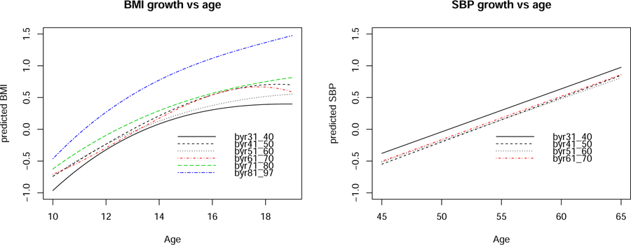
Predicted growth in adolescent BMI and middle-age SBP controlling for onset and historical time of a visit.

Figure 3 exhibits the normal probability plots of the level-2 and −1 residuals from the joint model that produced the estimates in Table 3. Modest heavy tails are noticeable in some level-2 plots, in particular, for those of the random intercepts. This may be because as many as 296 adolescents and 139 adults have only zero to 2 repeated measurements observed in BMI and SBP, respectively, essentially downsizing effective sample sizes for the model fit. This may also be because of omitted covariates we were unable to control such as socioeconomic and environmental covariates unavailable in FLS. A nonnormal model more flexible with heavy tails might have resulted in an improved fit. Other than the moderate heavy tails, the residuals do not appear to deviate severely from the assumed model.

Figure 3:

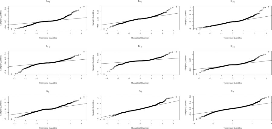
Residual plots of the joint model that produced estimates in Table 3.

We repeated the analysis with an extra covariate, indicating if an individual was taking medication at the time of measurement, added to B_Rij and B_Ctj of the joint model. The total number of visits on medication happened at 22 adolescent and 53 middle-age occasions. Neither the significant effect of the covariate was found on either BMI or SBP, nor did the added covariate change the estimates in Table 3 in a notable way.

6. Discussion

We analyzed the repeated measurements of adolescent BMI and middle-age SBP nested within 835 female participants of FLS to estimate the lasting effects of growth rates in BMI and menarche, including the growth rates-by-age and menarche-by-age interaction effects, on SBP later in middle age via a multilevel GCM, controlling for onset of cancer, age, birth year cohort, and historical time of measurement. Estimation of the GCM was nonstandard and computationally intensive because BMI and SBP were repeatedly measured on two distinct sets of unbalanced time points nested within each participant, and missing values were substantial on BMI, SBP and menarche.

For efficient estimation by all observed data, we estimated the multilevel joint distribution of SBP, BMI and menarche assumed MAR given known covariates by ML via the EM algorithm. A series of likelihood ratio tests revealed that the coefficients of the linear, quadratic and cubic age terms on BMI and linear age on SBP vary randomly across individuals and that cohort effects are significant on menarche and random coefficients except the random slope of age on SBP. We transformed the estimated joint model to the desired GCM by the delta method. Because we analyzed FLS female participants who are mostly white, our findings are most appropriately applicable to European Americans. We illustrated unbiased estimation by our method via simulation.

The estimated mean growth trajectory in adolescent BMI is much higher among individuals born in 1981 to 1997 than those in earlier cohorts such that the mean differences are most striking, ranging 0.66 to 1.08 SDs on average, by age 19 as shown in Figure 2. Because middle-age measurements of those born in 1981 or later are not yet available, we are unable to show the impact on middle-age SBP. When they become available, we anticipate that the impact will strengthen quite remarkably.

We found only modest effect sizes of growth rates in adolescent BMI and menarche on SBP in our analysis. That may be because we have ignored an important family level. Because 376 family members and relatives who accompanied 459 participants enrolled at birth to clinics for measurement were also measured, analysis of the repeated measurements of individuals nested within families would have resulted in more efficient estimates, which will be an important future analysis.

Because FLS started collecting socioeconomic covariates such as income and education quite recently since the year 2002, we could not control for the effects of such covariates. The omitted covariates may have contributed to the modest effect sizes we found. A valuable future research is to reanalyze the GCM, combining FLS with other longitudinal samples that have collected extensive socioeconomic covariates. Our missing data method can be extended to handle such analysis of multiple samples.

The FLS female sample comprises 1,196 occasions of 436 subjects to give 2.7 occasions per middle-age female. In addition, missing data are substantial on BMI, SBP and menarche. Consequently, the FLS female sample sizes may not have provided adequate power to detect the desired effects. Furthermore, adolescence and middle age may be too distant to reveal significant associations between BMI and SBP, possibly, due to confounders. In near future, we want to reanalyze the model in a way that increases sample sizes and also in a way that involves closer timeframes. For example, we may estimate the effects of growth rates in teenagers’ obesity on an earlier adulthood outcome by the entire sample.

Adolescent obesity may also be too distant in time to reveal direct effects on middle-age health. What we have found in this paper may be the evidence of a lack of the direct effects of growth rates in adolescent obesity on middle-age health, and important mediators may exist in closer future. For example, it is plausible that the effects of adolescent obesity on middle-age health are mediated by a near-future health outcome in earlier adulthood. Although we have illustrated the impact of a univariate BMI in adolescence on a univariate SBP in middle age, extension to multivariate health outcomes is straightforward.

Under our current model, we assumed constant variances σ_RR and σ_CC of occasion-specific or within-person random errors of middle-age SBP and adolescent BMI, respectively. In near future, we want to estimate non-constant error variances σ_RRj and σ_CCj of person j such that the person-specific random coefficients of SBP are correlated with the within-person variances log(σ_RRj) and log(σ_CCj) (Hedeker et al. 2008). We will also consider the non-constant variances of the SBP and BMI growth trajectories, for example, across males and females in an extended FLS analysis.

References

- Bock RD and Lieberman M (1970). Fitting a Response Model for n Dichotomously Scored Items. Psychometrika, 35, 179–197. [Google Scholar]
- Bauer DJ (2003). Estimating Multilevel Linear Models as Structural Equation Models, Journal of Educational and Behavioral Statistics, 28, 135–167. [Google Scholar]
- Bollen KA (1989). Structural equations with latent variables. New York: John Wiley & Sons. [Google Scholar]
- Bollen KA and Curran PJ (2006). Latent curve models: A structural equation perspective, Hoboken, NJ: Wiley [Google Scholar]
- Caspi A, Houts RM, Belsky DW, Harrington H, Hogan S, Ramrakha S, Poulton R and Moffitt TE (2016). Childhood forecasting of a small segment of the population with large economic burden, Nature Human Behavior, 1, 1–10. [DOI] [PMC free article] [PubMed] [Google Scholar]
- Casella G and Berger RL (2002). Statistical Inference, Belmont, CA: Duxbury [Google Scholar]
- Dempster AP, Laird NM, and Rubin DB (1977). Maximum Likelihood From Incomplete Data via the EM Algorithm. Journal of the Royal Statistical Society: Series B, 76, 1–38. [Google Scholar]
- Dempster AP, Rubin DB and Tsutakawa RK (1981). Estimation in Covariance Components Models. Journal of the American Statistical Association, 76, 341–353. [Google Scholar]
- Eriksson JG, Forsen T, Tuomilehto J, Winter PD, Osmond C and Barker DJ (1999). Catch-up growth in childhood and death from coronary heart disease: longitudinal study. BMJ, 318, 427–431. [DOI] [PMC free article] [PubMed] [Google Scholar]
- Felitti VJ, Anda RF, Nordenberg D, Williamson DF, Spitz AM, Edwards V, Koss MP and Marks JS (1998). Relationship of childhood abuse and household dysfunction to many of the leading causes of death in adults. The Adverse Childhood Experiences (ACE) Study. American Journal of Preventive Medicine, 14, 245–258. [DOI] [PubMed] [Google Scholar]
- Ferreira I, Twisk JW, van Mechelen W, Kemper HC,Stehouwer CD (2005) Development of fatness, fitness, and lifestylefrom adolescence to the age of 36 years: determinants of the metabolic syndrome in young adults. The Amsterdam growth and health longitudinal study. Arch. Intern. Med, 165, 42–48. [DOI] [PubMed] [Google Scholar]
- Goldstein H and Browne W (2002). Multilevel factor analysis modeling using Markov Chain Monte Carlo estimation In Marcoulides G and Moustaki I eds. Quantitative methodology series. Latent variable and latent structure models, Mahwah, NJ, US: Lawrence Erlbaum Associates Publishers, 225–243. [Google Scholar]
- Goldstein H (2003). Multilevel Statistical Models, London: Edward Arnold. [Google Scholar]
- Goldstein H, Carpenter J, Kenward MG and Levin KA (2009). Multilevel models with multivariate mixed response types, Statistical Modeling, 9, 173–197. [Google Scholar]
- Goldstein H and Kounali D (2009). Multilevel multivariate modeling of childhood growth, numbers of growth measurements and adult characteristics, Journal of the Royal Statistical Society: Series A, 172, 599–613. [Google Scholar]
- Grilli L and Rampichini C (2011). The role of sample cluster means in multilevel models: A view on endogeneity and measurement error issues. Methodology: European Journal of Research Methods for the Behavioral and Social Sciences, 7, 121–133. [Google Scholar]
- Grimm KJ and Ram N (2009). Nonlinear Growth Models in Mplus and SAS. Structural Equation Modeling, 16, 676–701. [DOI] [PMC free article] [PubMed] [Google Scholar]
- Gueorguieva R (2001). A multivariate generalized linear mixed model for joint modeling of clustered outcomes in the exponential family, Statistical Modeling, 1, 177–193. [Google Scholar]
- Hedeker D and Gibbons RD (1994). Application of Random-Effects Pattern-Mixture Models for Missing Data in Longitudinal Studies, Psychological Methods, 2, 64–78. [Google Scholar]
- Hedeker D, Mermelstein RJ and Demirtas H (2008). An Application of a Mixed-Effects Location Scale Model for Analysis of Ecological Momentary Assessment (EMA) Data. Biometrics, 64(2), 627–634. [DOI] [PMC free article] [PubMed] [Google Scholar]
- Ivanova A, Molenberghs G and Verbeke G (2016). Mixed models approaches for joint modeling of different types of responses, Journal of Biopharmaceutical Statistics, 26, 601–618. [DOI] [PubMed] [Google Scholar]
- Kim N, Sabo RT, Wang A, Sabo CS and Sun SS (2016). Effects of Curtailed Juvenile State on Cardiac Structure and Function in Adulthood: The Fels Longitudinal Study, Journal of Child Obesity, 1, 1–8. [DOI] [PMC free article] [PubMed] [Google Scholar]
- Law CM, Shiell AW, Newsome CA, Syddall HE, Shinebourne EA, Fayers PM, Martyn CN and de Swiet M (2002). Fetal, Infant, and Childhood Growth and Adult Blood Pressure. Circulation, 105, 1088–1092. [DOI] [PubMed] [Google Scholar]
- Liu M, Taylor JMG, and Belin TR (2000). Multiple Imputation and Posterior Simulation for Multivariate Missing Data in Longitudinal Studies. Biometrics, 56 1157–63. [DOI] [PubMed] [Google Scholar]
- Lüdtke O, Marsh HW, Robitzsch A, Trautwein U, Asparouhov T, and Muthén B (2008). The Multilevel Latent Covariate Model: A New, More Reliable Approach to Group-Level Effects in Contextual Studies, Psychological Methods, 13, 203–229. [DOI] [PubMed] [Google Scholar]
- MacCallum RC, Kim C, Malarkey W and Kielcolt-Glaser J (1997). Studying multivariate change using multilevel models and latent curve models. Multivariate Behavioral Research, 32, 215–253. [DOI] [PubMed] [Google Scholar]
- McLeod GF, Fergusson DM, Horwood LJ, Boden JM and Carter FA (2018). Childhood predictors of adult adipose: findings from a longitudinal study, The New Zealand Medical Journal, 131(1472), 10–20. [PubMed] [Google Scholar]
- Moffitt TE, Arsenate L, Bel sky D, Dickson N, Han cox RJ, Harrington H, et al. (2011). A gradient of childhood self-control predicts health, wealth, and public safety. Proceedings of the National Academy of Sciences USA, 108, 2693–98. [DOI] [PMC free article] [PubMed] [Google Scholar]
- Nooyens ACJ, Koppes LLJ, Visscher TLS, Twisk JWR, Kemper HCG, Schuit AJ, van Mechelen W, Seidell JC (2007). Adolescent skinfold thickness is a better predictor of high body fatness in adults than is body mass index: the Amsterdam Growth and Health Longitudinal Study, The American Journal of Clinical Nutrition, 85, 1533–9. [DOI] [PubMed] [Google Scholar]
- Olsen MK and Schafer JL (2001). A Two-Part Random-Effects Model for Semi continuous Longitudinal Data, Journal of the American Statistical Association, 96, 730–745. [Google Scholar]
- Preacher KJ, Switchman AL, Malacca RC and Briggs NE (2008). Latent Growth Curve Modeling. Sage: Thousand Oaks, CA. [Google Scholar]
- R Core Team (2017). R: A language and environment for statistical computing. R Foundation for Statistical Computing, Vienna, Austria: URL https://www.R-project.org/. [Google Scholar]
- Raghunathan T, Lepkowski J, Van Hoewyk J and Solenberger P (2001). A Multivariate Technique for Multiply Imputing Missing Values Using a Sequence of Regression Models. Survey Methodology, 27, 85–95. [Google Scholar]
- Ram N and Grimm KJ (2015). Growth Curve Modeling and Longitudinal Factor Analysis In Lerner RM (Ed.), Handbook of child psychology and developmental science (pp. 1–31). Hoboken, NJ: John Wiley & Sons, Inc. [Google Scholar]
- Raudenbush SW, Yang M, Yosef M (2000). Maximum Likelihood for Generalized Linear Models with Nested Random Effects via High-Order, Multivariate Laplace Approximation. Journal of Computational and Graphical Statistics, 9, 141–157. [Google Scholar]
- Raudenbush SW and Bryk AS (2002). Hierarchical Linear Models. Newbury Park, CA: Sage. [Google Scholar]
- Ren C and Shin Y (2016) Longitudinal Latent Variable Models Given Incompletely Observed Biomarkers and Covariates, Statistics in Medicine, 35, 4729–45. [DOI] [PMC free article] [PubMed] [Google Scholar]
- Roberts BW, Kuncel NR, Shiner R, Caspi A and Goldberg LR (2007). The power of personality: the comparative validity of personality traits, socioeconomic status, and cognitive ability for predicting important life outcomes. Perspectives on Psychological Science, 2, 313–345. [DOI] [PMC free article] [PubMed] [Google Scholar]
- Roche A (1992). Growth, maturation and body composition: the Fels longitudinal study 1929–1991. United Kingdom: Cambridge University Press. [Google Scholar]
- Rubin DB (1976). Inference and missing data. Biometrika, 63, 581–592. [Google Scholar]
- Sabo RT, Lu Z, Daniels S and Sun SS (2012). Serial Childhood BMI and associations With Adult Hypertension and Obesity: the Fels Longitudinal study, Obesity, 20, 1741–43. [DOI] [PMC free article] [PubMed] [Google Scholar]
- Sabo RT, Yen M, Daniels S and Sun SS (2014). Associations between Childhood Body Size, Composition, Blood Pressure and Adult Cardiac Structure: The Fels Longitudinal Study, PLoS ONE, 9, 1–10. [DOI] [PMC free article] [PubMed] [Google Scholar]
- Sabo RT, Wang A, Deng Y, Sabo CS and Sun SS (2017). Relationships between childhood growth parameters and adult blood pressure: the Fels Longitudinal Study, Journal of Developmental Origins of Health and Disease, 8, 113–122. [DOI] [PubMed] [Google Scholar]
- Schafer JL and Yucel RM (2002). Computational Strategies for Multivariate Linear Mixed-Effects Models with Missing Values. Journal of Computational and Graphical Statistics, 11, 437–457. [Google Scholar]
- Shin Y and Raudenbush SW (2007). Just-Identified Versus Over-Identified Two-Level Hierarchical Linear Models with Missing Data. Biometrics, 63, 1262–68. [DOI] [PubMed] [Google Scholar]
- Shin Y and Raudenbush SW (2010). A Latent Cluster Mean Approach to The Contextual Effects Model with Missing Data. Journal of Educational and Behavioral Statistics, 35, 26–53. [Google Scholar]
- Shin Y and Raudenbush SW (2020). Income Equality in Achievement among US Elementary Schools: A Random Coefficients Model with Data MAR. Manuscript in preparation.
- Stram DO and Lee J (1994). Variance Components Testing in the Longitudinal Mixed Effects Model. Biometrics, 50, 1171–77. [PubMed] [Google Scholar]
- Sun SS, Grave GD, Siervogel RM, Pickoff A, Arslanian S, and Daniels SR (2007). Systolic Blood Pressure in Childhood Predicts Hypertension and the Metabolic Syndrome Later in Life. Pediatrics, 119, 237–46. [DOI] [PubMed] [Google Scholar]
- Sun SS, Liang R, Huang TT, Daniels SR, Arslanian S, Liu K, Grave GD, and Siervogel RM (2008). Childhood obesity predicts adult metabolic syndrome: the Fels Longitudinal Study. The Journal of Pediatrics, 152, 191–200. [DOI] [PMC free article] [PubMed] [Google Scholar]
- van Buuren S, Brand J, Groothuis-Oudshoorn C, and Rubin D (2006). Fully conditional specification in multivariate imputation. Journal of Statistical Computation and Simulation, 76, 1049–64 [Google Scholar]
- van Buuren S (2011). Multiple imputation of multilevel data In Hox JJ and Roberts JK (Eds.), The Handbook of Advanced Multilevel Analysis, Chapter 10, pp. 173–196. Milton Park, UK: Routledge. [Google Scholar]
- Wang M and Bodner T (2007). Growth Mixture Modeling: Identifying and Predicting Unobserved Subpopulations with Longitudinal Data. Organizational Research Methods, 10, 635–656. [Google Scholar]
- Willett JB and Sayer AG (1994). Using covariance structure analysis to detect correlates and predictors of individual change over time. Psychological Bulletin, 116, 363–381. [Google Scholar]