A Hierarchical Bayesian Model for Differential Connectivity in Multi-trial Brain Signals

Abstract

There is a strong interest in the neuroscience community to measure brain connectivity and develop methods that can differentiate connectivity across patient groups and across different experimental stimuli. The development of such statistical tools is critical to understand the dynamics of functional relationships among brain structures supporting memory encoding and retrieval. However, the challenge comes from the need to incorporate within-condition similarity with between-conditions heterogeneity in modeling connectivity, as well as how to provide a natural way to conduct trial- and condition-level inference on effective connectivity. A Bayesian hierarchical vector autoregressive (BH-VAR) model is proposed to characterize brain connectivity and infer differences in connectivity across conditions. Within-condition connectivity similarity and between-conditions connectivity heterogeneity are accounted for by the priors on trial-specific models. In addition to the fully Bayesian framework, an alternative two-stage computation approach is also proposed which still allows straightforward uncertainty quantification of between-trial conditions via MCMC posterior sampling, but provides a fast approximate procedure for the estimation of trial-specific VAR parameters. A novel aspect of the approach is the use of a frequency-specific measure, partial directed coherence (PDC), to characterize effective connectivity under the Bayesian framework. More specifically, PDC allows inferring directionality and explaining the extent to which the present oscillatory activity at a certain frequency in a sender channel influences the future oscillatory activity in a specific receiver channel relative to all possible receivers in the brain network. The proposed model is applied to a large electrophysiological dataset collected as rats performed a complex sequence memory task. This unique dataset includes local field potentials (LFPs) activity recorded from an array of electrodes across hippocampal region CA1 while animals were presented with multiple trials from two main conditions. The proposed modeling approach provided novel insights into hippocampal connectivity during memory performance. Specifically, it separated CA1 into two functional units, a lateral and a medial segment, each showing stronger functional connectivity to itself than to the other. This approach also revealed that information primarily flowed in a lateral-to-medial direction across trials (within-condition), and suggested this effect was stronger on one trial condition than the other (between-conditions effect). Collectively, these results indicate that the proposed model is a promising approach to quantify the variation of functional connectivity, both within- and between-conditions, and thus should have broad applications in neuroscience research.

1. Introduction

Brain electrophysiological signals, including local field potentials (LFPs) and electroencephalograms (EEGs), offer important insight into the neural mechanisms underlying learning and memory, as they capture the electrical activity of groups of neurons at a temporal resolution of milliseconds. Compared to scalp EEG, LFP recordings are typically performed in animal experiments using electrodes chronically implanted inside the brain. Consequently, LFPs recordings allow us to directly probe neural activity deep in the brain with little contamination from non-neuronal physiological activity (e.g., artifacts from muscle activity). While LFP recordings have been performed in many brain regions, the hippocampus has been a primary focus of electrophysiological studies because of its well-established role in memory (O’Keefe [1993]; Buzsáki [1996]; McNaughton et al. [2006]; Eichenbaum et al. [2007]; Squire and Wixted [2011]). Accumulating evidence suggests that the hippocampus plays a key role in remembering the sequence of daily life events. In order to elucidate the neuronal mechanisms underlying the capacity, Dr. Fortin’s laboratory on memory and learning recently developed a complex non-spatial sequence memory task in rats (Allen et al. [2014]). Importantly, the task has been shown to have strong behavioral parallels in rats and humans (Allen et al. [2014]), and to depend on comparable brain circuits across species (Fortin et al. [2016]; Boucquey et al. [2015, submitted]).

Here, we focus on an electrophysiological dataset collected as rats performed this new behavioral task, in which they used an array of electrodes distributed within hippocampal region CA1 (Allen et al. [2016]; see Figure 13). Of particular interest is the fact that their experimental approach allows us to compare LFP activity between two main trial conditions: one in which stimuli were presented in the correct sequence (i.e., “in sequence” or InSeq; e.g., ABC…), and another in which one of the stimuli was presented in an incorrect sequence position (i.e., “out of sequence” or OutSeq; e.g., ABD…). Figure 1 shows example LFP traces recorded in one trial/epoch (here an epoch is 1 second time block) from the two trial conditions (InSeq and OutSeq). Very different temporal patterns of LFPs can be observed between the two trial conditions, suggesting potential variations in hippocampal LFP activity across trials and/or conditions. Therefore, this dataset offers a unique opportunity to investigate functional connectivity in the hippocampus, particularly its potential variation across trials (within-condition) and differentiation across trial conditions (between-conditions; i.e., InSeq vs OutSeq).

Figure 1:

Local field potential (LFP) recordings from 12 tetrodes during one trial (1000 milliseconds; T = 1000) under InSeq and OutSeq condition respectively. Each time series indicates the LFP recording from one tetrode. Different temporal patterns could be indication of different effective connectivities between tetrodes. These LFPs have temporal patterns that can be separated into two main groups: a lateral CA1 group (T2, T9, T8, and T7) and a medial CA1 group (T14, T23, T16, T22, T19 and T20). For clarity, the electrodes near the transition point (T15 and T13) are not included in either group. Note the difference in LFP waveforms between the two trial conditions (e.g., lower beta power on OutSeq trial than InSeq trial).

To analyze multi-trial LFPs at the condition level, Hu et al. [2017] have proposed a two-stage modeling approach where vector auto-regressive (VAR) models are employed to characterize each individual trial separately and estimate trial-specific connectivities in the first stage, then estimate the between-conditions variation of the estimated connectivities in the second stage. However, their approach has some drawbacks. First, the parameter estimation procedure does not take into account the similarity of connectivity structure within the same condition, since trials from the same experimental condition are modeled and estimated separately. Second, summarizing and making inference on the condition-level effective connectivity is accomplished via bootstrap analysis, where the random variability at the trial level is introduced but not accounted for by re-sampling the residuals. In this paper, we address those deficiencies by employing a Bayesian hierarchical vector autoregressive (BH-VAR) framework (Chiang et al. [2017]). By imposing condition-level priors on the parameters in trial-specific models, the proposed hierarchical modeling approach allows to take simultaneously into account both within-condition correlation and between-conditions variation. The prior information will help to improve the characterization of trial-specific and condition-level connectivity through the posterior distribution. Further, our proposed approach takes into account potential sparse structure in high dimensional parameter space of brain signals by inducing sparsity in parameters via “spike-and-slab” mixture priors.

To describe condition-specific effective connectivities, we propose the use of partial directed coherence (PDC) (Baccalá and Sameshima [2001] and Baccalá and Sameshima [2014]). PDC is a measure of connectivity in the frequency domain. Compared to the connectivity simply characterized by coefficients of VAR matrices, PDC gives a deeper characterization of how an oscillatory activity (at a particular frequency band) at a present time in one tetrode may impact oscillatory activity of the same frequency band at another tetrode at a future time point. With respect to other measures of connectivity typically used in the frequency domain (e.g., coherence, partial coherence) (Ombao and Van Bellegem [2006]; Fiecas et al. [2011]; Olhede and Ombao [2013]; Gorrostieta et al. [2019]), PDC is thus able to imply the direction of information flow between tetrodes, an information that investigators may find particularly useful. The remainder of this paper is arranged as follows. In Section 2, we present the details of proposed hierarchical Bayesian models followed by simulation studies in Section 3. Analysis of LFP signals is in Section 4 and the Conclusion is in Section 5.

2. A Bayesian hierarchical VAR model for differential connectivity

2.1. Single stage modeling

A P-dimensional LFP signal from trial s under condition g is said to follow a Bayesian hierarchical VAR model of order d, denoted as BH-VAR(d), if it can be expressed as

$$\left(X_{t,g}^{(s)}\mid {\eta }_s=g,{\Phi }_{\mathcal{l},g}^{(s)},\Sigma \right)=\sum _{\mathcal{l}=1}^d{\Phi }_{\mathcal{l},g}^{(s)}{X}_{t-\mathcal{l},g}^{(s)}+{\epsilon }_t^{(s)}t=d+1,\mathrm{..},T,$$ (2.1)

where η_s is a condition indicator, s = 1, …, n, and g = 1, …, G. Since hippocampal processes are not identical across trials even during the same condition (Allen et al. [2016]; Ng et al. [2018]), we don’t assume universal deterministic part for VAR models at the condition level. The matrices ${\Phi }_{\mathcal{l},g}^{(s),}\text{s}\in {\Re }^{P\times P}$ are the autoregressive coefficient matrices of trial s from condition g, which capture lagged cross-dependence among signals from different tetrodes in trial s. We assume ${\epsilon }_t^{(s)}\stackrel{iid}{~}N(\underset{\_}{0},\Sigma )$ for the noise of trial s. For the sake of simplifying the model and reducing the number of parameters, the VAR covariance matrix Σ is assumed to be a diagonal matrix, diag{σ₁, …, σ_P}, with hyper priors σ_j~ IG(h₁, h₂) (j = 1, …, P) placed on σ_j’s. Priors $p\left({\Phi }_{\mathcal{l},g}^{(s)}\mid {\Phi }_{\mathcal{l},g}\right)(\mathcal{l}=1,\dots ,d)$ are imposed to account for the between-trials variation on VAR matrices under condition g, where ${\left\{{\Phi }_{\mathcal{l},g}\right\}}_{\mathcal{l}=1}^d$ indicate the condition-specific coefficient matrices. An illustration of condition-specific connectivity via the BH-VAR model can be found in Figure 2. Denote the LFP recording of neurons to be u-th and v-th tetrode. Then the entry ${\Phi }_{\mathcal{l},g}^{uv}(g=1,2)$ shows the impact of the input from v-th tetrode at time $t-\mathcal{l}$ to brain activity at u-th tetrode at the current time t under condition g. If ${\Phi }_{\mathcal{l},g}^{uv}=0$ and ${\Phi }_{\mathcal{l},g}^{vu}=0$ for all lags $\mathcal{l}$ then, there is no directed connectivity from node u to node v as determined by the BH-VAR model under condition g. Thus, the entries of ${\left\{{\Phi }_{\mathcal{l},g}\right\}}_{\mathcal{l}=1}^d$ contain all the information about brain connectivity between tetrodes under condition g.

Figure 2:

LFP traces and VAR. ${\Phi }_{\mathcal{l},g}^{uv}(\mathcal{l}=1,2)$ captures the impact of the input from v-th tetrode at time $t-\mathcal{l}$ to brain activity at u-th tetrode at the current time t from condition g.

Note that model (2.1) can be written in a standard multivariate linear regression form

$$\underset{Y_g^{(s)};(T-d)\times P}{\underbrace{\left[\begin{array}{c}{\left(X_{T,g}^{(s)}\right)}^{\prime }\\ ⋮\\ {\left(X_{d+1,g}^{(s)}\right)}^{\prime }\end{array}\right]}}=\underset{{\mathbb{X}}_g^{(s)}:(T-d)\times Pd}{\underbrace{\left[\begin{array}{ccc}{\left(X_{T-1,g}^{(s)}\right)}^{\prime }& \cdots & {\left(X_{T-d,g}^{(s)}\right)}^{\prime }\\ ⋮& \ddots & ⋮\\ {\left(X_{d,g}^{(s)}\right)}^{\prime }& \cdots & {\left(X_{1,g}^{(s)}\right)}^{\prime }\end{array}\right]}}\underset{B_g^{(s)}:Pd\times P}{\underbrace{\left[\begin{array}{c}{\left({\Phi }_{1,g}^{(s)}\right)}^{\prime }\\ ⋮\\ {\left({\Phi }_{d,g}^{(s)}\right)}^{\prime }\end{array}\right]}}+\underset{E^{(s)}:(T-d)\times P}{\underbrace{\left[\begin{array}{c}{\left({\epsilon }_T^{(s)}\right)}^{\prime }\\ ⋮\\ {\left({\epsilon }_{d+1}^{(s)}\right)}^{\prime }\end{array}\right]}}.$$ (2.2)

Use the vec notation

$$y_g^{(s)}=vec\left(Y_g^{(s)}\right)$$

$${\beta }_g^{(s)}=vec\left(B_g^{(s)}\right)$$

$$e^{(s)}=vec\left(E^{(s)}\right)$$

where vec(Y_g^(s)) stacks the columns of Y_g^(s) on tops of one another. Then we must have

$$\underset{(T-d)P\times 1}{\underbrace{y_g^{(s)}}}=(\underset{P\times P}{\underbrace{I}}\otimes \underset{(T-d)\times Pd}{\underbrace{{\mathbb{X}}_g^{(s)}}})\underset{P^{2}d\times 1}{\underbrace{{\beta }_g^{(s)}}}+\underset{(T-d)P\times 1}{\underbrace{e^{(s)}}},$$ (2.3)

where $e^{(s)}~N(\underset{\_}{0},\Sigma \otimes I)$. Eventually we can write model (2.1) as

$$\left(y_g^{(s)}\mid {\beta }_g^{(s)},\Sigma \right)~N\left(\left(I\otimes {\mathbb{X}}_g^{(s)}\right){\beta }_g^{(s)},\Sigma \otimes I\right),$$ (2.4)

with ${\beta }_g^{(s)}$ capturing the trial-level connectivities.

Here we adopt the model in Chiang et al. [2017] and Gorrostieta et al. [2013], and propose to model the condition-level connectivities φ_g (vectorized VAR matrices at condition g). Multivariate normal priors are put on ${\beta }_g^{(s)}$:

$$\left({\beta }_g^{(s)}\mid {\phi }_g,{\Xi }_g\right)~N\left({\phi }_g,{\Xi }_g\right).$$ (2.5)

The trial-level connectivities under condition g are modeled as random deviations from the baseline process of condition g, where ${\Xi }_g=\text{diag}\left\{{\xi }_{g,1},\dots ,{\xi }_{g,d{P}^2}\right\}$ is a diagonal covariance matrix to account for the variation.

In particular, we enforce sparsity in the condition-level connectivity structure by imposing “spike-and-slab” mixture priors (Mitchell and Beauchamp [1988]; George and McCulloch [1993]; George and McCulloch [1997]) on elements of φ_g. By weeding out less important parameters, the proposed approach aims to improve accuracy of estimated effective connectivity. Denote elements of φ_g by ${\left\{{\phi }_{g,k}\right\}}_{k=1,\dots ,d{P}^2}$, we introduce binary indicators ${\left\{{\gamma }_{g,k}\right\}}_{k=1,\dots ,d{P}^2}$, which satisfy γ_g,k = 1 if φ_g,k is non-zero and γ_g,k = 0 otherwise. Then our “spike-and-slab” priors are defined as follows

$$\left({\phi }_{g,k}\mid {\gamma }_{g,k}\right)~{\gamma }_{g,k}N\left(0,{\tau }_0^2\right)+\left(1-{\gamma }_{g,k}\right){\delta }_0\left({\phi }_{g,k}\right),$$ (2.6)

where δ₀(φ_g,k) is a point mass density at φ_g,k = 0, and ${\tau }_0^2$ is constant. Typically, ${\tau }_0^2$ is chosen large enough to allow estimating large deviations from the null hypothesis. Taking into account the potential difference in variation of zero and non-zero elements of trial-level parameters ${\beta }_g^{(s)}$ in Equation (2.5), we also put priors on the diagonal elements of Ξ_g to differentiate the variances conditional on zero and non-zero elements of φ_g. If γ_g,k = 1, we set ${\xi }_{g,k}=c_g^1~IG\left(a_g^1,b_g^1\right)$; if γ_g,k = 0, ${\xi }_{g,k}=c_g^0~IG\left(a_g^0,b_g^0\right)$, where $\left(a_g^1,b_g^1,a_g^0,b_g^0\right)$ are constants. Furthermore, we impose Bernoulli priors on the variable selection indicator γ_g,k

$$\left({\gamma }_{g,k}\mid p_g\right)~\mathit{\text{Bern}}\left(p_g\right),k=1,\dots ,d{P}^2.$$ (2.7)

p_g is the probability of non-zero VAR parameters at condition-level and follows $p_g~\mathit{\text{Beta}}\left({\alpha }_g^1,{\alpha }_g^2\right)$. The value of $\left({\alpha }_g^1,{\alpha }_g^2\right)$ is informed via prior information on the proportion of non-zero dependence of LFPs. The graphical structure of our proposed BH-VAR model can be found in Figure 3. Nodes in circles denote parameters, while nodes in squares denote observables based on LFPs.

Figure 3:

Graphical structure of the proposed probabilistic model in BH-VAR. Nodes in circles denote parameters, and nodes in squares denote observables based on LFPs.

2.2. Fast two-stage computation in a quasi-Bayesian approach

Since the computation of the above fully Bayesian approach is very intensive, one contribution of this manuscript is an alternative two-stage computation approach which still allows straightforward uncertainty quantification of between-trial conditions via a Bayesian hierarchical model and MCMC posterior sampling, but provides a fast approximate procedure for the estimation of trial-specific VAR parameters. In the first stage, we use least squares estimation (LSE) to obtain estimated trial-specific VAR parameters $\widehat{{\beta }_g^{(s)}}$, which satisfy

$$\widehat{{\beta }_g^{(s)}}=\underset{{\beta }_g^{(s)}\in {\Re }^{P^{2}d}}{\text{argmin}}{\Vert y_g^{(s)}-\left(I\otimes {\mathbb{X}}_g^{(s)}\right){\beta }_g^{(s)}\Vert }^2.$$ (2.8)

In the second stage, we consider the parameters estimated in the first stage, and apply Step 2–6 of the above algorithm at each MCMC iteration to draw posterior samples of the condition-level VAR parameters φ_g and their corresponding binary indicators γ_g.

The proposed approach avoids sampling ${\beta }_g^{(s)}$ from high dimensional multivariate normal distribution (for example, dimension is P² × d × n in this case) and computing their high dimensional covariance matrix. As a result, it can save the computation of P² × d × n parameters at each iteration. The computational improvement comes at the cost of potentially underestimating the uncertainty of trial-specific parameters in Step 1. Here, one the one hand, we are primarily interested in identifying the non-zero connectivities by leveraging the information between trials and within group, and on the other hand we will show that the estimation results of condition-level parameters are almost not affected in a simulation study in Section 3.

2.3. Inference on condition-level non-zero VAR parameters

In the Bayesian VAR model (2.1), we conclude there exists no connectivity from tetrode v to tetrode u during condition g at lag $\mathcal{l}$ if ${\Phi }_{\mathcal{l},g}^{uv}=0$, which is equivalent to γ_g,k = 0, where γ_g,k is the corresponding binary indicator in “spike-and-slab” priors (2.6). Basically this requires dP² null hypotheses $H_0^k:{\gamma }_{g,k}=0$ to be tested, which leads to a multiple hypotheses testing problem. To conduct inference on this, we adopt a Bayesian decision theoretic perspective, and compute marginal posterior probabilities (MPP) of $p\left({\gamma }_{g,k}=1\mid y_g^{(s)},s=1,\dots ,n\right)$. The MPP’s are estimated as the proportions of MCMC samples such that γ_g,k = 1 across all iterations after burn-in. A threshold on the MPP’s leads to an optimal decision rule under a loss function which is a weighted compounded linear function of false positives and false negatives. We further choose the threshold κ_g to control the Bayesian false discovery rate (BFDR) at a certain level 0.05, that is

$$\text{BFDR}\left({\kappa }_g\right)=\frac{{\sum }_{k=1}^{d{P}^2}\left(1-{\text{MPP}}_k^{(g)}\right)I_{\left({\text{MPP}}_k^{(g)}>{\kappa }_g\right)}}{{\sum }_{k=1}^{d{P}^2}{I}_{\left({\text{MPP}}_k^{(g)}>{\kappa }_g\right)}}.$$ (2.9)

${\kappa }_g^{*}$ and ${\kappa }_g^{**}\left({\kappa }_g^{*}<{\kappa }_g<{\kappa }_g^{**}\right)$ are selected to ensure interval $\left(\text{BFDR}\left({\kappa }_g^{**}\right),\text{BFDR}\left({\kappa }_g^{*}\right)\right)$ contains BFDR(κ_g) = 0:05. $H_0^k:{\gamma }_{g,k}=0$ is rejected if ${\text{MPP}}_k^{(g)}\ge {\kappa }_g$. In other words, we can conclude lag-specific directional connectivity between certain tetrodes at condition level if their corresponding MPP is above the threshold κ_g.

2.4. Measures of effective connectivity

In this section, we will review several frequency domain connectivity measures typically employed in brain imaging when using the VAR model. We start by recalling that a P-tetrode brain signal, denoted $\left\{X_t={\left(X_t^1,\dots ,X_t^P\right)}^{\prime },t=1,2,\dots \right\}$, is said weakly stationary if

1. E(X_t) is constant over all time t, and

2. the auto-covariance function matrix

   $$cov\left(X_t,X_{t+h}\right)=\Gamma (h)=\left(\begin{array}{cccc}{\gamma }_{11}(h)& {\gamma }_{12}(h)& \dots & {\gamma }_{1P}(h)\\ {\gamma }_{21}(h)& {\gamma }_{22}(h)& \dots & {\gamma }_{2P}(h)\\ ⋮& ⋮& \ddots & ⋮\\ {\gamma }_{P1}(h)& {\gamma }_{P2}(h)& \dots & {\gamma }_{PP}(h)\end{array}\right)$$

   does not depend on t, where ${\gamma }_{uv}(h)=cov\left(X_t^u,X_{t+h}^v\right)$ for all pairs of tetrodes u, v = 1; …, P.

If the sequence of auto- and cross-covariance between any pair of tetrodes u and v is absolutely summable, i.e., ${\sum }_{h=-\infty }^{\infty }\left|{\gamma }_{uv}(h)\right|<\infty$, the spectral density matrix at frequency ω is defined as

$$f(\omega )=\sum _{h=-\infty }^{\infty }\Gamma (h)e^{-2\pi i\omega h},-1/2\le \omega \le 1/2.$$ (2.10)

which is a P × P Hermitian non-negative definite matrix whose diagonal elements f_uu(ω) are the auto-spectra of the tetrodes at frequency ω and the off-diagonal elements f_uv(ω) are the cross-spectra of tetrodes u and v at frequency ω.

Coherence between the u-th and v-th tetrodes at frequency ω, is defined as

$${\rho }_{uv}^2(\omega )=\frac{{|f_{uv}(\omega )|}^2}{f_{uu}(\omega )f_{vv}(\omega )},$$ (2.11)

which can be interpreted as how much of ω-oscillatory component in common shared by tetrode u and tetrode v. A large coherence value between tetrodes u and v could be due to direct connectivity between these two tetrodes or could be indirectly due to the intervening effect of other tetrode(s). Partial coherence can be used to measure the strength of connectivity between a pair of tetrodes controlling for the effects of all other tetrodes

Define g(ω) = f⁻¹(ω) and g_pp(ω) are the diagonal elements of g(ω). Let h(ω) be a diagonal matrix whose elements are $g_{pp}^{-1/2}(\omega )$, and C(ω) = −g(ω)h(ω)g(ω). Then, the partial coherence between the u-th and v-th tetrodes is the modulus squared of the (u, v)-th element of C(ω) (Fiecas et al. [2010]; Fiecas et al. [2011])

$${\zeta }_{uv}^2(\omega )={\left|C_{uv}(\omega )\right|}^2.$$ (2.12)

Here we consider partial directed coherence instead (Baccalá and Sameshima [2001]; Baccalá and Sameshima [2014]). For a BH-VAR(d) model given by Equation (2.1), define

$$A_g(\omega )=I-\sum _{\mathcal{l}=1}^d{\Phi }_{\mathcal{l},g}\text{exp}(-i2\pi \omega \mathcal{l}/\Omega )$$ (2.13)

to be the transform of sequence ${\left\{{\Phi }_{\mathcal{l},g}\right\}}_{\mathcal{l}=1}^d$ at frequency ω, where Ω is the sampling frequency. The partial directed coherence from tetrode v to tetrode u at frequency ω under condition g is defined as

$${\pi }_{uv}^2(\omega )=\frac{{\left|A_g^{uv}(\omega )\right|}^2}{{\sum }_{m=1}^P{\left|A_g^{mv}(\omega )\right|}^2},$$ (2.14)

which measures the direct influence from tetrode v to tetrode u conditional on all the outflow from tetrode v. Since the sum of ${\pi }_{uv}^2(\omega )$ is 1 for fixed v, cross-PDC (u ≠ v) gives an indication of the extent to which present frequency-specific oscillatory activity at ω from a sender tetrode v explains future oscillatory activity at ω in a specific receiver tetrode u relative to all tetrodes in the network. In particular, ${\pi }_{vv}^2(\omega )$ (auto-PDC) indicates how much the oscillatory activity at ω of tetrode v can be explained by its own past after adjusting for the other tetrodes.

Figure 4 demonstrate an example of three brain tetrodes connected in a network and the three different measures. tetrode 1 is connected to tetrode 2 with outflow from 1 to 2; tetrode 2 is connected to tetrode 3 with outflow from 2 to 3; tetrode 1 and 3 are not directly connected. Their connectivity measured by coherence, partial coherence and partial directed coherence are shown in Table 1. Coherence between tetrode 1 and 3 at frequency ω is not zero even though they are not directly connected. Partial coherence between tetrode 1 and 3 at frequency ω removes the intervention of tetrode 2, thus ${\zeta }_{31}^2(\omega )={\zeta }_{13}^2(\omega )=0$. Partial directed coherence between tetrodes only measures direct connectivity and is direction sensitive, consequently ${\pi }_{12}^2(\omega )=0$ and ${\pi }_{21}^2(\omega )\ne 0$.

Figure 4:

An example of connectivity characterized by three different measures. In (c.): there is a direction of information flow from tetrode 1 to 2; and from tetrode 2 to 3. In (a.): indirect connectivity between tetrode 1 and tetrode 3 is measured by coherence, while no directionality is specified by partial coherence in (b.).

Table 1:

A comparison of the three connectivity measures in Figure 4.

Tetrodes	Connectivity measures
	Coherence	Partial coherence	Partial directed coherence
1 and 2	${\rho }_{12}^2(\omega )={\rho }_{21}^2(\omega )\ne 0$	${\zeta }_{12}^2(\omega )={\zeta }_{21}^2(\omega )\ne 0$	${\pi }_{12}^2(\omega )=0$
			${\pi }_{21}^2(\omega )\ne 0$
2 and 3	${\rho }_{23}^2(\omega )={\rho }_{32}^2(\omega )\ne 0$	${\zeta }_{23}^2(\omega )={\zeta }_{32}^2(\omega )\ne 0$	${\pi }_{23}^2(\omega )=0$
			${\pi }_{32}^2(\omega )\ne 0$
3 and 1	${\rho }_{31}^2(\omega )={\rho }_{13}^2(\omega )\ne 0$	${\zeta }_{31}^2(\omega )={\zeta }_{13}^2(\omega )=0$	${\pi }_{31}^2(\omega )=0$
			${\pi }_{13}^2(\omega )=0$

2.5. Model selection

In the previous two-stage approach, VAR models with optimal lag order selected by AIC were fitted for each epoch separately (Hu et al. [2017]). Therefore the selected lag orders were not the same across epochs. For this Bayesian approach, we fit model (2.1) with lag order d ∈ {1, 2, 3} to all epochs separately, which lead to different number of parameters. Then we use the posterior mean of MCMC samples after burn-in to calculate BIC for each model based on Equation (2.4). The optimal lag order $\widehat{d}$ is chosen to return the lowest BIC.

3. Simulation study

A simulation study was conducted to investigate: (1) whether BH-VAR method can recover the connectivity information of multi-trial brain signals from different experimental conditions; and (2) whether the two-stage computation approach is able to recover the same connectivity inference as the full Bayesian method. In terms of assessing connectivity recovery, the first criterion is sensitivity - how well the estimated results identify the zero and non-zero structure of VAR matrices, which can be evaluated by the MPP results. The second criterion is specificity - how close the method can estimate the partial directed coherence compared to the truth, which is the comparison between the posterior mean PDCs and true PDCs.

3.1. Simulation setting

In order to assess the performance of the proposed procedure, we generated n = 50 trials of P = 12 tetrodes from G = 2 conditions (25 trials for each) using VAR(1) models. The location of zero and non-zero entries of the two condition-level VAR matrices was determined by a Bern(0.4) prior. Furthermore, we generated values of non-zero entries from Unif(−0.2, 0.3), and random numbers from Unif(0.3, 0.5) were added to the diagonal entries. Figure 5 demonstrates the true VAR matrices from two conditions, where the blank cells indicate true zeros. Then random matrices with eigenvalues between (−0.2, 0.2) were added to the condition-level matrices to construct 50 trial-specific VAR matrices. The prior choice was informed by previous exploratory analyses of a similar datasets according to the two-stage procedure in Hu et al. [2017]. Finally, we added a random noise from N(0, 1) to each trial and 50 trials were simulated with T = 1000 from those VAR(1) matrices. Selected trials from two conditions can be found in Figure 6 and Figure 7, where different temporal patterns are observed between-conditions.

Figure 5:

The condition-level VAR matrices.

Figure 6:

The simulated signals from condition 1.

Figure 7:

The simulated signals from condition 2.

The simulated trials were then estimated by full Bayesian method and two-stage approach separately with: ${\tau }_0^2=5,\left(h_1,h_2\right)=(2,1)$, $\left(a_g^1,b_g^1,a_g^0,b_g^0\right)=(2,1,2,1)$ and $\left({\alpha }_g^1,{\alpha }_g^2\right)=(0.5,0.5)$. A sensitivity analysis on the values of the prior hyperparameter ${\tau }_0^2$ did not show relevant changes in significant results for values larger than 5. 10,000 MCMC iterations were run for both approaches with 5,000 burn-in. Consequently the posterior distributions of condition-level VAR parameters were formed by the 5,000 MCMC samples.

3.2. Inference on sparse connectivity structures

To investigate whether our methods recover the sparse connectivity structure of the simulated data, we examined the inference on the latent indicators γ_g,k (Figure 8). The subindex k indicates the VAR parameter arranged by column. For example, γ_1,20 corresponds to the (8, 2) entry of Φ_1,1. The threshold was then determined by Equation (2.9), and MPP exceeding the threshold implies that γ_g,k should be non-zero (positive) while MPP within the threshold implies γ_g,k is zero (negative). The black dots indicate true positives, red dots indicate false negatives, and blue dots indicate false positives. Based on the results, the full single-stage Bayesian approach successfully recovered most of the true non-zero connectivity, with few false negatives, whose true values were actually very close to 0. It makes sense even though there were a few false positives in the results, because of the randomness that we added to the trial-specific VAR parameters and the white noise in the simulation setting. Compared to the inference of full Bayesian method, the two-stage approach tends to return lower MPP’s values. This trend is possibly due to the loss of information and lack of borrowing of strength in the two-step estimation process versus the full Bayesian method. However, the BFDR thresholding identified a similar sparse connectivity structure than the one recovered by the fully single-stage Bayesian approach.

Figure 8:

MPP’s by full Bayesian method and two-stage approach. The gray dash line indicates the threshold κ_g. MPP exceeding the threshold implies γ_g,k should be non-zero (positive) while MPP within the threshold implies γ_g,k is zero (negative). The black dots indicate true positives, red dots indicate false negatives, and blue dots indicate false positives.

As for the specificity of condition-level connectivities, Figure 9 shows the comparison between the truth and posterior mean estimate of Φ_1,1 and Φ_1,2 given by different methods, where non-zero posterior mean estimate was forced to zero if the corresponding MPP was smaller than the threshold. The results imply that the estimate obtained by the full single stage Bayesian method is very close to the truth, and the two-stage approach provided similar estimation.

Figure 9:

The posterior mean of estimated condition-level VAR matrices.

The posterior standard deviation comparison between two methods can be found in Figure 10, where dark color indicates larger values. The two-stage approach tended to capture less variability of condition level VAR parameters than full Bayesian approach since it used fixed ${\beta }_g^{(s)}$ in MCMC.

Figure 10:

The posterior standard deviation of estimated condition-level VAR matrices.

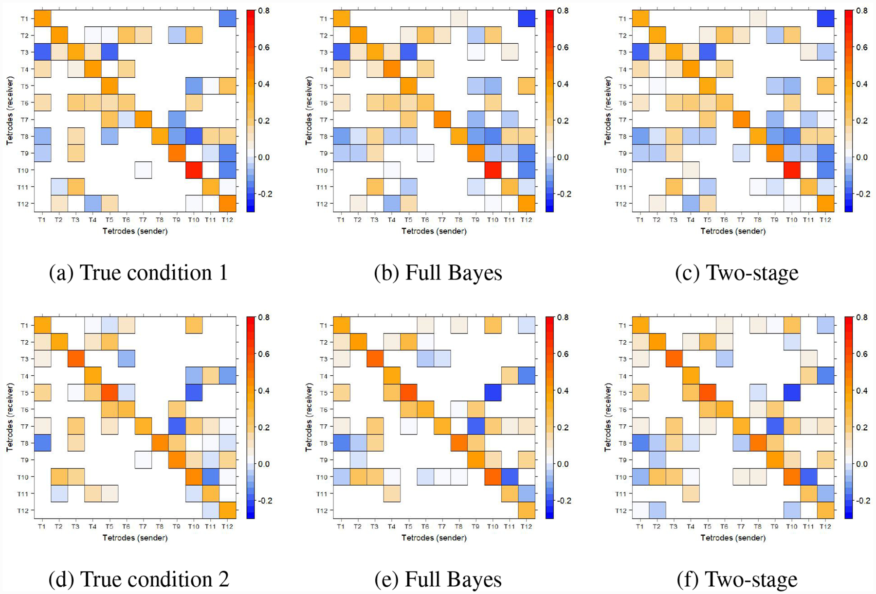
In addition to comparing estimated connectivity via VAR coefficients, comparisons on estimated PDCs were conducted to evaluate the specificity of proposed methods to the connectivity strength at frequency domain. Figure 11 and Figure 12 show the true PDCs and estimated posterior means by two approaches at different condition levels. We can see that both methods recovered the original PDCs.

Figure 11:

The posterior mean of estimated condition-level PDCs at condition 1.

Figure 12:

The posterior mean of estimated condition-level PDCs at condition 2.

4. Application to effective connectivity in multi-trial LFPs

In this section, we fit a BH-VAR model to LFP data recorded from multiple trials under two trial conditions in a non-spatial sequence memory task (InSeq vs OutSeq; Allen et al. [2016]). We aim at estimating the VAR parameters at condition level and the partial directed coherence at several frequency bands of interest. Our objective is to examine and quantify potential connectivity (i,.e., effective) among electrodes located in hippocampal region CA1. This region is clinically meaningful as this form of sequence memory shows strong behavioral parallels in rats and humans (Allen et al. [2014]), and depends on the hippocampus for both species (Fortin et al. [2016], Boucquey et al. [2015, submitted]), and is impaired in normal aging (Allen et al. [2015]).

4.1. Data description

In the experiment (left in Figure 13), rats were presented with repeated sequences of five odors in a single odor port. They were trained to identify whether each odor was presented “in sequence” (by holding their nose poke until the signal delivered after 1.2s) or “out of sequence” (by withdrawing their nose poke before the signal) to receive a water reward. The LFP data included here was recorded from CA1 electrodes during a session in which a well-trained rat performed the task over 80% correctly across all trial types (Allen et al. [2016]).

Figure 13:

A non-spatial sequence memory experiment in rats. Left: Rats were presented with repeated sequences of five odors (A,B,C,D and E) in a single odor port. Each odor presentation was initiated by a nose poke and rats were required to correctly identify the odor as either “in sequence” (InSeq; ABC…) by holding their nose poke until the signal or “out of sequence” (OutSeq; e.g., ABD…) by withdrawing their nose poke before the signal. Right: Estimated location within the hippocampus (dorsal CA1 region) of the subset of 12 electrodes (tetrodes) included in the analyses.

The full dataset includes LFPs from 23 tetrodes located in the hippocampus and n = 247 trials, where n₁ = 219 trials are “in sequence” (InSeq) and n₂ = 28 trials are “out of sequence” (OutSeq). Each trial is recorded roughly 1 second with sampling frequency of 1000 Hz and thus has T = 1000 time points (Gao et al. [2016]; Gao et al. [2018]). We specifically focused our analyses on LFPs from P = 12 tetrodes, a subset of electrodes that also recorded clear single-cell spiking activity and were confirmed to be located in the pyramidal layer of CA1 (see estimated tetrode locations in Figure 13). In addition, LFPs of trial 10 and trial 121 can be found in Figure 1. We observe that the electrodes can be categorized into 2 main groups based on their LFP waveforms: a lateral CA1 group (T2, T9, T8, and T7) and a medial CA1 group (T14, T23, T16, T22, T19 and T20). Note that, for clarity, the electrodes near the transition point (T15 and T13) are not included in either group. Tetrodes within the same group have highly similar temporal pattern, because tetrodes near each other are likely to behave more similarly than those that are far apart. Note that this division along the mediolateral axis of CA1 is consistent with previous reports of anatomical and functional gradients along the proximodistal extent of CA1 (Igarashi et al. [2014]; Ng et al. [2018]).

4.2. Data analysis

Preliminary analysis demonstrated that both auto-correlation function (ACF) and partial auto-correlation function (PACF) of original LFPs across all 247 trials failed to decay to zero even after very long lags, which suggested evidence of non-stationarity (or long-memory). Therefore, it’s necessary to pre-process the data by taking a first order difference. Compared to the raw LFPs, the ACF of pre-processed data eventually decayed to zero, looking more stationary. Consequently a BH-VAR(2) model was fitted to the pre-processed LFP data in this study, with n₁ = 219 trials in condition 1 and n₂ = 28 trials in condition 2. In order to overcome the intensive computation issue, the two-stage approach was employed, where on the first stage LSE was used to estimate the coefficients of VAR(2) for each epoch, then MCMC was applied to these trial-specific estimates on the second stage to obtain the posterior samples of condition-level VAR(2) coefficients and PDCs. 10,000 MCMC iterations were run with 5,000 burn-in, and the convergence was diagnosed with the package “coda” in R. The posterior mean of condition-specific VAR(2) coefficients are demonstrated in Figure 14.

Figure 14:

(a)-(d) demonstrate the posterior mean of estimated VAR matrices of “InSeq” and “OutSeq” condition. The blank cells indicate estimated zero coefficients because we fail to reject γ_g,k = 0 based on MPP’s.

Estimated Φ₁ and Φ₂ in “InSeq” and “OutSeq” condition look similar in terms of VAR connectivity strength. In the estimated Φ₁, the recorded LFPs generally have positive dependence with the signal from themselves at 1 lag before (diagonal entries). Moreover, the signals from T2, T9, T8 and T7, which belong to the lateral group, have negative lead-effect on the current signals from medial tetrodes (T14, T23, T16, T22, T19 and T20). Different lead-lag pattern are observed in estimated Φ₂. LFPs generally have negative lead-effect on the signal from the same tetrode at 2 lags behind, while the lateral group have positive leading effect on the medial group in the future. In addition, VAR coefficients under “OutSeq” condition tend to have more zero values compared to “InSeq” condition.

Since we are more interested in the LFP connectivity in frequency domain, the condition-level PDCs were computed at each MCMC iteration at the following frequency bands: β band (12–32 Hertz) γ band (32–50 Hertz). To estimate PDC at a specific frequency band, we calculate the average of estimates of PDC over all singleton frequencies in that band. Consequently we obtain the posterior distribution of PDCs. Figure 15 demonstrates the posterior mean of PDC under “InSeq” and “OutSeq” condition respectively. As we can see, the variability of mean PDCs across different frequency bands is very small, so we use the results of the β band as representative to explain the PDC.

Figure 15:

The estimated PDC of the “InSeq” and “InSeq” condition by posterior mean.

In “InSeq” condition, tetrodes in the lateral group are functionally connected to each other, and so are tetrodes in the medial group. Over 80% information of tetrodes T9, T7, T15, T13, T14, T16 and T19 can be explained by their own past while their information flowing to other tetrodes is very close to 0. Tetrodes T2, T8, T23, T22 and T20 have significant amount of information flowing to other tetrodes. Particularly, the proportion of current tetrode T23 that is explained by its own past is only about 47.0%, but information flowing to T22 and T13 is 16.7% and 22.6% respectively. These suggest that T23 was positioned in a region of CA1 (either in terms of the mediolateral axis or depth relative to the cell layer) in which the LFP signature has considerable overlap with the rest of medial CA1. Estimated PDCs from the medial tetrodes (e.g., T14, T23,…,T20) to the lateral tetrodes (T2, T9, T8, T7) are almost zero (the blank on the upper right of PDC matrix), whereas several non-zero values are observed in the lateral-tomedial direction (bottom-left quadrant). This suggests that, at least at the time lags examined (1–3 ms), information flows primarily in a lateral-to-medial direction in CA1 during InSeq trials.

As for “OutSeq” condition, over 80% information of tetrodes T9, T7, T15, T13, T14 and T19 can be explained by their own past with little information flowing to other tetrodes. Tetrodes T2, T8, T23, T16, T22 and T20 tend to pass information to other tetrodes as they have large amount of information flowing out. For example, only 54.5% of current tetrode T22 can be explained by its own past, while information flowing to T16 and T23 is 12.9% and 19.9% respectively. Notice that T2, T8, T23, T22 and T20 also have high information outflow in the “InSeq” condition, indicating that the LFP features they capture are not condition-specific. Similar to what we found in “InSeq” trials, medial-to-lateral estimated PDCs are almost zero (upper right quadrant) whereas lateral-to-medial estimated PDCs include several non-zero values (lower left quadrant). This suggests that information also primarily flows from lateral CA1 to medial CA1 during “OutSeq” trial presentations, though this effect is a bit stronger than on “InSeq” trials.

4.3. Testing the PDC difference between two conditions

To compare the difference between PDCs from “InSeq” and “OutSeq” conditions at a specific frequency band, we did Bayesian inference on H₀ : Diff_i,j = 0 vs H_a : Diff_i,j ≠ 0, where ${\text{Diff}}_{i,j}={\text{PDC}}_{i,j}^{\text{InSeq}}-{\text{PDC}}_{i,j}^{\text{OutSeq }}$ is the difference of PDC from j-th tetrode to i-th tetrode between two conditions. An estimate of the difference, ${\text{Diff}}_{i,j}^{(m)}$, can be computed at each MCMC iteration m. Thus, it is possible to obtain the posterior distribution and 95% credible interval of Diff_i,j after burn-in. If the posterior probability of the difference is unimodal and regularly behaved, we can use the 95% credible intervals as a guide for testing, i.e. we reject the null hypothesis H₀ if the 95% credible interval does not include 0 and conclude that the difference of PDC from j-th tetrode to i-th tetrode between two conditions is significant during the memory task. A more complete analysis could be conducted in a decision theoretic framework by thresholding the posterior probabilities of the differences being positive or negative, but we did not see any relevant difference between the two approaches in this setting. The posterior mean, 95% credible interval and probability of Diff_i,j > 0 are reported in Table 2 and Table 3.

Table 2:

The difference of auto-PDCs between “InSeq” and “OutSeq”.

Tetrode	Posterior mean	95% Credible Interval	Pr(Diffi,i > 0) (%)
T2	0.002	(−0.041,0.040)	46.2
T9	0.082	(0.045,0.123)	100
T8	−0.010	(−0.045,0.027)	29.3
T7	0.070	(0.033,0.101)	100
T15	−0.054	(−0.067,−0.042)	0
T13	0.040	(0.027,0.054)	100
T14	−0.034	(−0.046,−0.021)	0
T23	−0.187	(−0.218,−0.158)	0
T16	0.063	(0.021,0.107)	99.8
T22	0.151	(0.113,0.190)	100
T19	−0.051	(−0.068,−0.033)	0
T20	−0.004	(−0.049,0.043)	42.6

Table 3:

The difference of some cross-PDCs between “InSeq” and “OutSeq”.

Tetrode → Tetrode	Posterior mean	95% Credible Interval	Pr(Diffi,j > 0) (%)
T2 → T13	0.010	(0.003,0.015)	99.4
T2 → T19	0.008	(−0.015,0.027)	77.5
T9 → T8	0.009	(−0.007,0.023)	86.8
T9 → T16	−0.016	(−0.027,−0.007)	0.1
T9 → T22	−0.016	(−0.027,−0.008)	0
T8 → T9	−0.028	(−0.046,−0.008)	1.1
T8 → T14	0.007	(0.000,0.012)	97.8
T23 → T13	0.102	(0.081,0.123)	100
T23 → T22	0.067	(0.049,0.085)	100
T16 → T19	−0.024	(−0.049,−0.003)	1.5
T22 → T23	−0.089	(−0.121,−0.058)	0
T20 → T15	−0.002	(−0.013,0.007)	35.5

Based on the results, we find that there is significant difference in auto-PDCs of tetrode T9, T7, T15, T13, T14, T23, T16, T22 and T19 between two conditions. This suggests that the proportion of current oscillatory activity of these tetrodes that can be explained by their own past activity is influenced by trial conditions (i.e., whether odors were presented InSeq or OutSeq). Interestingly, these tetrodes were primarily located in medial CA1, perhaps indicating this distinction is linked to their stronger high-frequency oscillations. However, the proportion of tetrodes showing stronger modulation to InSeq or OutSeq trials was comparable (4/8 tetrodes in each case) and did not exhibit a clear relationship with tetrode position. In addition, significant differences are detected in some cross-PDCs between “InSeq” and “OutSeq” (e.g., T2 to T13, T23 to T13, T23 to T22), which are evidence that the information flowing from these tetrode locations to others is also influenced by the InSeq/OutSeq condition of the presented odor. Interestingly, the modulation was stronger on InSeq than OutSeq trials (4/5 tetrodes), primarily involved electrodes in medial CA1 (T22, T19, T23, T14) or the transition zone (T13, T15), and included both directions along the mediolateral axis. Figure 16 and Figure 17 demonstrate the posterior densities of all auto-PDC differences and some cross-PDC differences, where red line indicates the posterior mean and purple dashed lines indicate the bound of 95% credible interval.

Figure 16:

The posterior density of auto-PDC differences between “InSeq” and “OutSeq”. Red line indicates the posterior mean, while purple dashed lines indicate the bound of 95% credible interval. The gray dashed line is the reference at 0.

Figure 17:

The posterior density of some cross-PDC differences between “InSeq” and “OutSeq”. Red line indicates the posterior mean, while purple dashed lines indicate the bound of 95% credible interval. The gray dashed line is the reference at 0.

5. Conclusion

We extended traditional Bayesian hierarchical vector autoregressive models in this chapter and applied it to LFP data. This framework incorporates within-conditions correlation with between-conditions variation without introducing any additional uncertainty, which overcomes the deficiency of commonly used two-stage approach. In addition, we successfully characterized both trial- and condition-level hippocampal connectivity simultaneously with this approach and made natural inference on the difference of condition-level connectivity across experimental conditions via MCMC samplers. Partial directed coherence was adopted to measure the directional connectivity between the tetrodes at condition level. It gives an indication on the extent to which present frequency-specific oscillatory activity from a sender tetrode explains future oscillatory activity in a specific receiver tetrode relative to all tetrodes in the hippocampal region. The proposed modeling approach provided novel insights into potential variation of hippocampal connectivity during performance of a complex sequence memory task. Specifically, these results allowed us to separate CA1 into two functional units, a lateral and a medial segment, each showing stronger functional connectivity to itself than to the other. This approach also revealed that information primarily flowed in a lateral-to-medial direction across trials (within-condition), and suggested this effect was stronger on OutSeq than InSeq trials (between-conditions effect). Collectively, these results indicate that the proposed model is a promising approach to quantify the variation of functional connectivity, both within- and between-conditions, and thus should have broad applications in neuroscience research

Appendix

MCMC algorithm

1. Update ${\beta }_g^{(s)}$ for all s such that η_s = g from ${\beta }_g^{(s)}~N\left({\mu }_{\beta }^{(s)},v_{\beta }^{(s)}\right)$, with

   $${\mu }_{\beta }^{(s)}={\left[{\Sigma }^{-1}\otimes \left({\mathbb{X}}^{\prime (s)}{\mathbb{X}}^{(s)}\right)+{\Xi }_g^{-1}\right]}^{-1}\left[\left({\Sigma }^{-1}\otimes {\mathbb{X}}^{\prime (s)}\right)y^{(s)}+{\Xi }_g^{-1}{\phi }_g\right],$$

   $$v_{\beta }^{(s)}={\left[{\Sigma }^{-1}\otimes \left({\mathbb{X}}^{\prime (s)}{\mathbb{X}}^{(s)}\right)+{\Xi }_g^{-1}\right]}^{-1}$$
2. Jointly update (γ_g, φ_g) using a joint Metropolis-Hastings step. A new candidate ${\gamma }_g^{*}$ will be randomly chosen between two transition moves: a) randomly choose one of the P²d indices in γ_g and change its value from 1 to 0 or 0 to 1; b) randomly choose a 0 and a 1 in γ_g, and switch their values. If ${\gamma }_{g,k}^{*}=0$ then ${\phi }_{g,k}^{*}=0$. Otherwise, sample ${\phi }_{g,k}^{*}$ from N(ρ_g,k, κ_g,k), where

   $${\rho }_{g,k}=\frac{Z_{g,k}-\frac{1}{2}\sum _{m:m\ne k}{\phi }_{g,m}{\Theta }_{km}^{(g)}-\frac{1}{2}\sum _{m:m\ne k}{\phi }_{g,m}{\Theta }_{mk}^{(g)}+{\phi }_{g,k}/{\tau }_0^2}{{\Theta }_{kk}^{(g)}+1/{\tau }_0^2},$$

   ${\kappa }_{g,k}=\frac{1}{{\Theta }_{kk}^{(g)}+1/{\tau }_0^2}$, $Z_g={\Xi }_g^{-1}\sum _{s:{\eta }_s=g}{\beta }_g^{(s)}$, ${\Theta }^{(g)}=n_g{\Xi }_g^{-1}$, and n_g is the number of trials in condition g. Then $\left({\gamma }_g^{*},{\phi }_g^{*}\right)$ is jointly accepted with probability

   $$min\left\{1,\frac{p\left({\gamma }_g^{*},{\phi }_g^{*}\mid {\left\{{\beta }_g^{(s)}\right\}}_{s:{\eta }_s=g},{\Xi }_g\right)}{p({\gamma }_g,{\phi }_g\mid {\left\{{\beta }_g^{(s)}\right\}}_{s:{\eta }_s=g},{\Xi }_g)}\right\}=min\left\{1,\frac{{\prod }_{s:{\eta }_s=g}p\left({\beta }_g^{(s)}\mid {\phi }_g^{*},{\Xi }_g\right)\left[{\prod }_{k=1}^{d{P}^2}p\left({\phi }_{g,k}^{*}\mid {\gamma }_{g,k}^{*}\right)\right]\left[{\prod }_{k=1}^{d{P}^2}p\left({\gamma }_{g,k}^{*}\right)\right]}{{\prod }_{s:{\eta }_s=g}p\left({\beta }_g^{(s)}\mid {\phi }_g,{\Xi }_g\right)[{\prod }_{k=1}^{d{P}^2}p({\phi }_{g,k}\mid {\gamma }_{g,k}]\left[{\prod }_{k=1}^{d{P}^2}p\left({\gamma }_{g,k}\right)\right]}\right\}$$
3. Update $c_g^1$ from $c_g^1~IG\left({\chi }_g^1,{\psi }_g^1\right)$, with

   $${\chi }_g^1=\frac{1}{2}{n}_g{n}_{\left({\gamma }_g\right)}+a_g^1$$

   $${\psi }_g^1=\frac{1}{2}\sum _{s:{\eta }_s=g}{\left({\beta }_{g\left({\gamma }_g\right)}^{(s)}-{\phi }_{g\left({\gamma }_g\right)}\right)}^T\left({\beta }_{g\left({\gamma }_g\right)}^{(s)}-{\phi }_{g\left({\gamma }_g\right)}\right)+b_g^1$$

   where n_(γg) is the number of non-zero values of γ_g, ${\beta }_{g\left({\gamma }_g\right)}^{(s)}$ and φ_g(γg) are the values corresponding to non-zero values of γ_g.
4. Update $c_g^0$ from $c_g^0~IG\left({\chi }_g^0,{\psi }_g^0\right)$, with

   $${\chi }_g^0=\frac{1}{2}{n}_g{n}_{\left({\gamma }_g^C\right)}+a_g^0$$

   $${\psi }_g^0=\frac{1}{2}\sum _{s:{\eta }_s=g}{\left({\underset{\_}{\beta }}_{g\left({\gamma }_g^C\right)}^{(s)}-{\phi }_{g\left({\gamma }_g^C\right)}\right)}^T\left({\underset{\_}{\beta }}_{g\left({\gamma }_g^C\right)}^{(s)}-{\phi }_{g\left({\gamma }_g^C\right)}\right)+b_g^0$$

   where $n_{\left({\gamma }_g^C\right)}$ is the number of zero values of γ_g, ${\underset{\_}{\beta }}_{g\left({\gamma }_g^C\right)}^{(s)}$ and ${\phi }_{g\left({\gamma }_g^C\right)}$ are the values corresponding to zero values of γ_g.

5. Update p_g from $p_g~\mathit{\text{Beta}}\left(n_{\left({\gamma }_g\right)}+{\alpha }_g^1,d{P}^2-n_{\left({\gamma }_g\right)}+{\alpha }_g^2\right)$

6. Update ξ_j, j = 1, 2, …, P from ξ_j ~ IG(d₁, d₂), where $d_1=\frac{n(T-d)}{2}+h_1$

   $$d_2=\sum _{s=1}^n\left[\frac{1}{2}\sum _{t=d+1}^T{Y}_{t,j}^{{(s)}^2}-\sum _{k=1}^{Pd}{B}_{g_{k,j}}^{(s)}\left(\sum _{t=d+1}^T{Y}_{t,j}^{(s)}{\mathbb{X}}_{t,k}^{(s)}\right)+\frac{1}{2}\sum _{k=1}^{Pd}\sum _{k^{\prime }=1}^{Pd}{B}_{g_{k,j}}^{(s)}{B}_{g_{k^{\prime },j}}^{(s)}{V}_{k{k}^{\prime }}\right]+h_2$$

   and $V_{k{k}^{\prime }}={\mathbb{X}}^{\prime (s)}{\mathbb{X}}^{(s)}$.

References

- Allen Timothy A, Morris Andrea M, Mattfeld Aaron T, Stark Craig EL, and Fortin Norbert J. A sequence of events model of episodic memory shows parallels in rats and humans. Hippocampus, 24(10):1178–1188, 2014. [DOI] [PMC free article] [PubMed] [Google Scholar]
- Allen Timothy A, Morris Andrea M, Stark Shauna M, Fortin Norbert J, and Stark Craig EL. Memory for sequences of events impaired in typical aging. Learning & Memory, 22(3):138–148, 2015. [DOI] [PMC free article] [PubMed] [Google Scholar]
- Allen Timothy A, Salz Daniel M, McKenzie Sam, and Fortin Norbert J. Nonspatial sequence coding in ca1 neurons. Journal of Neuroscience, 36(5):1547–1563, 2016. [DOI] [PMC free article] [PubMed] [Google Scholar]
- Baccalá Luiz A and Sameshima Koichi. Partial directed coherence: a new concept in neural structure determination. Biological cybernetics, 84(6):463–474, 2001. [DOI] [PubMed] [Google Scholar]
- Baccalá Luiz A and Sameshima Koichi. Partial directed coherence. Methods in Brain Connectivity Inference through Multivariate Time Series Analysis, pages 57–73, 2014. [Google Scholar]
- Boucquey Veronique K, Allen Timothy A, Huffman Derek J, Fortin Norbert J, and Stark Craig EL. A cross-species sequence memory task reveals hippocampal and medial prefrontal cortex activity and interactions in humans. Hippocampus, 2015, submitted. [Google Scholar]
- Buzsáki György. The hippocampo-neocortical dialogue. Cerebral cortex, 6(2):81–92, 1996. [DOI] [PubMed] [Google Scholar]
- Chiang Sharon, Guindani Michele, Yeh Hsiang J, Haneef Zulfi, Stern John M, and Vannucci Marina. Bayesian vector autoregressive model for multi-subject effective connectivity inference using multi-modal neuroimaging data. Human brain mapping, 38(3):1311–1332, 2017. [DOI] [PMC free article] [PubMed] [Google Scholar]
- Eichenbaum Howard, Yonelinas Andrew P, and Ranganath Charan. The medial temporal lobe and recognition memory. Annu. Rev. Neurosci, 30:123–152, 2007. [DOI] [PMC free article] [PubMed] [Google Scholar]
- Fiecas Mark, Ombao Hernando, Linkletter Crystal, Thompson Wesley, and Sanes Jerome. Functional connectivity: Shrinkage estimation and randomization test. NeuroImage, 49(4):3005–3014, 2010. [DOI] [PMC free article] [PubMed] [Google Scholar]
- Fiecas Mark, Ombao Hernando, et al. The generalized shrinkage estimator for the analysis of functional connectivity of brain signals. The Annals of Applied Statistics, 5(2A):1102–1125, 2011. [Google Scholar]
- Fortin NJ, Asem JSA, Ng CW, Quirk CR, Allen TA, and Elias GA. Distinct contributions of hippocampal, prefrontal, perirhinal and nucleus reuniens regions to the memory for sequences of events. In Society for Neuroscience Abstracts (San Diego, CA), 2016. [Google Scholar]
- Gao Xu, Shen Weining, Shahbaba Babak, Fortin Norbert, and Ombao Hernando. Evolutionary state-space model and its application to time-frequency analysis of local field potentials. arXiv preprint arXiv:1610.07271, 2016. [DOI] [PMC free article] [PubMed] [Google Scholar]
- Gao Xu, Shen Weining, and Ombao Hernando. Regularized matrix data clustering and its application to image analysis. arXiv preprint arXiv:1808.01749, 2018. [DOI] [PMC free article] [PubMed] [Google Scholar]
- George Edward I and McCulloch Robert E. Variable selection via gibbs sampling. Journal of the American Statistical Association, 88(423):881–889, 1993. [Google Scholar]
- George Edward I and McCulloch Robert E. Approaches for bayesian variable selection. Statistica sinica, pages 339–373, 1997. [Google Scholar]
- Gorrostieta Cristina, Fiecas Mark, Ombao Hernando, Burke Erin, and Cramer Steven. Hierarchical vector auto-regressive models and their applications to multi-subject effective connectivity. Frontiers in computational neuroscience, 7:159, 2013. [DOI] [PMC free article] [PubMed] [Google Scholar]
- Gorrostieta Cristina, Ombao Hernando, and Von Sachs Rainer. Time-dependent dual-frequency coherence in multivariate non-stationary time series. Journal of Time Series Analysis, 40(1):3–22, 2019. [Google Scholar]
- Hu Lechuan, Fortin Norbert J, and Ombao Hernando. Modeling high-dimensional multichannel brain signals. Statistics in Biosciences, pages 1–36, 2017.28966695 [Google Scholar]
- Igarashi Kei M, Ito Hiroshi T, Moser Edvard I, and Moser May-Britt. Functional diversity along the transverse axis of hippocampal area ca1. FEBS letters, 588(15):2470–2476, 2014. [DOI] [PubMed] [Google Scholar]
- McNaughton Bruce L, Battaglia Francesco P, Jensen Ole, Moser Edvard I, and Moser May-Britt. Path integration and the neural basis of the’cognitive map’. Nature Reviews Neuroscience, 7(8):663, 2006. [DOI] [PubMed] [Google Scholar]
- Mitchell Toby J and Beauchamp John J. Bayesian variable selection in linear regression. Journal of the American Statistical Association, 83(404):1023–1032, 1988. [Google Scholar]
- Ng Chi-Wing, Elias Gabriel A, Asem Judith SA, Allen Timothy A, and Fortin Norbert J. Nonspatial sequence coding varies along the ca1 transverse axis. Behavioural brain research, 354:39–47, 2018. [DOI] [PMC free article] [PubMed] [Google Scholar]
- O’Keefe John. Hippocampus, theta, and spatial memory. Current opinion in neurobiology, 3(6):917–924, 1993. [DOI] [PubMed] [Google Scholar]
- Olhede Sofia C and Ombao Hernando. Modeling and estimation of covariance of replicated modulated cyclical time series. IEEE Transactions on Signal Processing, 61(8):1944–1957, 2013. [Google Scholar]
- Ombao Hernando and Van Bellegem Sébastien. Coherence analysis of nonstationary time series: a linear filtering point of view. IEEE Transactions on Signal Processing, 56:2259–2266, 2006. [Google Scholar]
- Squire Larry R and Wixted John T. The cognitive neuroscience of human memory since hm. Annual review of neuroscience, 34:259–288, 2011. [DOI] [PMC free article] [PubMed] [Google Scholar]