Deep Parametric Mixtures for Modeling the Functional Connectome

Abstract

Functional connectivity between brain regions is often estimated by correlating brain activity measured by resting-state fMRI in those regions. The impact of factors (e.g, disorder or substance use) are then modeled by their effects on these correlation matrices in individuals. A crucial step in better understanding their effects on brain function could lie in estimating connectomes, which encode the correlation matrices across subjects. Connectomes are mostly estimated by creating a single average for a specific cohort, which works well for binary factors (such as sex) but is unsuited for continuous ones, such as alcohol consumption. Alternative approaches based on regression methods usually model each pair of regions separately, which generally produces incoherent connectomes as correlations across multiple regions contradict each other. In this work, we address these issues by introducing a deep learning model that predicts connectomes based on factor values. The predictions are defined on a simplex spanned across correlation matrices, whose convex combination guarantees that the deep learning model generates well-formed connectomes. We present an efficient method for creating these simplexes and improve the accuracy of the entire analysis by defining loss functions based on robust norms. We show that our deep learning approach is able to produce accurate models on challenging synthetic data. Furthermore, we apply the approach to the resting-state fMRI scans of 281 subjects to study the effect of sex, alcohol, and HIV on brain function.

1. Introduction

One popular way of measuring the impact of factors such as neurodevelopment [4, 5] and alcohol consumption on brain function is to correlate the BOLD signal captured by rs-fMRI of different brain regions [1, 18]. The resulting correlation matrices are then analyzed by regression models to identify regional connectivity patterns significantly predicting factor values [13, 20]. However, the impact of factors on regions omitted from those patterns is unknown. This task requires the opposite approach of using parametric and generative models to predict connectomes, i.e., correlation matrices across a population [14].

The most common approach for computing connectomes consists of creating a single average for a specific cohort, where the cohort is confined to specific factor values, e.g., adolescents or adults [5]. While this approach works well for binary factors, such as sex, it cannot accurately model continuous ones, such as alcohol consumption [3] or age [4]. The state-of-the art is to replace the average with computing the regression between factors and regional functional separately for each pair of regions [19, 21]. As a result, a large number of parameters need to be estimated and overfitting might happen. In addition, the resulting connectome generally is not a correlation matrix [16]. This issue was partly mitigated by modeling distributions in the space of covariance matrices [16], which are, however, not necessarily correlation matrices either.

In this work, we propose to build functional connectomes taking into account the effects of factors. This new approach, called deep parametric mixtures (DPM), encodes these factor-dependent connectomes on a simplex defined by correlation matrices so that DPM learns to predict their coordinates on the simplex based on the corresponding factor values. By doing so, DPM can capture non-linear effects of factors and is guaranteed to generate realistic connectomes. We validate our optimization methods using synthetic data. Then, we show that DPM performs better than standard pairwise polynomial models for a set of 281 restingtate fMRI scans.

2. Methods

Our deep parametric model (DPM) aims to infer factor-dependent connectomes from a data set, where each subject ‘i’ is encoded by its functional correlation matrix X_i and the set of factor values F_i. To derive connectomes corresponding to realistic correlation matrices, we assume that any connectome lies inside a simplex defined by a set of basis correlation matrices {Y¹, …, Y^J} so that their convex combination can be used to approximate correlation matrices such as

$$X_i~\sum _j{w}_{ij}{Y}^j\hspace{0.17em}\text{where}\hspace{0.17em}{w}_{ij}\ge 0\hspace{0.17em}\text{and}\hspace{0.17em}\sum _j{w}_{ij}=1.$$ (1)

DPM then learns the relation between the input F_i and ‘output weights’ w_i := (w_i1, …, w_iJ) (see Fig. (1)). Once learned, our model can produce a connectome for any given factor value, which we call factor-dependent connectome. Note, the connectome must be well-formed as the outputs generated by our model strictly remain inside the simplex and a convex combination of correlation matrices is a correlation matrix. The remainder of this section introduces the deep learning model before presenting an algorithm for selecting the optimal basis matrices.

Fig. 1.

Design of our deep parametric mixture model. The last two layers contain J nodes, one node per basis Y^j. Other layers contain M nodes. We set the number of layers L and their number of nodes M by cross-validation.

2.1. Deep Parametric Mixtures

DPM (see Fig. (1)) consists of a stack of fully connected layers followed by leaky ReLu and batch normalization [11]. The dimension of the output is then set by a fully connected layer and the output is applied to a softmax function to generate non-negative weights w_i summing to one. In our experiments, the number of fully connected layers L and their number of nodes M were set by Monte-Carlo cross-validation (within range 1 to 4), which aims to minimize the following loss function based on the squared Euclidean distance during training:

$$\Vert X_i-{\sum }_{j=1,\dots ,J}{w}_{ij}{Y}^j\Vert \begin{array}{c}2\\ 2\end{array}\hspace{0.17em}\text{where}\hspace{0.17em}{w}_{ij}\ge 0\hspace{0.17em}\text{and}\hspace{0.17em}{\sum }_{j=1,\dots ,J}{w}_{ij}=1$$ (2)

To reduce the computational burden, we reformulate the loss by defining the rows of matrix X by X_i, the rows of Y by Y^j, and introduce L(x) := x and the Gramian matrices [8] K := XX^T, K_XY := XY^T, and K_YY := XY^T so that

$${\sum }_i\Vert X_i-{\sum }_j{w}_{ij}{Y}^j\Vert \begin{array}{c}2\\ 2\end{array}=Trace\left(L\left(K+w{K}_{YY}{w}^T-2K_{XY}{w}^T\right)\right).$$ (3)

The squared Euclidean loss is known to be sensitive to outliers, such as matrices severely corrupted by motion. For the DPM to be more robust, we experiment with two alternative norms. The loss function for robust DPM is based on the L₂-norm (omitting squaring in Eq. 3) so that L(·) changes to the element-wise square root $L\left(x\right):=\sqrt{x}$ while other than that the trace remains the same. The Huber DPM instead relies on the element-wise Huber loss [9]

$${\Vert x\Vert }_H:={\delta }^2\left(\sqrt{1+\frac{x^2}{{\delta }^2}}-1\right)$$ (4)

so that $L\left(x\right):={\Vert \sqrt{x}\Vert }_H$. In our experiments, the parameter δ was set by first computing the entry-wise median across all training subjects, computing the squared Euclidean distance between the median and each X_i, and then setting δ to the value of the lower quintile.

2.2. Selecting Optimal Basis Y

The simplest choice for the basis {Y¹, … Y^J} would be the correlation matrices {X₁, …, X_n} of the training set. This strategy would increase the risk of overfitting and be computationally expensive, especially with large numbers of training samples. To avoid these issues, we propose to combine the correlation matrices of the training data set to generate a smaller set that can accurately approximate the training data by convex combination. We do so by defining that set as Y := BX where B is obtained by solving the non-negative optimization:

$$mi{n}_{A,B}\Vert X-ABX\Vert \begin{array}{c}2\\ 2\end{array}\hspace{0.17em}\text{such}\hspace{0.17em}\text{that}\hspace{0.17em}\{\begin{array}{c}\forall \left(i,j\right)\hspace{0.17em}{A}_{ij}\ge 0\hspace{0.17em}\text{and}\hspace{0.17em}\forall i{\sum }_j{A}_{i,j}=1\hspace{0.17em}\\ \forall \left(i,j\right)\hspace{0.17em}{B}_{j,k}\ge 0\hspace{0.17em}\text{and}\hspace{0.17em}\forall j{\sum }_k{B}_{j,k}=1\hspace{0.17em}\end{array}$$ (5)

We initialized A and B by randomly sampling for each matrix entry from a Gaussian distribution with zero mean and unit variance, taking the absolute value of A and B components, adding 0.1 to avoid null entries, and finally normalizing the rows of A and B by dividing them by their sum. We then estimate the solution to Eq. (5) by alternating between estimating the minimum via multiplicative update [12] and matrix row normalization:

Algorithm 1

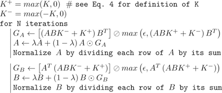
where ☉ denotes the Hadamard product (entry-wise matrix multiplication) and ⊘ denotes the entry-wise matrix division. We set the stabilizer λ to 0.05, ɛ = 10⁻¹⁶, and N=5000 as our approach always converged before that.

In Section 2.1, we derived a robust version of the algorithm by omitting squaring the L₂-norm. Applying the same strategy to Eq. (5) and turning the optimization into an iteratively re-weighted least-square optimization [7] changes the definition of G_A and G_B in the previous algorithm to

$$G_A\leftarrow \left[S\left(AB{K}^{-}+K^{+}\right)B^T\right]\oslash \hspace{0.17em}max\left(ϵ,S\left(AB{K}^{+}+K^{-}\right)B^T\right)$$ (6)

$$G_B\leftarrow \left[A^{T}S\left(AB{K}^{-}+K^{+}\right)\right]\oslash \hspace{0.17em}max\left(ϵ,A^{T}S\left(AB{K}^{+}+K^{-}\right)\right)$$ (7)

where the weight matrix S is initialized by the identity I and updated via

$$S\leftarrow Diag\left({\left(\left(X-ABX\right){\left(X-ABX\right)}^T\right)}_{i,i}^{\hspace{0.17em}\hspace{0.17em}\hspace{0.17em}\hspace{0.17em}\hspace{0.17em}-1/2}\right)$$ (8)

at each iteration. Using instead the Huber norm in Eq. (5), the previous computation of G_A and G_B stay the same but the update rule for S changes to

$$S\leftarrow Diag\left(\frac{{\Vert {\left(\left(X-ABX\right){\left(X-ABX\right)}^T\right)}_{i,i}\Vert }_H}{{\left(\left(X-ABX\right){\left(X-ABX\right)}^T\right)}_{i,i}}\right).$$ (9)

We greatly reduced the computational cost associated with Eq. (8) and (9) by reformulating them like Eq. (3) to use Gramian matrices in our implementation.

3. Experiments

3.1. Data Pre-processing

The analysis focused on resting-state fMRI scans acquired for 281 individuals part of a study investigating the effects of alcohol consumption on the brain [14]. Preprocessing of each scan included motion correction [10], band-passed filtering between 0.01 and 0.1 Hz, registering to an atlas [17], and applying spatial Gaussian smoothing of 5.0 mm FWHM. The 111 regions of interest of the atlas [17] were used to define an average connectivity matrix, which was further reduced to correlations among the 17 brain areas shown in Fig. (2) by applying the Louvain method [2]. These areas were used to define the final functional correlations that were z-transformed [6]. For each study participant, the total alcohol consumption during life was determined based on self-reported consumption and ranged between 0 and 4718 kg. We also considered sex and HIV status, which are known to impact brain structure significantly [14, 15].

Fig. 2.

The 17 brain areas determined by Louvain method.

3.2. Synthetic Experiments

The synthetic data set was generated from three real correlation matrices and was used to a) compare standard, robust, and Huber loss implementations of the convex hull optimization (Section 2.2) and b) test the ability of the three different DPM implementations to fit challenging nonlinear trends (Section 2.1).

The first synthetic data set consists of 75 normal matrices, which are generated by randomly and uniformly sampling from the 2D-simplex formed by the 3 selected matrices. Each of the three implementations is applied to this data set 10 times, where each time the methods use a different random initialization. For each run and iteration, the Squared Euclidean error (see Eq. (5)) is recorded, which is summarized in Fig. (3) A showing that all three implementations converged by 1500 iterations. Next, we repeat the entire analysis adding 25 outlier matrices to the data set. An outlier is created by the convex combination of a normal matrix (with weight 0.2) and the correlation matrix (weight: 0.8) obtained for random time series of two time points sampled from N (0, 1). We then report the error separately for the normal (Fig (3 B)) and the outlier matrices (Fig (3 C)). As expected, the standard approach performs very well when just trained on normal matrices (Fig. (3 A)), but the reconstruction error for normal matrices greatly increases when including outliers (Fig. (3 B)) as it also optimizes the loss function for them (Fig. (3 C)). In contrast, robust and Huber loss implementations largely ignore outliers. The Huber loss implementation is the only one that generates optimal convex hulls on datasets with and without outliers.

Fig. 3.

(A) Squared Euclidean error (see Eq. 5) when fitted on the normal samples only, (B) error in fitting normals when the fitting was based on 25% of the samples being outliers, and (C) the error associated with the outliers.

To test the abilities of the DPM implementations to fit nonlinear trends, we generated 4 different data sets. Each data set contained three groups of normal matrices. For each group, we randomly sampled three locations in the 2D simplex to define a quadratic B-spline. For each B-spline, we generated 50 correlation matrices by randomly sampling locations along the curve and computing the convex combination accordingly. The resulting matrices were corrupted by adding Gaussian noise N(0, 0.1) and projecting them back onto the simplex. The factors describing each matrix were then the group assignment and the relative location on the B-spline (between 0 and 1). After creating four data sets containing normal samples, we derived from each data set one corrupted by 10%, 20%, and 25%. For each group, a cluster of outliers was created around a random location on the 2D simplex by selecting a fraction of the normal samples at random and then replacing their matrices with the one generated with respect to that location. The three DPM variants were then applied to the resulting 16 datasets. For each data set and implementation, DPM was run using the previously described factors as input, 10000 iterations, and a convex hull of 5,10,15,20, or 25 basis matrix. The resulting error scores of the 80 runs per DPM implementation were then summarized in the plot of Fig. (4). As in the previous experiment, robust DPM demonstrated good robustness to outliers compared to the standard approach, and the approach that provided a trade-off between the two was the implementation based on the Huber loss. This quantitative finding is also supported by the 2D simplexes shown in Fig. (4), which reveal that for the dataset with 25% outliers standard DPM was not able to recover the shape of the 3 B-Splines, Huber DPM was better at it, while robust DPM achieved the best results.

Fig. 4.

Predictions of standard, robust and Huber DPM for a data set with 25% of outliers. Large markers are DPM predictions, small ones are training samples, the black dots are the 3 selected real matrices, and the convex hull is shown with black squares. Color brightness increases along the splines. All the results are displayed in the 2-simplex coordinates. The plot to the right summarizes the median prediction error.

4. Connectomes Specific to Sex, HIV, and Alcohol

We applied the 3 DPM implementations (dimension of convex hull: [5,10,25,50,100]) to the entire data set with the continuous factor alcohol consumption and the binary factors sex and HIV status as input. We measured the accuracy of each implementation via Monte-Carlo cross-validation. More specifically, we randomly split our data set into sets of 224 and 57 scans twenty-five times. For each split, we trained the methods using the large set, and we measured the squared Euclidean distance between the matrices in the small set and matrices predicted by the trained models. The results are summarized in Figure (5 A), which revealed that the best DPM was obtained for a convex hull of 5 basis correlation matrices and the Huber loss. The best DPM implementation was also much better than linear, quadratic, and cubic regression models (Figure (5 B)), which predicted the values of the correlation matrices independently for each matrix element.

Fig. 5.

(A) DPM cross-validation error for all the convex hulls and all DPM variants. (B) comparison between DPM and component-wise polynomial regressions.

Fig. (6) shows the connectome generated by DPM and quadratric regression for women with and without HIV that did no drink any alcohol (baseline). The connectomes of both methods agree that the effect of HIV is rather minor in comparison to that of alcohol consumption, whose difference to the baseline is shown in the images to the right. Furthermore, the effect of alcohol consumption is stronger in women with HIV compared to those without HIV and seems to strengthen as alcohol consumption increases; findings echoed by the clinical literature [15]. Disagreement among the methods is about the strength of alcohol consumption effects on brain function, which are more subtle according to connectomes generated by DPM. These more subtle effects also seem more realistic based on the error plots of Fig. (5 B). Cubic regression models (not shown here for the sake of simplicity) predicted unrealistic alcohol effects that were diverging even faster than the quadratic models.

Fig. 6.

Functional connectivity changes induced by alcohol consumption predicted in women with and without HIV, as a function of total lifetime alcohol consumption (in kg). Baseline functional connectivity is shown on the left. Functional connectivity changes induced by alcohol are shown on the right.

5. Conclusion

In this paper, we introduced a new approach to model non-linear changes of the functional connectome with respect to factors, such as brain disorders and alcohol consumption. We described the connectome as a convex combination of basis correlation matrices modeled by deep neural networks. We established the validity of our approach via synthetic experiments. Applied to rs-fMRIs of 281 subjects, we showed that our approach is more accurate than simpler regression approaches and results in factor-dependent connectomes that reveal an effect of alcohol-HIV comorbidity on brain function.

References

- 1.Biswal B, Zerrin Yetkin F, Haughton V, Hyde J: Functional connectivity in the motor cortex of resting human brain using echo-planar mri. Magnetic Resonance in Medicine 34(4), 537–541 (1995) [DOI] [PubMed] [Google Scholar]
- 2.Blondel V, Guillaume JL, Lambiotte R, Lefebvre E: Fast unfolding of communities in large networks. Journal of Statistical Mechanics: Theory and Experiment 2008(10), P10008 (2008) [Google Scholar]
- 3.Chanraud S, Pitel AL, Pfefferbaum A, Sullivan E: Disruption of functional connectivity of the default-mode network in alcoholism. Cerebral Cortex 21(10), 2272–2281 (2011) [DOI] [PMC free article] [PubMed] [Google Scholar]
- 4.Fair DA, Cohen AL, Power JD, Dosenbach NUF, Church JA, Miezin FM, Schlaggar BL, Petersen SE: Functional brain networks develop from a “local to distributed“ organization. PLoS Computational Biology 5(5) (2009) [DOI] [PMC free article] [PubMed] [Google Scholar]
- 5.Fair DA, Dosenbach NUF, Church JA, Cohen AL, Brahmbhatt S, Miezin FM, Barch DM, Raichle ME, Petersen SE, Schlaggar BL: Development of distinct control networks through segregation and integration. Proceedings of the National Academy of Sciences (PNAS) 104(33), 13507–13512 (2007) [DOI] [PMC free article] [PubMed] [Google Scholar]
- 6.Fisher R: Frequency distribution of the values of the correlation coefficient in samples of an indefinitely large population. Biometrika 10(4), 507–521 (1915) [Google Scholar]
- 7.Green P: Iteratively reweighted least squares for maximum likelihood estimation, and some robust and resistant alternatives. Journal of the Royal Statistical Society. Series B (Methodological) 46(2), 149–192 (1984) [Google Scholar]
- 8.Hofmann T, Schölkopf B, Smola A: Kernel methods in machine learning. The Annals of Statistics 36(3), 1171–1220 (2008) [Google Scholar]
- 9.Huber P: Robust estimation of a location parameter. Annals of Statistics 53(1), 73–101 (1964) [Google Scholar]
- 10.Jenkinson M, Bannister P, Brady J, Smith S: Improved optimisation for the robust and accurate linear registration and motion correction of brain images. NeuroImage 17(2), 825–841 (2002) [DOI] [PubMed] [Google Scholar]
- 11.Krizhevsky A, Sutskever I, Hinton G: Imagenet classification with deep convolutional neural networks. Advances in neural information processing systems 25 (2012) [Google Scholar]
- 12.Lee D, Seung H: Algorithms for non-negative matrix factorization. Proceedings of the 2000 Advances in Neural Information Processing Systems Conference pp. 556–562 (2001) [Google Scholar]
- 13.Lundervold A, Lundervold A: An overview of deep learning in medical imaging focusing on mri. Zeitschrift für Medizinische Physik 29(2), 102–127 (2019) [DOI] [PubMed] [Google Scholar]
- 14.Pfefferbaum A, Rogosa D, Rosenbloom M, Chu W, Sassoon S, Kemper C, Deresinski S, Rohlfing T, Zahr N, Sullivan E: Accelerated aging of selective brain structures in human immunodeficiency virus infection. Neurobiology of aging 35(7), 1755–1768 (2014) [DOI] [PMC free article] [PubMed] [Google Scholar]
- 15.Pfefferbaum A, Zahr N, Sassoon S, Kwon D, Pohl K, Sullivan E: Accelerated and premature aging characterizing regional cortical volume loss in human immunodeficiency virus infection: Contributions from alcohol, substance use, and hepatitis c coinfection. Biological Psychiatry: Cognitive Neuroscience and Neuroimaging 3(10), 844–859 (2018) [DOI] [PMC free article] [PubMed] [Google Scholar]
- 16.Rahim M, Thirion B, Varoquaux G: Population shrinkage of covariance (posce) for better individual brain functional-connectivity estimation. Medical Image Analysis 54, 138–148 (2019) [DOI] [PubMed] [Google Scholar]
- 17.Rohlfing T, Zahr N, Sullivan E, Pfefferbaum A: The sri24 multichannel atlas of normal adult human brain structure. Human Brain Mapping 31(5), 798–819 (2014) [DOI] [PMC free article] [PubMed] [Google Scholar]
- 18.Smith SM, Miller KL, Salimi-Khorshidi G, Webster M, Beckmann CF, Nichols TE, Ramsey JD, Woolrich MW: Network modelling methods for fmri. NeuroImage 54, 875–891 (2011) [DOI] [PubMed] [Google Scholar]
- 19.Vergara V, Liu J, Claus E, Hutchison K, Calhoun V: Alterations of resting state functional network connectivity in the brain of nicotine and alcohol users. NeuroImage 151, 45–54 (2017) [DOI] [PMC free article] [PubMed] [Google Scholar]
- 20.Wen D, Wei Z, Zhou Y, Li G, Zhang X, Han W: Deep learning methods to process fmri data and their application in the diagnosis of cognitive impairment: A brief overview and our opinion. Frontiers in Neuroinformatics 12, Article 23 (2018) [DOI] [PMC free article] [PubMed] [Google Scholar]
- 21.Zhu X, Cortes C, Mathur K, Tomasi D, Momenan R: Model-free functional connectivity and impulsivity correlates of alcohol dependence: a resting-state study. Addiction Biology 22(1), 206–217 (2017) [DOI] [PMC free article] [PubMed] [Google Scholar]