Quantum approximate Bayesian computation for NMR model inference

Abstract

Recent technological advances may lead to the development of small scale quantum computers capable of solving problems that cannot be tackled with classical computers. A limited number of algorithms has been proposed and their relevance to real world problems is a subject of active investigation. Analysis of many-body quantum system is particularly challenging for classical computers due to the exponential scaling of Hilbert space dimension with the number of particles. Hence, solving problems relevant to chemistry and condensed matter physics are expected to be the first successful applications of quantum computers. In this paper, we propose another class of problems from the quantum realm that can be solved efficiently on quantum computers: model inference for nuclear magnetic resonance (NMR) spectroscopy, which is important for biological and medical research. Our results are based on three interconnected studies. Firstly, we use methods from classical machine learning to analyze a dataset of NMR spectra of small molecules. We perform a stochastic neighborhood embedding and identify clusters of spectra, and demonstrate that these clusters are correlated with the covalent structure of the molecules. Secondly, we propose a simple and efficient method, aided by a quantum simulator, to extract the NMR spectrum of any hypothetical molecule described by a parametric Heisenberg model. Thirdly, we propose a simple variational Bayesian inference procedure for extracting Hamiltonian parameters of experimentally relevant NMR spectra.

INTRODUCTION

One of the central challenges for quantum technologies during the last few years has been a search for useful applications of near-term quantum machines [1]. While considerable progress has been achieved in increasing the number of qubits and improving their quality [2, 3], in the near future, we expect the number of reliable gates to be limited by noise and decoherence; the so called Noisy Intermediate-Scale Quantum (NISQ) era. As such, hybrid quantum-classical methods have been proposed to make the best out of the available quantum hardware and supplement it with classical computation. Most notably, there has been the development of the Quantum Approximate Optimization Algorithm (QAOA) [4] and the Variational Quantum Eigensolver (VQE) [5]. Both algorithms use the quantum computer to prepare variational states, some of which might be inaccessible through classical computation, but use a classical computer to update the variational parameters. A number of experiments have already been performed, demonstrating the feasibility of these algorithms [6–8], yet their bearing on real world problems remains unclear. In model-based statistical inference one is often faced with similar problems. For simple models one can find the likelihood and maximize it but for complex models the likelihood is typically intractable [9, 10]. Nuclear magnetic resonance (NMR) spectroscopy is a perfect example: there is a good understanding of the type of model that should be used (see equation (1)) and one only needs to determine the appropriate parameters. However, computing the NMR spectrum for a specific model requires performing computations in the exponentially large Hilbert space, which makes it extremely challenging for classical computers. This feature has been one of the original motivations for proposing NMR as a platform for quantum computing [11]. While it has been shown that no entanglement is present during NMR experiments [12, 13], strong correlations make it classically intractable, i.e. the operator Schmidt rank grows exponentially which for example prohibits efficient representation through tensor networks [14] Its computational power is between classical computation and deterministic quantum computation with pure states [15], which makes it an ideal candidate for hybrid quantum-classical methods. As we argue below, the required initial quantum states can be prepared by low depth circuits and the problem is robuust against decoherence. By simulating the model on a quantum computer, it runs efficiently while the remaining inference part is simply solved on a classical computer. One can think of this as an example of quantum Approximate Bayesian Computation (qABC), putting it in the broader scope of quantum machine learning methods [16]. In contrast to most of the proposed quantum machine learning applications, the present algorithm does not require challenging routines such as amplitude amplification [17, 18] or Harrow-Hassidim-Lloyd (HHL) algorithm [19].

NMR-SPECTROSCOPY

NMR spectroscopy is a spectroscopic technique which is sensitive to local magnetic fields around atomic nuclei. Typically, samples are placed in a high magnetic field while driving RF-transitions between the nuclear magnetic states of the system. Since these transitions are affected by the intramolecular magnetic fields around the atom and the interaction between the different nuclear spins, one can infer details about the electronic and thus chemical structure of a molecule in this way. One of the main advantages of NMR is that it is non-destructive, in contrast to, for example, X-ray crystallography or mass spectrometry. This makes NMR one of the most powerful analytical techniques available to biology [20], as it is suited for in vivo and in vitro studies [21]. NMR can, for example, be used for identifying and quantifying small molecules in biological samples (serum, cerebral fluid, etc.) [22–24]. On the other hand, NMR experiments have limited spectral resolution and as such face the challenge of interpreting the data, since extracted information is quite convoluted. We only directly observe the magnetic spectrum of a biological sample, whereas our goal is to learn the underlying microscopic Hamiltonian and ultimately identify and quantify the chemical compounds. While this inference is tractable for small molecules, it quickly becomes problematic, making inference a slow and error-prone procedure [25]. The analysis can be simplified by incorporating a priori spectral information in the parametric model [26]. For that purpose, considerable attention has been devoted to determining NMR model parameters for relevant metabolites such as those found in plasma, cerebrospinal fluid and mammalian brains [27–33].

In what follows we will be concerned with 1D proton NMR but generalization to other situations are straightforward. For liquid ¹H-NMR, a Heisenberg Hamiltonian

$$H(\theta )=\sum _{i,j}{J}_{ij}{S}_i\cdot S_j+\sum _i{h}_i{S}_j^x,$$ (1)

yields a reasonable effective description for the nuclear spins, where θ explicitly denotes the dependence of the Hamiltonian on its parameters θ = {J_ij, h}. Here J_ij encodes the interaction between the nuclear spins S and h_i is the effective local magnetic field. Note that this Hamiltonian contains two essential approximations (i) the interactions are chosen to SU(2) invariant and (ii) the local magnetic fields – called chemical shifts in the NMR literature – are unidirectional. The rationale for the latter is that most of these local magnetic fields are caused by diamagnetic screening due to electronic currents induced by the large external magnetic field. This field will tend to oppose the external field and hence be largely uniaxial. For liquid state NMR, the rapid tumbling of the molecules averages out the dipar coupling between the nuclei, approximately resulting in isotropic exchange interactions between nuclear spins [34]. The fact that the interactions are rotationally invariant, allows us to remove the average (external) field from the Hamiltonian, i.e. $S_{tot}^x={\sum }_i{S}_i^x$ commutes with Hamiltonian (1) and will therefore only shift the NMR spectrum.

Within linear response the evolution of the system subject to a radio frequency z-magnetic field is determined by the response function:

$$S(t\mid \theta )=\text{Tr }\left[e^{iH(\theta )t}{S}_{tot}^z{e}^{-iH(\theta )t}{S}_{tot}^z{\rho }_0\right],$$ (2)

where ρ₀ denotes the initial density matrix of the system and $S_{tot}^z={\sum }_i{S}_i^z$. The measured spectrum is simply given by:

$$A(\omega \mid \theta )=\text{Re}{\int }_0^{\infty }dt{e}^{i\omega t-\gamma t}S(t\mid \theta ),$$ (3)

where γ is the effective decoherence rate. For room temperature ¹H-NMR, the initial density matrix can be taken to be an infinite temperature state, i.e.

$${\rho }_0\approx \frac{\mathbb{1}}{\text{Tr }[\mathbb{1}]}.$$ (4)

Indeed, even a 20 T magnetic field will only lead to a bare proton resonance frequency of about 900 MHz. In contrast, room temperature is about 40 THz, so for all practical purposes we can consider it equally likely for the spin to be in the excited state or in the ground state. Chemical shifts h_i are of the order of a few parts per million, resulting in local energy shifts of a few kHz, while the coupling or interaction strength J is of the order of a few Hz. Despite these low frequencies and the high temperature of the system, one can typically still infer the parameters due to the small decoherence rate of the proton nuclear spin. Due to the absence of a magnetic quadrupole moment, the protons do not decohere from the electric dipole fluctuations caused by the surrounding water molecules. This gives the proton nuclear spin a coherence time of the order of seconds to tens of seconds, sufficiently long to create some correlations between the various spins. The remaining part of this work is concerned with the question of how to infer the model parameters J_ij and h_i of our effective Hamiltonian (1) from a measured spectrum (3).

CLUSTERING

Given real NMR data, summarized by the experimentally acquired spectrum $\mathcal{A}(\omega )$, our goal, in general, is to learn a parametrized generative model which explains how this NMR data is generated. Fortunately, we have a good idea about the physics which allows us to write down a model, i.e. expressions (3), that is close to reality thereby ensuring a small misspecification error. The drawback however is that the model is analytically intractable and becomes increasingly complex to simulate with increasing number of spins. In the next section we will discuss how to alleviate this problem by using a programmable quantum simulator to simulate the problem instead. Even if we can simulate our model (3), we still have to find a reliable and robust way to estimate the parameters θ. Physical molecules have far from typical parameters θ, see SI for a mathematical description. After all, if they do not, how could we infer any structural information out of the spectrum? To extract NMR spectral features, we first perform unsupervised learning on a dataset containing 69 small organic molecules, all composed out of 4 ¹H-atoms, observable in NMR 1D-¹H experiments. Their effective Hamiltonian parameters θ have previously been determined, which provides us with a labeled dataset to test our procedure. Furthermore, by only using the spectra themselves, we can use any relevant information as an initial prior for inference on unknown molecules. The dataset was compiled using the GISSMO library [30, 31, 35]. In order to extract the structure in the dataset, we perform a t-distributed stochastic neighborhood embedding (t-SNE) [36, 37] to visualize the data in 2 dimensions. Fig 1–B, shows the 2-dimensional t-SNE embedding of the dataset based on the Hellinger distance shown in Fig. 1–A, a detailed comparison of different metrics is presented in the SI. The colorscale in panel B shows the inverse participation ratio of each sample, $\text{IPR}={\int }_{-\infty }^{\infty }\text{d}\omega A(\omega \mid \theta )/{\int }_{-\infty }^{\infty }\text{d}\omega A^2(\omega \mid \theta )$,, a measure for the total number of transitions that contribute to the spectrum. At least 4 well defined clusters are identified, density-based spatial clustering of applications with noise (DBSCAN) [38] was used to perform the clustering. Using the clusters as indicated in Fig. 1–B, we can sort the molecules per cluster and have a look at the spectra. The sorted distance matrix is shown in Fig. 2–A, it clearly shows we managed to find most of the structures in the system. In fact a closer look at the spectra of each of the clusters indeed reveals they are all very similar. Fig. 2–B shows a representative spectrum for each of the clusters, as expected the IPR goes up if we go from cluster one to cluster four. All spectra in cluster 1 have the property of containing two large peaks and two small peaks, where the larger peak is about three times higher than the small peak. This is indicative of molecules with a methyl group (CH3) with its protons coupled with a methine proton (CH). One example of such structures can be seen in acetaldehyde oxime (BMRB ID [39]: bmse000467) (as shown to the left in Fig. 2–B). The fact that the 3 protons are equivalent results in the 3:1 ratio of the peaks. Molecules from cluster 2 have are highly symmetric and have two pairs of two methine protons (CH) where the protons are on neighboring carbon atoms. The symmetry in the molecule makes the spectrum highly degenerate. In contrast, cluster 3 has molecules where there are two neighboring methylene groups (CH2). The interacting splitting causes a spectrum as shown in Fig. 2–B. Finally, cluster 4 has four inequivalent protons with different chemical shifts and interactions between them. As a results, there is a plethora of possible transitions and the spectrum has an erratic form such as shown in Fig. 2–B. In that sense, cluster 4 is most like a disordered quantum spin chain.

Figure 1. Clustering.

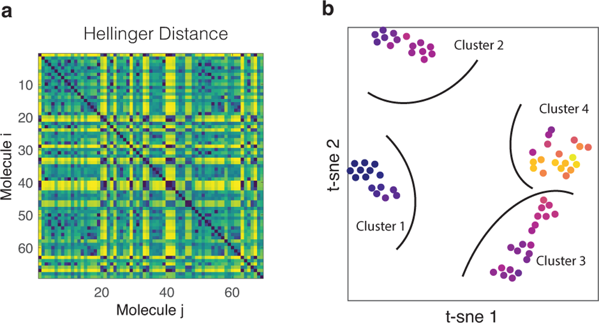
In order to identify whether naturally occurring molecules have some atypical NMR spectrum, we perform a clustering analysis. In panel–A we show the distance between the various NMR spectra, where the Bhattacharyya coefficient is used to measure similarity. To obtain a meaningful comparison, spectra are shifted and scaled such that they are all centered around the same frequency and have the same bandwidth. To extract clusters we perform a t-SNE shown in panel–B with perplexity of 10; which is chosen because it has minimal Kullback-Leibler (KL) loss, i.e. the KL-loss was 0.145.

Figure 2. NMR Spectra.

By clustering the molecules according to the Hellinger distance t-SNE clusters we can reorganize the distance matrix as shown in panel A. For each of the clusters, we look at the different spectra, which indeed show great similarity. A representative spectrum for each of the clusters is shown in panel B, where the spectra are labeled according to the t-SNE clusters shown in Fig. 1–B. In addition, we show an example small molecule out of this cluster next to the associated spectrum. The atoms and interactions responsible for the shown portions of the spectra are indicated in blue and red arrows respectively.

Given a new spectrum of an unknown molecule we can find out whether the molecule belongs to any of the identified molecular sub-structures, i.e. by computing the mean Hellinger distance to each of the identifed clusters one can robustly classify the spectra. In the supplemental information we present results in which we randomly choose 39 samples and consider those as clustered, while we use the other 30 samples to test the procedure. Samples that belong to cluster 1 and 2 are always correct classified. One sample from cluster 4 was misclassified for cluster 3. Since we know the spin matrix θ_i for each of the molecules in the dataset, we have a rough estimate of what the Hamiltonian parameters are and where the protons are located with respect to each other. However, there is still a lot of fine structure within clusters, in particular in clusters 3 and 4, as can be seen in Fig. 2–A. In what remains, we are concerned with finding an algorithm to further improve the Hamiltonian parameter estimation.

QUANTUM COMPUTATION

While our model is microscopically motivated, thereby capturing the spectra very well and allowing for a physical interpretation of the model parameters, it has the drawback that, unlike simple models such as Lorentzian mixture models [40, 41], there is no analytic form for the spectrum in terms of the model parameters. Moreover, even simulating the model becomes increasingly complex when the number of spins increase. Before we solve the inference problem, let us present an efficient method to extract the simulated NMR spectrum on a quantum simulator-computer. The basic task is to extract the spectrum (3) by measuring (2). Recall that we work at infinite temperature, hence by inserting an eigen-basis of the total z-magnetization $S_{tot}^z={\sum }_j{m}_j|z_j\rangle \langle z_j|$, we find

$$S(t\mid \theta )=\sum _{i,j}{m}_i{m}_j{P}_t(i\mid j,\theta )P_0(j),$$ (5)

with the transition probability P_t(i|j, θ) = |〈z_i|U_θ(t)|z_j〉|², initial distribution P₀(j) = 2^−N and m_j is the total z-magnetization in the eigenstate |z_j〉. Consequently, we can extract the spectrum by initializing our system in a product state of z-polarized states after which we quench the system to evolve under U_θ(t) generated by Hamiltonian H(θ), and then finally performing a projective measurement in the z-basis again at time t. By repeating the procedure by uniformly sampling initial eigenstates and estimating the product of the initial and final magnetization m_im_j, one obtains an estimate of S(t|θ), see Fig. 3. Note that, at this stage, the problem is entirely classical and all quantum physics is hidden in the transition probablity P_t(i|j, θ). It is the intractability of this transition probability that forms the basis of recent quanum supremacy experiments [42].

Figure 3. Method overview.

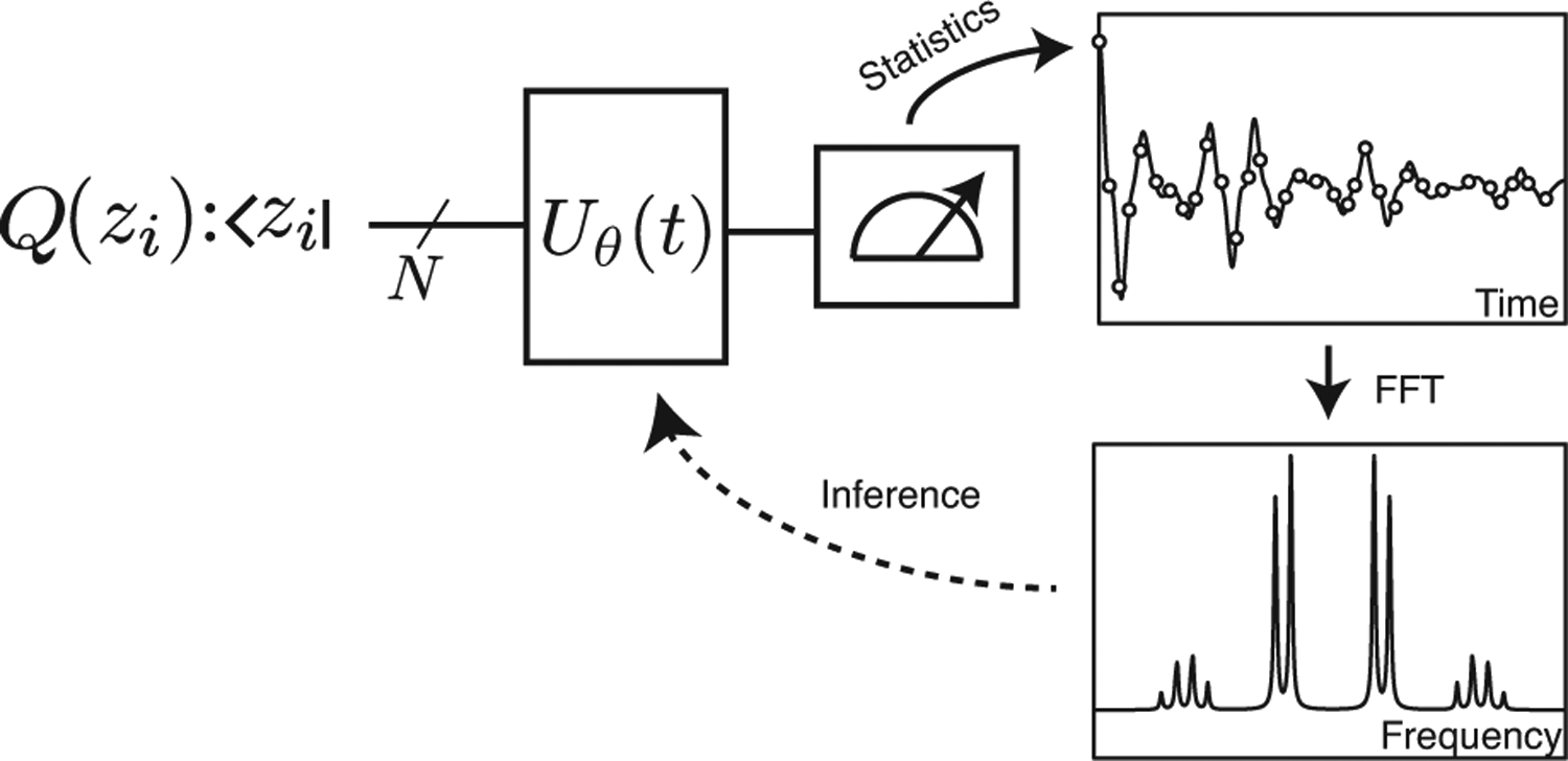
Take a product state |z_i〉 with a given total magnetization m_i, according to Q₀(j). The latter can be choosen to minimze the variance of the estimand. After this initial preparation, we evolve the state under the Hamiltonian H(θ) and measure the project back onto the z-basis at time t. By applying a fast Fourier transform to the estimate S(t|θ), one obtains the spectrum which can be used to infer the parameters of the Hamiltonian.

In contrast to the latter, we are only interested in estimating a simple statistic, namely the average m_im_j. Note that this quantity is bounded by N²/4, hence according to Hoeffding’s inequality one needs to sample at most O(N⁴/ϵ²) times to get an precision of ϵ on S(t|θ). At present, the structure of Eq. (5) allows one to bound the variance of m_im_j by 3(N/4)², such that O(N²/ϵ²) would suffice. As shown in detail in the SI, one can in general not improve on this scaling with N unless one uses additional structure of the transition probability P_t. At short times one for example benefits from importance sampling. While we have no control over the transition probability P_t, we can control the initial probability out of which we sample states, as long as those states are easy to prepare. Since (5) is diagonal in the z-basis, it’s sufficient to consider sampling product states in z-basis, i.e. one can equivalently write the response function as:

$$S(t\mid \theta )=\sum _{i,j}\left(\frac{m_i{m}_j{P}_0(j)}{Q_0(j)}\right)P_t(i\mid j,\theta )Q_0(j),$$ (6)

where Q₀ is the distribution from which we sample. By minimizing the variance of estimand r = m_im_jP₀/Q₀, one obtains an optimal sampling distribution. The true optimal depends on time through P_t and since this is unknown to us, we must settle for a good, albeit suboptimal, distribution Q₀. Various approximations might be considered, the distribution

$$Q_0(j)=\frac{4}{N}\frac{m_j^2}{2^N},$$ (7)

is particularly interesting because it gives zero variance for r the t = 0 and at any other time the variance is smaller than (N/4)². Consequently we can estimate S(t|θ) with precision ϵ by taking at most O(N²/ϵ²) samples. Given the finite decoherence rate γ and the fact that the energy bandwidth of the many-body spectrum scales linearly with N, one needs to measure S(t|θ) at worst in time steps of the order of 1/N up to a time that scales as 1/γ. One thus has to repeat the entire circuit at worst O(N³/ϵ²) times. Furthermore, if the time-evolution is implemented as an analog simulation this takes a time of O(1/γ). The gate complexity is at worst a factor N² more because one, at worst, has to implement a Heisenberg interaction between all possible qubits, yielding O(N²/γ). Note that these are worst case scalings, for an extensive spectrum one actually expects linear scaling of the gate complexity with N and typical transition happen between states with only differ by an energy of O(1) such that the typical sampling complexity is only quadratic with N.

VARIATIONAL BAYESIAN INFERENCE

Now that we have a procedure of efficiently obtaining spectra of hypothetical molecules, how do we solve the inference problem? The standard approach would be to do maximum likelihood estimation of the parameters given the experimental spectrum or minimize one of the aforementioned cost functions. This cannot be done analytically and the problem can clearly be highly non-convex. We thus require a method to numerically minimize the error; gradient descend seems an obvious choice but is not well suited for this task. First of all there is the obvious problem that additional measurements will need to performed to estmate the gradients. Those estimates are not easy to obtain since they require measuring three-point correlators in time. Moreover, using a quantum simulator, one only obtains a statistical estimate of the cost function and its gradient; since we only perform a finite number of measurements. In order to move down the optimization landscape we thus need to resolve the signal from the noise, meaning gradients have to be sufficiently large to be resolved. However, we find extremely small gradients for this problem. Taking for example the Hellinger distance, D_H, used to construct Fig. (1), we find the gradient satisfies

$$|{\partial }_{\theta }{D}_H^2|=\left|\int \frac{\text{d}\omega }{2\pi }\sqrt{\frac{\mathcal{A}(\omega )}{A(\omega \mid \theta )}}{\partial }_{\theta }A(\omega \mid \theta )\right|\le \sqrt{I_{\theta \theta }},$$ (8)

where I_θθ is the diagonal component of the Fisher information. The bound simply follows from Cauchy-Schwarz inequality. As shown in the SI, the Fisher information, even for the optimal values, is very small; typically of the order 10⁻⁴ − 10⁻⁶ for our 4 spin molecules. We are thus in a situation of a very shallow rough optimization landscape. The problem is of similar origin as the vanishing gradient problem in quantum neural networks [43]. A gradient free method seems advisable. Here we adopt a Bayesian approach to update our estimated parameters. Alternative approaches, such as the DIRECT method addopted in Ref. [44], are expected to work as well. More research on the structure of the optimzation landscape is required to understand the hardness of this inference problem. Recall Bayes theorem, in the current notation, reads:

$$P(\theta \mid \omega )=\frac{A(\omega \mid \theta )P(\theta )}{A(\omega )},$$ (9)

where P(θ|ω) is the conditional probability to have parameters θ given that we see spectral weight at frequency ω, A(ω|θ) is the NMR spectrum for fixed parameters θ, P(θ) is the probability to have parameters θ and A(ω) is the marginal NMR spectrum averaged over all θ. If we acquire some data, say a new spectrum $\mathcal{A}(\omega )$ and we have some prior belief about the distribution P(θ), we can use it to update our belief about the distribution of the parameters, i.e.

$$P_{i+1}(\theta )=\int \frac{\text{d}\omega }{2\pi }\mathcal{A}(\omega )\frac{A(\omega \mid \theta )}{A_i(\omega )}{P}_i(\theta ),$$ (10)

with A_i(ω) = ∫ dθA(ω|θ)P_i(θ). Note that the above rule indeed conserves positivity and normalization. Moreover, it simply reweights the prior distribution with some weight

$$w_i(\theta )=\int \frac{\text{d}\omega }{2\pi }\mathcal{A}(\omega )\frac{A(\omega \mid \theta )}{A_i(\omega )},$$ (11)

that is directly related to the log-likelihood, since Jensen inequality gives:

$$\text{log}\left(w_i(\theta )\right)\ge \int \frac{\text{d}\omega }{2\pi }\mathcal{A}(\omega )\text{ log}\frac{A(\omega \mid \theta )}{A_i(\omega )}=\mathcal{L}(\theta )+c,$$ (12)

where $\mathcal{L}(\theta )$ is the log-likehood and c is a constant independent of θ. Consequently, iterating expression (10) is expected to converge to a distribution of parameters which is highly peaked around the maximum likelihood estimate. While it avoids the use of any gradients, it requires us to sample from the current parameter distribution P_i(θ). This by itself could become intractable and so we make an additional approximation. In order to be able to sample from the parameter distribution, we approximate it by a normal distribution at every step. That is, given that we have obtained some Monte Carlo samples out of P_i(θ), we can estimate all the weights w_i(θ) by simply simulating the model and obtaining A(ω|θ_i) for all the samples. Next, we approximate P_i+1(θ) with a normal distribution that is a close as possible to it, i.e. has minimal KL-distance. The latter is simply the distribution with the same sample mean and covariance as P_i+1(θ). We use an atomic prior, $P_0(\theta )={\sum }_i\frac{1}{N_s}\delta \left(\theta -{\theta }_i\right)$, consisting of all the samples that belong to the same cluster to which the spectrum is identified to belong. The result of this procedure for some randomly chosen test molecules is shown in Fig. 4. We observe steady, albeit noisy, convergence of the molecular spectra. Convergence is limited by three factors, i.e. (i) shot noise from the quantum measurements, (ii) sampling noise from the Monte Carlo procedure and (iii) the Gaussian variational approximation. While both noise sources can be made smaller by using more computational resources, more advanced methods might ultimately be needed.

Figure 4. Inference.

For each of the clusters, labeled according to Fig. 2, we investigate the convergence of the parameter inference in our variational Bayesian inference scheme by looking at the total variation distance between the spectra. The dashed line indicates the shot noise limit, set by the finite number of acquired quantum measurements.

SUMMARY AND OUTLOOK

Here we have presented a method to improve model inference for NMR with relatively modest amount of quantum resources. Similar to generic generative models such as Boltzmann machines, for which a more efficient quantum version has been constructed [45, 46], we have constructed an application specific model from which a quantum machine can sample more efficiently than a classical computer. Model parameters are determined through a variational Bayesian approach with an informative prior, constructed by applying t-SNE to a dataset of small molecules. As a consequence of the noisy nature of the generative model, as well as the absence of significant gradients, both the initial bias as well as the derivative free nature of Bayesian inference are crucial to tackling the problem. This situation, however, is generic to any hybrid quantum-classical setting that is sufficiently complicated. A similar approach might thus be useful to improve convergence of QAOA or VQE, e.g.heuristic optimization strategies for QAOA have been developed in Ref. [47]. Both the classical and quantum part of our approach can be extended further. On the quantum side, one can envision developing more efficient approaches for computing the spectra; trading computational time for extra quantum resources. On the classical side, improvements on the inference algorithm might be possible by combining or extending the variational method with Hamiltonian Monte Carlo techniques [48].

It is interesting to extend our technique to other types of experiments. NMR is hardly the only problem where one performs inference on spectroscopic data. For example, one can imagine combining resonant inelastic X-ray scattering (RIXS) data from strongly correlated electron systems [49], with Fermi-Hubbard simulators based on ultracold atoms [50, 51]. Currently, RIXS data is analyzed by performing numerical studies of small clusters on classical computers (see Ref. [52] for review). A DMFT-based hybrid algorithm was recently proposed in [53]. With cold atoms in optical lattices one may be able to create larger systems and study their non-equilibrium dynamics corresponding to RIXS spectroscopy.

References

- [1].Preskill J, Quantum 2, 79 (2018). [Google Scholar]
- [2].Bernien H, Schwartz S, Keesling A, Levine H,Omran A, Pichler H, Choi S, Zibrov AS, Endres M, Greiner M, Vuletić V, and Lukin MD, Nature 551, 579 EP (2017). [DOI] [PubMed] [Google Scholar]
- [3].Friis N, Marty O, Maier C, Hempel C, Holzäpfel M, Jurcevic P, Plenio MB, Huber M, Roos C, Blatt R, and Lanyon B, Phys. Rev. X 8, 021012 (2018). [Google Scholar]
- [4].Farhi E, Goldstone J, and Gutmann S, “A quantum approximate optimization algorithm,” (2014), arXiv:1411.4028. [Google Scholar]
- [5].Peruzzo A, McClean J, Shadbolt P, Yung M-H, Zhou X-Q, Love PJ, Aspuru-Guzik A, and O’Brien JL, Nature Communications 5, 4213 EP (2014). [DOI] [PMC free article] [PubMed] [Google Scholar]
- [6].Kokail C, Maier C, van Bijnen R, Brydges T, Joshi MK, Jurcevic P, Muschik CA, Silvi P, Blatt R, Roos CF, and Zoller P, Nature 569, 355 (2019). [DOI] [PubMed] [Google Scholar]
- [7].Kandala A, Mezzacapo A, Temme K, Takita M,Brink M, Chow JM, and Gambetta JM, Nature 549, 242 EP (2017). [DOI] [PubMed] [Google Scholar]
- [8].Colless JI, Ramasesh VV, Dahlen D, Blok MS,Kimchi-Schwartz ME, McClean JR, Carter J, de Jong WA, and Siddiqi I, Phys. Rev. X 8, 011021 (2018). [Google Scholar]
- [9].Diggle PJ and Gratton RJ, Journal of the Royal Statistical Society, Series B: Methodological 46, 193 (1984). [Google Scholar]
- [10].Beaumont MA, Zhang W, and Balding DJ, Genetics 162, 2025 (2002), https://www.genetics.org/content/162/4/2025.full.pdf. [DOI] [PMC free article] [PubMed] [Google Scholar]
- [11].Gershenfeld NA and Chuang IL, Science 275, 350 (1997). [DOI] [PubMed] [Google Scholar]
- [12].Braunstein SL, Caves CM, Jozsa R,Linden N, Popescu S, and Schack R, Phys. Rev. Lett 83, 1054 (1999). [Google Scholar]
- [13].Menicucci NC and Caves CM, Phys. Rev. Lett 88, 167901 (2002). [DOI] [PubMed] [Google Scholar]
- [14].Datta A and Vidal G, Phys. Rev. A 75, 042310 (2007). [Google Scholar]
- [15].Knill E and Laflamme R, Phys. Rev. Lett 81, 5672 (1998). [Google Scholar]
- [16].Biamonte J, Wittek P, Pancotti N, Rebentrost P,Wiebe N, and Lloyd S, Nature 549, 195 EP (2017). [DOI] [PubMed] [Google Scholar]
- [17].Brassard G and Hoyer P, in Proceedings of the Fifth Israeli Symposium on Theory of Computing and Systems (1997) pp.12–23. [Google Scholar]
- [18].Grover LK, Phys. Rev. Lett 80, 4329 (1998). [Google Scholar]
- [19].Harrow AW, Hassidim A, and Lloyd S, Phys. Rev. Lett 103, 150502 (2009). [DOI] [PubMed] [Google Scholar]
- [20].Bothwell JHF and Griffin JL, Biological Reviews 86, 493 (2011), https://onlinelibrary.wiley.com/doi/pdf/10.1111/j.1469-185X.2010.00157.x. [DOI] [PubMed] [Google Scholar]
- [21].Hwang J-H and Choi CS, Experimental &Amp; Molecular Medicine 47, e139 EP (2015). [DOI] [PMC free article] [PubMed] [Google Scholar]
- [22].Beckonert O, Keun HC, Ebbels TMD, Bundy J,Holmes E, Lindon JC, and Nicholson JK, Nature Protocols 2, 2692 EP (2007). [DOI] [PubMed] [Google Scholar]
- [23].Larive CK, Barding GA, and Dinges MM, Analytical Chemistry, Analytical Chemistry 87, 133 (2015). [DOI] [PubMed] [Google Scholar]
- [24].Napolitano J, Lankin DC, McAlpine JB,Niemitz M, Korhonen S-P, Chen S-N, and Pauli GF, The Journal of Organic Chemistry, The Journal of Organic Chemistry 78, 9963 (2013). [DOI] [PMC free article] [PubMed] [Google Scholar]
- [25].Ravanbakhsh S, Liu P, Bjordahl TC, Mandal R, Grant JR, Wilson M, Eisner R, Sinelnikov I, Hu X, Luchinat C, Greiner R, and Wishart DS, PLOS ONE 10, 1 (2015). [DOI] [PMC free article] [PubMed] [Google Scholar]
- [26].De Graaf AA and Boveé WMMJ, Magnetic Resonance in Medicine 15, 305 (1990). [DOI] [PubMed] [Google Scholar]
- [27].Wevers RA, Engelke U, and Heerschap A, Clinical Chemistry 40, 1245 (1994), http://clinchem.aaccjnls.org/content/40/7/1245.full.pdf. [PubMed] [Google Scholar]
- [28].Wevers RA, Engelke U, Wendel U, de Jong JG, Gabreëls FJ, and Heerschap A, Clinical Chemistry 41, 744 (1995), http://clinchem.aaccjnls.org/content/41/5/744.full.pdf. [PubMed] [Google Scholar]
- [29].Govindaraju V, Young K, and Maudsley AA, NMR in Biomedicine 13, 129 (2000). [DOI] [PubMed] [Google Scholar]
- [30].Dashti H, Wedell JR, Westler WM, Tonelli M,Aceti D, Amarasinghe GK, Markley JL, and Eghbalnia HR, Analytical Chemistry, Analytical Chemistry 90, 10646 (2018). [DOI] [PMC free article] [PubMed] [Google Scholar]
- [31].Dashti H, Westler WM, Tonelli M, Wedell JR, Markley JL, and Eghbalnia HR, Analytical Chemistry, Analytical Chemistry 89, 12201 (2017). [DOI] [PMC free article] [PubMed] [Google Scholar]
- [32].Pickard CJ and Mauri F, Phys. Rev. B 63, 245101 (2001). [DOI] [PubMed] [Google Scholar]
- [33].Paruzzo FM, Hofstetter A, Musil F,De S, Ceriotti M, and Emsley L, Nature Communications 9, 4501 (2018). [DOI] [PMC free article] [PubMed] [Google Scholar]
- [34].Levitt MH, Spin Dynamics: Basics of Nuclear Magnetic Resonance (Wiley, 2008). [Google Scholar]
- [35].Dashti H, “http://gissmo.nmrfam.wisc.edu/,” (2019).
- [36].van der Maaten L and Hinton G, Journal of Machine Learning Research 9, 2579 (2008). [Google Scholar]
- [37].van der Maaten L, “https://lvdmaaten.github.io/tsne/,” (2019).
- [38].Ester M, Kriegel H-P, Sander J, and Xu X (AAAI Press, 1996) pp. 226–231. [Google Scholar]
- [39].Ulrich EL, Akutsu H, Doreleijers JF, Harano Y, Ioannidis YE, Lin J, Livny M, Mading S,Maziuk D, Miller Z, Nakatani E, Schulte CF, Tolmie DE, Kent Wenger R, Yao H, and Markley JL, Nucleic acids research 36, D402 (2008). [DOI] [PMC free article] [PubMed] [Google Scholar]
- [40].Sokolenko S, Jzquel T, Hajjar G, Farjon J, Akoka S, and Giraudeau P, Journal of Magnetic Resonance 298, 91 (2019). [DOI] [PubMed] [Google Scholar]
- [41].Xu K, Marrelec G, Bernard S, and Grimal Q, IEEE Transactions on Signal Processing 67, 4 (2019). [Google Scholar]
- [42].Arute F, Arya K, Babbush R, Bacon D, Bardin JC, Barends R, Biswas R, Boixo S, Brandao FGSL, Buell DA, Burkett B, Chen Y, Chen Z, Chiaro B, Collins R, Courtney W, Dunsworth A, Farhi E, Foxen B, Fowler A, Gidney C, Giustina M, Graff R, Guerin K, Habegger S, Harrigan MP, Hartmann MJ, Ho A, Hoffmann M, Huang T, Humble TS, Isakov SV, Jeffrey E, Jiang Z, Kafri D, Kechedzhi K, Kelly J, Klimov PV, Knysh S, Korotkov A, Kostritsa F, Landhuis D, Lindmark M, Lucero E, Lyakh D, Mandrà S, McClean JR, McEwen M, Megrant A, Mi X, Michielsen K, Mohseni M, Mutus J, Naaman O, Neeley M, Neill C, Niu MY, Ostby E, Petukhov A, Platt JC, Quintana C, Rieffel EG, Roushan P, Rubin NC, Sank D, Satzinger KJ, Smelyanskiy V, Sung KJ, Trevithick MD, Vainsencher A, Villalonga B, White T, Yao ZJ, Yeh P, Zalcman A, Neven H, and Martinis JM, Nature 574, 505 (2019). [DOI] [PubMed] [Google Scholar]
- [43].McClean JR, Boixo S, Smelyanskiy VN, Babbush R, and Neven H, Nature Communications 9, 4812 (2018). [DOI] [PMC free article] [PubMed] [Google Scholar]
- [44].Kokail C, Maier C, van Bijnen R, Brydges T, Joshi MK, Jurcevic P, Muschik CA, Silvi P, Blatt R, Roos CF, and Zoller P, Nature 569, 355 (2019). [DOI] [PubMed] [Google Scholar]
- [45].Kieferová M and Wiebe N, Phys. Rev. A 96, 062327 (2017). [Google Scholar]
- [46].Amin MH, Andriyash E, Rolfe J, Kulchytskyy B, and Melko R, Phys. Rev. X 8, 021050 (2018). [Google Scholar]
- [47].Zhou L, Wang S-T, Choi S, Pichler H, and Lukin MD, “Quantum approximate optimization algorithm: Performance, mechanism, and implementation on near-term devices,” (2018), arXiv:1812.01041. [Google Scholar]
- [48].Neal RM, (2012), arXiv:1206.1901.
- [49].Murakami Y and Ishihara S, eds., Resonant X-Ray Scattering in Correlated Systems (Springer Berlin Heidelberg, 2017). [Google Scholar]
- [50].Hofstetter W, Cirac JI, Zoller P, Demler E, and Lukin MD, Phys. Rev. Lett 89, 220407 (2002). [DOI] [PubMed] [Google Scholar]
- [51].Bloch I, Dalibard J, and Zwerger W, Rev. Mod. Phys 80, 885 (2008). [Google Scholar]
- [52].Ament LJP, van Veenendaal M, Devereaux TP, Hill JP, and van den Brink J, Rev. Mod. Phys 83, 705 (2011). [Google Scholar]
- [53].Kreula JM, García-Álvarez L, Lamata L, Clark SR, Solano E, and Jaksch D, EPJ Quantum Technology 3, 11 (2016). [Google Scholar]
- [54].Mehta P, Bukov M, Wang C-H, Day AG,Richardson C, Fisher CK, and Schwab DJ, Physics Reports 810, 1 (2019), a high-bias, low-variance introduction to Machine Learning for physicists. [DOI] [PMC free article] [PubMed] [Google Scholar]
- [55].Jeffreys H, Proceedings of the Royal Society of London. Series A. Mathematical and Physical Sciences 186, 453 (1946). [DOI] [PubMed] [Google Scholar]
- [56].Waterfall JJ, Casey FP, Gutenkunst RN, Brown KS, Myers CR, Brouwer PW, Elser V, and Sethna JP, Phys. Rev. Lett 97, 150601 (2006). [DOI] [PubMed] [Google Scholar]
- [57].Machta BB, Chachra R, Transtrum MK, and Sethna JP, Science 342, 604 (2013). [DOI] [PubMed] [Google Scholar]
Associated Data
This section collects any data citations, data availability statements, or supplementary materials included in this article.