Measuring subjective probabilities: The effect of response mode on the use of focal responses, validity, and respondents’ evaluations.

Abstract

Subjective probabilities are central to risk assessment, decision making, and risk communication efforts. Surveys measuring probability judgments have traditionally used open-ended response modes, asking participants to generate a response between 0% and 100%. A typical finding is the seemingly excessive use of 50%, perhaps as an expression of “I don’t know.” In an online survey with a nationally representative sample of the Dutch population, we examined the effect of response modes on the use of 50% and other focal responses, predictive validity, and respondents’ survey evaluations. Respondents assessed the probability of dying, getting the flu, and experiencing other health-related events. They were randomly assigned to a traditional open-ended response mode, a visual linear scale ranging from 0% to 100%, or a version of that visual linear scale on which a magnifier emerged after clicking on it. We found that, compared to the open-ended response mode, the visual linear and magnifier scale each reduced the use of 50%, 0%, and 100% responses, especially among respondents with low numeracy. Responses given with each response mode were valid, in terms of significant correlations with health behavior and outcomes. Where differences emerged, the visual scales seemed to have slightly better validity than the open-ended response mode. Both high-numerate and low-numerate respondents’ evaluations of the surveys were highest for the visual linear scale. Our results have implications for subjective probability elicitation and survey design.

summary:

Health surveys that ask probability questions tend to elicit many “fifty-fifty” responses. Such focal responses are less likely with visual response scales than with open-ended response modes.

1. INTRODUCTION

Probability assessment is central to decision making about risk. Risk and decision analysts use probability assessments to build their models, make predictions, and inform decisions. Subjective probabilities also inform the risk communication efforts undertaken by policy makers, health professionals, financial advisers, and other practitioners. The ability to assess probabilities of future outcomes is an essential component of individuals’ decision-making competence (Bruine de Bruin, Parker, & Fischhoff, 2007a; Parker & Fischhoff, 2005).

A growing number of national surveys, including the U.S. Health and Retirement Study, have asked people to assess their subjective probabilities for future events (Hurd, 2009). Although people’s probability judgments may be subject to specific biases (Tversky & Kahneman, 1974), survey research has demonstrated their predictive validity, as seen in significant correlations of reported probabilities with whether or not the predicted event ends up occurring. For example, average survival probabilities reported in the Health and Retirement Study are very close to those presented in life tables and co-vary with self-reported smoking, drinking, health conditions or education in ways that would be expected from studies of actual mortality (Hurd & McGarry, 1995). Moreover, longitudinal panel data from the Health and Retirement Study suggest that individuals’ subjective probabilities predict their actual survival over time (Hurd & McGarry, 2002; Khwaja, Sloan, & Chung, 2007). Similarly, among adolescent participants of the National Longitudinal Study of Youth 1997, judged probabilities for significant life events (such as getting a high school diploma) by age 20 predict their later reports of experiencing those events at age 20 (Bruine de Bruin, Parker, & Fischhoff, 2007b; Fischhoff et al., 2000).

Subjective probabilities have more predictive validity than yes/no questions that ask respondents about their intentions to engage in a behavior (Juster, 1966). In election polls, judged probabilities of voting for different candidates predicted voting behavior and added to the predictive power of verbal responses to traditional polling questions (Delavande & Manski, 2008; Gutsche, Kapteyn, Meijer, & Weerman, 2014). Moreover, female adolescents’ probability judgments for having Chlamydia predicted whether or not they subsequently test positive for that sexually transmitted infection, over and above their self-reports of risk factors, which are typically collected by health care providers (Bruine de Bruin, Downs, Murray, & Fischhoff, 2010). Subjective probability judgments may be correlated to actual events because they allow people to summarize personal information about relevant predictors (Persoskie, 2003).

1.1. A ‘fifty-fifty’ chance

Despite their validity, questions about subjective probabilities tend to consistently elicit a seemingly disproportionate number of 50% responses (Hurd, 2009), in addition to peak use of 0% and 100% (Dominitz & Manski, 1997). While those response patterns may reflect the appeal of round numbers (Manski & Molinari, 2010), it has been posited that 50% is focal because it reflects the verbal phrase “fifty-fifty,” or feeling uncertain about how to respond (Fischhoff & Bruine de Bruin, 1999). Indeed, 50% responses are especially common among respondents with lower levels of numeracy, who tend to struggle more with numbers (Bruine de Bruin, Fischhoff, Millstein, & Halpern-Felsher, 2000). Moreover, 50% is more likely than other probability responses to be explained by respondents as indicating “no one can know the chances” or “no idea” rather than “a good estimate” (Bruine de Bruin & Carman, 2012). Individuals who use those explanations tend to give probability judgments (e.g., for dying in the next 10 years) with lower concurrent validity in terms of correlations with reported experiences (e.g., current health status) (Bruine de Bruin & Carman, 2012).

1.2. The effect of response modes on the use of 50% responses

Traditionally, surveys that have asked respondents for probability assessments, such as the National Longitudinal Study of Youth and the Health and Retirement Study mentioned above, have tended to use open-ended response modes. Such open-ended response modes require respondents to generate their own response options in the range from 0% to 100%. Interviews in which respondents thought out loud while answering open-ended probability questions have shown that the phrase “fifty-fifty” is commonly used to express uncertainty rather than as a numerical response (Fischhoff & Bruine de Bruin, 1999).

Presenting a visual linear scale that shows the numerical response range from 0% to 100% is thought to discourage intrusion from the verbal phrase “fifty-fifty” and reduce the use of non-numerical 50% responses (Fischhoff & Bruine de Bruin, 1999; Bruine de Bruin, Fischbeck, Stiber, & Fischhoff, 2002). Systematic comparisons of open-ended response distributions and visual scale response distributions for the same questions have suggested that respondents who use non-numerical 50% responses with an open-ended question will likely use any number in the 0–100% range when presented with a linear scale (Bruine de Bruin et al., 2002).

However, that previous research did not examine whether the linear scale also reduced the use of other focal responses such as 0% and 100%, or whether the reduction in focal responses held for respondents varying in numeracy. Moreover, its small convenience sample did not provide sufficient statistical power to examine the validity of probability judgments, in terms of correlations with self-reported behaviors. Without such evidence, it remains unclear whether the reduction of focal probability responses that is observed with visual linear scales is increasing response precision and validity, or simply introducing noise. Finally, that research did not provide evidence about respondents’ evaluations of surveys that used the potentially more cumbersome scales. In this paper, we address each of these limitations of the past research.

An additional scale that has been suggested is a visual magnifier scale that enlarges the number of response options in the range from 0–1% (Woloshin, Schwartz, Byram, Fischhoff, & Welch, 2000). This version of the visual magnifier scale has been found to reduce the use of 50%, as compared to traditional open-ended response modes (Fischhoff & Bruine de Bruin, 1999). However, it has been criticized for introducing an artificial response bias towards low probabilities (Gurmankin, Helweg-Larsen, Armstrong, Kimmel, & Volpp, 2005).

Today’s web-based surveys can avoid such artificial response bias by first asking respondents to provide an answer on a traditional visual linear scale, and presenting respondents who give answers between 0% and 1% with a follow-up question that magnifies that range. Doing so has been shown to reduce the use of 0%, increase the resolution of responses in the 0–1% range, and improve predictions of attitudes and self-reported behaviors (Bruine de Bruin, Parker, & Maurer, 2011). Hence, this two-step procedure, which allows respondents to give more precise responses to questions about low-probability events, tends to improve the validity of judgments of low-probability events rather than to simply add noise (Bruine de Bruin et al., 2011). The two-step procedure shows promise for allowing respondents to give more precise responses in the entire 0–100% response range, by presenting them with visual scales.

1.3. Research questions

We had the unique opportunity to randomly assign a large national sample of Dutch residents to judging probabilities for health outcomes while using an open-ended response mode, a visual linear scale ranging from 0% to 100% (Figure 1A), or a two-step procedure involving a visual linear scale followed by an added magnifier over the selected response (henceforth the visual magnifier scale; Figure 1B). Our research questions asked whether, as compared to the traditional open-ended response mode, the visual linear scale and the visual magnifier scale affected low-numerate and high-numerate respondents’ (1) use of 50%, 0%, and 100% probability responses, (2) response validity, as seen in correlations of judged probabilities with reported health behaviors and outcomes, and (3) evaluations of the quality of the survey.

Figure 1:

Sample screen shots showing (A) the visual linear scale (after clicking on 74%), and (B) the visual magnifier scale (after clicking on 49.93%).

2. METHOD

2.1. Sample

2.1.1. Initial survey.

We recruited our sample through the Longitudinal Internet Studies for the Social Sciences (LISS) panel (http://www.lissdata.nl), which includes households that were randomly selected from the Netherlands’ population register, as well as a refreshment sample recruited to improve representativeness. Invited households were offered a computer or an internet connection if they did not already have one. Panel members completed monthly surveys in the Dutch language, and received 15 Euros per hour for their participation.

A total of 8143 panel members were invited to participate in our survey on the effect of response modes on reported subjective probabilities. Of those, 5817 completed it, for a response rate of 71.4%. We excluded 134 respondents because their browsers were unable to display our response scales and 317 respondents because they reported no income or had other missing data. Of the remaining 5366 respondents, 54.1% were women, and 30.0% had a college education. Their average age ranged from 18 to 95 (M=47.47; SD=15.46). Their median take-home income was €2683 per month. The excluded sample was not significantly different from the included sample, in terms of their gender, χ²(1)=.59, effect size qp=.01, p=.44, or likelihood of being college-educated, χ²(1)=.18, effect size qp=.01, p=.67. The excluded sample had on average €332 more in monthly take-home income than the included sample, among those who reported it (MDN=€3320 vs. MDN=€2683), as seen in a non-parametric version of the t-test (Mann-Whitney z=−3.89, effect size r=.05, p<.01). The excluded sample was on average also 2.82 years younger (M=44.65, SD=15.17 vs. M=47.47, SD=15.46), t(5816)=−3.72, effect size d=.18, p<.001.

2.1.2. Follow-up survey.

A few months after reporting their subjective probabilities on the initial survey, respondents were invited to participate in a follow-up survey about experienced events. The follow-up sample included 4422 of the 5366, thus retaining 82.4%. Whether or not initial respondents returned for the follow-up survey was unrelated to the main independent variables in our analyses, including the response mode to which respondents were randomly assigned in the initial survey, χ(2)=.41, effect size Cramer’s v=.01, p=.81, or whether respondents were low-numerate or high-numerate, χ(1)=.16, effect size qp=.01, p=.69. Additionally, compared to respondents who did not return, those who returned were no more likely to be female, χ(1)=1.06, effect size qp=.01, p=.30, or to have a college education, χ(1)=.64, effect size qp=.01, p=.42. However, they were on average 5.40 years older (M=48.42, SD=15.50 vs. M=43.02, SD=14.49), t(5364)=9.83, effect size d=.36 p<.001, and reported on average €200 less in monthly take-home income (MDN=€2650 vs. MDN=€2850), Mann-Whitney z=−2.86, effect size r=.04, p<.01.

2.2. Procedure

Respondents received eighteen probability questions about dying in the next 10 years, getting heart disease, getting the flu, and experiencing specific health outcomes conditional on implementing and not implementing specific recommended prevention methods (Table 1). Because people may be familiar with the probabilistic nature of weather forecasts, we followed the common practice of first providing respondents with two ‘warm-up’ questions about the next day’s weather (Hurd, 2009; Manski & Mollinari, 2010). All questions were asked of all respondents (N=5366), except for questions 13–14, which were asked only of those who had not previously been diagnosed with heart disease (N=4746). Smaller subsets of respondents also received probability questions about other diseases, on which we do not report here. The original purpose of this research was to examine the relationship between subjective probabilities and the use of preventive health care (Carman & Kooreman, 2014). Complete documentation and data are available at www.lissdata.nl and is labeled “33 Disease Prevention.”

Table 1:

Proportion of focal responses (50%, 0%, and 100%) for each question, by response mode.

	Raw responses				Responses rounded to nearest integer
What is the probability that…	Open-ended	Visual linear	Mag-nifier		Open-ended	Visual linear	Mag-nifier
1. It will be very cloudy in your town tomorrow?	.25lm	.04m	.02		.25lm	.11	.15l
2. It will be very cloudy and rain in your town tomorrow?	.23lm	.02	.02		.23lm	.09	.14l
3. You will die in the next 10 years?	.28lm	.06	.04		.29lm	.18	.21l
4. You will die in the next 20 years?	.24lm	.04m	.03		.24lm	.12	.16l
5. You will get the flu this winter, if you don’t get a flu shot this fall?	.29lm	.05m	.03		.29lm	.15	.18l
6. You will get the flu this winter, if you get a flu shot this fall?	.27lm	.04m	.02		.27lm	.12	.16l
7. You will get the flu and recover within 1 week, if you don’t get a flu shot this fall?	.32lm	.05	.05		.32lm	.15	.19l
8. You will get the flu and recover within 1 week, if you get a flu shot this fall?	.34lm	.05	.04		.34lm	.14	.17l
9. You will get the flu and recover within 2 weeks, if you don’t get a flu shot this fall?	.39lm	.07m	.11		.39lm	.19	.26l
10. You will get the flu and recover within 2 weeks, if you get a flu shot this fall?	.44lm	.08m	.12		.44lm	.21	.26l
11. You will get the flu and die, if you don’t get a flu shot this fall?	.48lm	.07m	.12		.50lm	.23	.35l
12. You will get the flu and die, if you get a flu shot this fall?	.53lm	.08m	.14		.55lm	.26	.39l
13. You will get heart disease in the next 5 years?	.24lm	.04m	.02		.26lm	.14	.19l
14. You will get heart disease in the next 10 years?	.21lm	.04m	.02		.23lm	.12	.15l
15. You will get heart disease and die in the next 10 years, if you don’t take low-dose aspirin daily or every other day?	.25lm	.04m	.02		.27lm	.14	.18l
16. You will get heart disease and die in the next 10 years, if you take low-dose aspirin daily or every other day?	.25lm	.04m	.02		.27lm	.13	.18l
17. You will get heart disease and die in the next 20 years, if you don’t take low-dose aspirin daily or every other day?	.24lm	.04m	.02		.25lm	.12	.16l
18. You will get heart disease and die in the next 20 years, if you take low-dose aspirin daily or every other day?	.24lm	.03m	.01		.25lm	.11	.17l

Note: Focal response included 50%, 0%, and 100%. Group differences in proportions were computed with chi-square tests. Respondents were randomly assigned to questions about living or dying, with the former being reverse-coded.

^l=significantly larger than for visual linear scale (p<.05);

^m=significantly larger than for magnifier scale (p<.05)

2.2.1. Response modes.

Respondents were randomly assigned to one of three response modes for giving their subjective probability judgments. As seen in Figure 1, they received either the traditional open-ended response mode that asked them to generate a number between 0% and 100% (N=1801), a visual linear scale ranging from 0% to 100% (N=1787), or a visual linear scale on which a magnifier emerged after selecting a response (N=1778). The latter magnifier-scale procedure involved two steps. First, respondents were presented with the visual linear scale. After they clicked on it, a box opened up to magnify the surrounding area (between −0.50% and +0.50%). The two-step procedure was explained to respondents prior to seeing the first question.

2.2.2. Coding of probability responses.

Open-ended responses were recorded as entered by respondents, including any decimals used. Both visual response modes automatically recorded responses with two decimal digits of precision. As indicated below, our analyses examined raw responses as recorded in each response mode, as well as responses rounded to the nearest integer. For each question, the correlation between raw responses and responses rounded to the nearest integer was r=1.00, p<.001. The distinction between raw responses and responses rounded to the nearest integer therefore was relevant for analyses of the percent of 50%, 0%, and 100% responses (Research Question 1; Tables 1–4; Figures 1–3), but not for analyses of response validity, which examined correlations between probability responses and other measures (Research Question 2; Tables 5–6), or for analyses of participants’ evaluations of survey quality (Research Question 3). Overall conclusions were unaffected by the distinction.

Table 4:

Multinomial regression predicting the use of focal and non-focal responses from interactions of response modes with numeracy.

	Raw responses					Responses rounded to nearest integer
Predictor	50%	0%	100%	Other		50%	0%	100%	Other
High numeracy * visual linear scale	.00	.03**	.01**	−.04***		.01	.03***	.01**	−.04***
High numeracy* magnifier scale	.02	.01	.00	−.03*		.03	.01	.00	−.04*

^***p<.001

^**p<.01,

^*p<.05

Note: Model included all variables shown in Table 3. Standard errors varied between .01 and .001. Model statistics: pseudo-R²= .23, Wald χ2(96)=7436.35, p<.001 (for raw responses); pseudo-R²= .19 Wald χ2(96)=7346.61.16, p<.001 (for responses rounded to the nearest integer).

Figure 3:

Proportion of low-numerate and high-numerate respondents giving different types of focal probability responses with each response mode.

Note: Error bars reflect standard errrors.

Table 5:

Pearson correlations between judged probability of dying and validation measures.

	Age	Log of past-year specialist visits	Having been diagnosed with a serious health problem
Dying in the next 10 years
Open-ended	.43*** (1765)	.21*** (1753)	.21*** (1753)
Visual linear scale	.49***o (1763)	.19*** (1753)	.24*** (1753)
Magnifier scale	.47*** (1756)	.20*** (1745)	.28***o (1745)
Dying in the next 20 years
Open-ended	.62*** (1765)	.22*** (1753)	.27*** (1753)
Visual linear scale	.61*** (1763)	.21*** (1753)	.30*** (1753)
Magnifier scale	.63*** (1756)	.20*** (1745)	.33*** (1745)

Note: Reported findings were the same for raw responses vs. responses rounded to the nearest integer, due to these measures being correlated at r=1.00, p<.001

^o= significantly larger than for open-ended response mode (p<.05)

Table 6:

Partial correlations with judged probability of getting sick conditional on prevention.

	Flu				Heart disease
	Had flu shot in year before survey	Intends to get flu shot during next winter	Ended up getting flu shot after survey		Has been taking aspirin	Intends to take aspirin during next 5 years
Getting sick without prevention
Open-ended	.28*** (1761)	.30*** (1761)	.27*** (1469)		.37*** (1750)	.31*** (1750)
Visual linear scale	.41***om (1759)	.41***o (1759)	.38***o (1457)		.36*** (1750)	.33*** (1750)
Visual magnifier scale	.34*** b (1750)	.37*** b (1750)	.31*** (1441)		.35*** (1742)	.31*** (1742)
Getting sick with prevention
Open-ended	−.07** (1761)	−.09*** (1761)	−.07* (1469)		−.27*** (1750)	−.22*** (1750)
Visual linear scale	−.20***o (1759)	−.22***o (1759)	−.20***o (1457)		−.24*** (1750)	−.24*** (1750)
Visual magnifier scale	−.16***o (1750)	−.17**o (1750)	−.13*** (1441)		−.25*** (1742)	−.23*** (1742)

Note: Reported findings were the same for raw responses vs. responses rounded to the nearest integer, due to these measures being correlated at r=1.00, p<.001. Correlations with judged probability of getting sick without prevention control for the judged probability of getting sick with prevention, and vice versa.

^o= significantly larger than for open-ended response mode (p<.05)

^l=significantly larger than for visual linear scale (p<.05)

^m=significantly larger than for visual magnifier scale (p<.05)

2.2.3. Other survey conditions.

The experimental design included four additional between-subjects conditions, to which respondents were randomly assigned. First, half of the sample (N=2687) was randomly selected to receive follow-up questions asking for explanations of their probability responses to six questions (i.e., numbers 3, 4, 5, 6, 13, and 14 in Table 1). As in previous research (Bruine de Bruin & Carman, 2012), these follow-up questions were adjusted from the Health and Retirement Study (Hurd, Manski, & Willis, 2007) and asked “You just indicated that you think you have an [x%] chance of [this event happening to you.] Which of the following best describes your thoughts about this answer? (a) I think that [x%] is a relatively good estimate but I’m not quite sure it’s right, (b) I think that [x%] is a relatively good estimate but I don’t like to think about it too much, (c) I actually have no idea about the chances, (d) No one can know the chances. Second, the wording of questions 3, 4, and 11 (see Table 1) either asked about probabilities of living (N=2642) or dying (N=2724). Here, probability questions about living were reverse-coded to reflect probability questions about dying. Third, numeracy was measured at the beginning (N=2653) or the end of the survey (N=2713), to assess respondents’ understanding of numbers and probabilities (Lipkus, Samsa, & Rimer, 2001). Fourth, the order of conditional probability questions was randomized, with questions about getting sick if implementing prevention methods appearing before or after questions about getting sick if not implementing prevention methods (N=2733 or N=2633 respectively). This affected the order of question pairs 5–6, 7–8, 9–10, 11–12, 15–16, and 17–18 (see Table 1).

2.2.4. Validation measures.

Following previous work (Bruine de Bruin & Carman, 2012), we aimed to validate respondents’ probability judgments for three events. First, to validate judged probabilities of dying, respondents were asked open-ended questions about their age and the number of medical specialists they had visited in the past year, and closed-ended questions about whether or not they had been diagnosed with serious health problems such as heart disease, diabetes, or high cholesterol (yes=1; no=0). Second, to validate judged probabilities about the effectiveness of flu shots, respondents were asked to indicate whether or not they had received a flu shot in the past twelve months (yes=1; no=0), and their likelihood of getting one during the next winter (“very large” or “large”=1; “not large and not small” or “small” or “very small”=0). An additional validation measure was obtained through the follow-up survey, which was conducted four months later. Respondents were asked to self-report whether or not they had gotten a flu shot “between September and December,” reflecting the season for flu shots and the time period that had passed since the initial survey (yes=1; no=0). Third, to validate judged probabilities about the effectiveness of aspirin therapy, respondents were asked to report whether or not they had been taking a low dose of aspirin daily or every other day to prevent heart disease, and their likelihood of doing so in the next 5 years (on a scale ranging from 1=very small to 5=very large).

2.2.5. Numeracy.

Respondents completed a validated 11-item numeracy measure (Lipkus et al., 2001). Cronbach’s alpha was .81, suggesting that the measure had sufficient internal consistency to warrant the computation of an overall numeracy score, expressed as the mean proportion of correct responses. The mean proportion of correct answers across respondents was .75 (SD=.25) with a median of .82, showing a left-skewed distribution with a relatively heavy tail (skewness=−1.04; kurtosis=.40). We therefore dichotomized the overall numeracy score, with respondents being referred to as high numeracy if their overall score was above the median (≥.82), and as low numeracy if they had responses below the median (<.82).

2.2.6. Respondent characteristics.

Respondents reported their education, monthly take-home income, age, and gender. They were also asked to indicate whether or not they had had the flu, as well as heart disease (yes=1; no=0).

2.2.6. Survey evaluations.

At the very end of the survey, respondents were asked to evaluate (1) how difficult the questions were to answer, (2) how clear the questions were, (3) how much the survey encouraged them to think, (4) how much they found the topic interesting, and (5) whether they enjoyed answering the questions. Each of these five evaluations was given on a scale ranging from 1 (=definitely no) to 5 (=definitely yes).

The five survey evaluation items did not show sufficient Cronbach’s alpha to warrant the computation of a summary measure (.62). Removing the one item that asked about question difficulty improved Cronbach’s alpha to .69. However, the mean evaluation across the four remaining items was highly correlated to the mean evaluation across the full set of five items (r=.93, p<.001). We therefore maintained all of the five items in the overall evaluation measure, which did not affect the results reported here.

3. RESULTS

3.1. Use of focal probability responses.

3.1.1. Effects of response modes.

We compared the use of 50%, 0%, and 100% between the traditional open-ended response mode and each alternative visual scale, by presenting analyses across questions and by question, followed by a regression model controlling for respondent characteristics and other experimental conditions. All analyses were conducted on the raw responses, as well as on the responses as rounded to the nearest integer (see 2.2.2). To allow analyses across questions, we computed respondents’ overall proportion of 50%, 0%, and 100% responses across questions. In raw responses, internal consistency was seen in respondents’ use of 50% (α=.86), 0% (α=.88), and 100% (α=.66) and any of these three responses (α=.90). In responses rounded to the nearest integer, we also found internal consistency in respondents’ use of 50% (α=.84), 0% (α=.87), and 100% (α=.64) and any of these three responses (α=.86). Hence, independent of whether we examined raw responses or integer responses, the tendency to use each of these three responses seemed consistent and deliberate.

Table 2 shows the use of 50%, 0%, and 100% provided across the eighteen probability questions, as part of the raw responses and as part of responses after rounding to the nearest integer. In the raw responses, the overall use of these three focal responses decreased by 26 percentage points (from 31% of participants to 5% of participants) with the visual linear scale as compared to with the open-ended response mode (95% CI=.25, .27), t(3533)=40.61, showing a large effect size (d=1.38, p<.001) (Cohen, 1988). This included a reduction of 10 percentage points for 50% responses, (95% CI=.09, .11), t(3533)=23.10, effect size d=.78, p<.001, a reduction of 11 percentage points for 0% responses, (95% CI=.10, .12), t(3533)=26.05, effect size d=.94, p<.001, and a reduction of 4 percentage points for 100% responses, (95% CI=.04, .05), t(3533)=20.96, effect size d=.66, p<.001. Similarly, the overall use of the three focal responses decreased by 26 percentage points (from 31% of participants to 5% of participants) with the magnifier scale as compared to the open-ended response mode, (95% CI=.25, .27), t(3526)=40.24, showing a large effect size (d=1.37, p<.001) (Cohen, 1988). This included a reduction of 12 percentage points for 50% responses, (95% CI=.11, .13), t(3526)=28.06, effect size d=.97, p<.001, a reduction of 10 percentage points for 0% responses, (95% CI=.10, .11), t(3526)=24.00, effect size d=.86, p<.001, and a reduction of 4 percentage points for 100% responses (95% CI=.03, .04) (t(3526)=15.65, effect size d=.45, p<.001.

Table 2:

Mean (SD) proportion of focal responses across questions, by response mode.

	Raw responses					Responses rounded to nearest integer
Response mode	50%	0%	100%	Overall		50%	0%	100%	Overall
Open-ended	.13lm (.17)	.13lm (.17)	.05lm (.08)	.31lm (.25)		.13lm (.17)	.13lm (.18)	.05l (.08)	.32lm (.25)
Visual linear scale	.03m (.06)	.01 (.06)	.01 (.03)	.05 (.09)		.09m (.14)	.05 (.10)	.02 (.05)	.15 (.17)
Magnifier scale	.01 (.04)	.02l (.06)	.02l (.05)	.05 (.10)		.08 (.13)	.08l (.13)	.09ol (.15)	.20l (.20)

Note: Group differences in means were computed with a between-subjects t-test.

^o= significantly larger than for open-ended response mode (p<.05)

^l=significantly larger than for visual linear scale (p<.05)

^m=significantly larger than for magnifier scale (p<.05)

When responses were rounded to the nearest integer, a similar patterns emerged with medium effect sizes (Cohen, 1988). That is, the overall use of these three focal responses decreased by 17 percentage points (from 32% of participants to 15% of participants) with the visual linear scale as compared to with the open-ended response mode (95% CI=.15, .18), t(3533)=23.02, showing a medium effect size (d=.75, p<.001) (Cohen, 1988). This included a reduction of 4 percentage points for 50% responses, (95% CI=.03, .05), t(3533)=7.61, effect size d=.26, p<.001, a reduction of 9 percentage points for 0% responses, (95% CI=.08, .10), t(3533)=18.73, effect size d=.55, p<.001, and a reduction of 4 percentage points for 100% responses (95% CI=.03, .04), t(3533)=15.47, effect size d=.45, p<.001. Similarly, the overall use of the three focal responses decreased by 11 percentage points (from 32% of participants to 20% of participants) with the magnifier scale as compared to with the open-ended response mode, (95% CI=.10, .13), t(3526)=14.77, showing a medium effect size (d=.53, p<.001) (Cohen, 1988). This included a reduction of 5 percentage points for 50% responses, (95% CI=.04, .06), t(3526)=9.77, effect size d=.33, p<.001, a reduction of 4 percentage points for 0% responses, (95% CI=.03, .05), t(3526)=7.40, effect size d=.24, p<.001), and a reduction of 2 percentage points for 100% responses, (95% CI=.02, .03), (t(3526)=8.73, effect size d=.28, p<.001.

These response mode differences in the use of focal responses were also seen in analyses by question. Figure 2 shows, for each response mode, the distribution of responses to the first probability question in the survey, which asked respondents about the probability of it being very cloudy in their town the next day. Visual inspection of these response distributions suggests ‘blips’ for focal probability responses of 50%, 0%, and 100%, especially in the open-ended response mode. Moreover, the open-ended response mode elicited almost no use of decimals (except for one participant answering “.75%” and one answering “99.9%”) while the visual linear scale responses elicited almost no use of integers (except for some use of “50%” and “100%”). Table 1 confirms that effects of response modes on the use of focal responses were replicated for each probability question, such that focal probability responses were significantly less likely to be elicited by the visual linear scale and the visual magnifier scale, as compared to the open-ended response mode. Despite these consistent response mode differences in the use of focal responses, the means and standard deviations for the reported probabilities did not show systematic differences across questions (Table S1 in Supplemental Materials).

Figure 2:

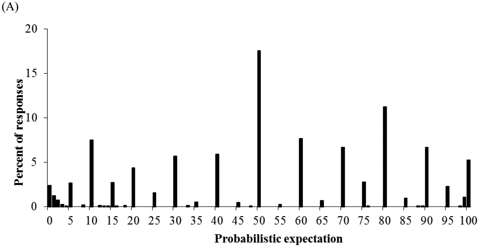
Response distributions of judged probabilities that it will “be very cloudy in your town tomorrow” as provided with (A) open-ended response mode, (B) visual linear scale, and (C) visual magnifier scale (after rounding to the nearest whole number). Black bars reflect use of integers, while white bars reflect use of decimals.

Table 3 shows that response mode differences also held in a multinomial regression controlling respondents’ demographic information, their experiences with the diseases referred to in the probability question, and their explanations given for probability responses (i.e., “no one can know the chances”), as well as other survey conditions, as well as dummy variables for each question (not shown). Standard errors were clustered at the level of the respondent to account for their responses being interrelated. We used Stata’s mfx command so that coefficients could be interpreted as marginal effects, with, for example, a dummy variable with a coefficient of .05 implying that the associated outcome is 5 percentage points more likely when the dummy variable is 1 than when it is zero. Thus, Table 3 shows that, even after controlling for respondent characteristics and other variables, both the visual linear scale and the visual magnifier scale decreased the use of focal responses by respectively 10 and 12 percentage points in the analysis of raw responses, and by respectively 7 and 17 percentage points in the analysis of responses rounded to the nearest integer.

Table 3:

Multinomial regression predicting the use of focal responses (50%, 0%, and 100%) and other responses.

	Raw responses					Responses rounded to nearest integer
Predictor	50%	0%	100%	Other		50%	0%	100%	Other
Response modes
Visual linear scale vs. open-ended	−.04***	−.05***	−.01***	.10***		−.02***	−.04***	−.01***	.07***
Magnifier scale vs. open-ended	−.07***	−.04***	−.01***	.12***		−.10***	−.06***	−.01***	.17***
Respondent characteristics
High numeracy	−.01**	−.01***	.00	.01***		−.01**	−.01***	.00	.02***
College education	−.01***	.00	.00	.01***		−.02***	.00	.00	.02***
Log of income	.00	.00	.00	.00		.00	.00	.00	.00
Age	>.00***	<.00***	<.00*	.00*		>.00***	<.00***	<.00**	>.00*
Gender (female)	.00	.00	<.00***	.00		.00	−.01*	−.00***	.01
Had diseasea	.01***	<.00*	<.00***	−.01*		.01**	<.00*	<.00***	−.01*
Explanations
No one can know the chances (if follow-up)	.02***	.02***	.00	−.03***		.03***	.02***	.00	−.04***
Other survey conditions
Follow-up condition asking for explanations	.00	.00	.00	.00		.00	.00	.00	.00
Question with follow-up asking for explanations	−.01*	.01**	.00	.00		−.01***	.01**	.00	.00
Dying Condition	−.01***	<.00**	<.00***	.01***		−.01***	<.00*	<.00***	.02***
Numeracy first Condition	.00	.00	.00	.00		<.00*	.00	.00	.00
Condition with questions about getting sick given prevention first	.00	.00	.00	.00		.00	.00	.00	.00

^aRefers to the disease that was mentioned in the question.

^***p<.001

^**p<.01,

^*p<.05

Note to Table 3: Dummy variables for individual questions are not shown. Standard errors varied between .01 and .001. Model statistics: pseudo-R²=.23, Wald χ2(90)=7153.53 (for raw responses), p<.0001; pseudo-R²=.19 Wald χ2(90)=7196.23 (for responses rounded to the nearest integer), p<.0001.

3.1.2. The role of numeracy.

Across questions and response modes, respondents with scores below (vs. above) the median of the numeracy scale used more focal responses. In raw responses, 3% more of low-numerate (vs. high-numerate) participants used the three focal responses (95% CI=.02, .04; M=.15, SD=.22 vs. M=.12, SD=.18), t(5290)=5.60, effect size d=.15, p<.001, showing an increase of 2 percentage points for 50% responses (95% CI=.02, .03; M=.06, SD=.13 vs. M=.04, SD=.10), t(5290)=6.73, effect size d=.17, p<.001, an increase of 1 percentage point for 0% responses (95% CI=.01, .02; M=.06, SD=.13 vs. M=.05, SD=.11), t(5290)=3.56, effect size d=.08, p<.01, and no change for 100% responses (95% CI=−.01, .00; M=.03, SD=.06, M=.03, SD=.06), t(5290)=−1.54, effect size d=.00, p=.12. In responses rounded to the nearest integer, 4% more of low-numerate (vs. high-numerate) participants used the three focal responses (95% CI=.03, .05; M=.24, SD=.23 vs. M=.20, SD=.20), t(5290)=6.44, effect size d=.19, p<.001, showing an increase of 4 percentage points for 50% responses (95% CI=.03, .05; M=.11, SD=.16 vs. M=.07, SD=.13), t(5290)=9.08, effect size d=.27, p<.001, no change for 0% responses (95% CI=.00, .01; M=.09, SD=.16 vs. M=.09, SD=.14), t(5290)=1.55, effect size d=.00, p=.12, and a decrease of 1 percentage point for 100% responses (95% CI=−.01, .00; M=.03, SD=.07, M=.04, SD=.07), t(5290)=−2.43, effect size d=.14, p<.05.

As seen in Figure 3, among both low-numerate and high-numerate respondents, each type of focal probability responses was used less often with either alternative visual scale than with the open-ended response mode. This pattern held in raw responses and in responses rounded to the nearest integer (Figure 3). Additionally, t-tests confirmed that these differences were significant for each type of focal response, except for 100% responses (see Table S2).

Figure 3 also allows for numeracy group comparisons by response mode. In the open-ended response mode, low-numerate (vs. high-numerate) respondents used more of the three focal responses, as seen in an increase of 9% in the raw responses, (95% CI=.07, .11) t(1769)=7.51, effect size d=.33, p<.001, and an increase of 8% in the responses rounded to the nearest integer, (95% CI=.06, .10), t(1769)=6.82, effect size d=.33, p<.001. In contrast, the visual linear scale yielded more similar overall focal response use for low-numerate and high-numerate respondents, as seen in raw responses, (95% CI=−.01, .01), t(1762)=.19, effect size d=.00, p=.85, and responses rounded to the nearest integer, (95% CI=.00, .03), t(1762)=2.25, effect size d=.12, p=.03. The visual magnifier scale also showed similar overall focal response use in both numeracy groups, as seen in raw responses, (95% CI=−.01, .01), t(1755)=−.38, effect size d=.00, p=.71, and responses rounded to the nearest integer, (95% CI=−.01, .03), t(1755)=1.38, effect size d=.00, p=.17. Figure 3 shows that this pattern was replicated for the use of 50%, 0%, and 100% responses, such that low-numerate respondents produced especially more of each focal response in the open-ended response mode than in either alternative visual scale (see Table S1 for statistical tests).

Importantly, the multinomial regression analysis confirmed that lower numeracy was related to greater overall use of focal probability responses, especially 50% and 0% (Table 3).¹ Moreover, it showed that there was a significant interaction of response modes with numeracy on the use of different categories of focal responses (Table 4). Thus, although effect sizes varied, both alternative visual scales helped especially low-numerate respondents to somewhat reduce their overall use of focal probability responses.

3.2. Validity of probability responses.

3.2.1. Effects of response modes.

We examined the validity of the probability responses reported with each response mode, in terms of their correlations with self-reports of related beliefs and experiences. To validate judged probabilities of dying, we used respondents’ concurrent reports of their age (M=47.5, SD=15.5), whether they had a serious health problem such as heart disease, diabetes, or high cholesterol (yes=24.1%), and their number of specialist visits in the past year (M=1.39, SD=3.45), which was log transformed due to its long tail (range=0–85). To validate judged probabilities of getting the flu with or without a flu shot, we used respondents’ concurrent reports of whether they had received a flu shot in the past twelve months (yes=22.5%), the likelihood that they would get a flu shot during the next winter (“large” or “very large”=23.2%), and their later reports of whether or not they received a flu shot in the four months after our survey (yes=28.8%). To validate judged probabilities of heart disease with or without aspirin therapy, we used respondents’ concurrent reports of whether they had been taking a low dose of aspirin daily or every other day to prevent heart disease (yes=5.6%), and their likelihood of doing so in the next 5 years (“large” or “very large”=6.2%).

Table 5 shows correlations of judged probabilities of dying in the next 10 years and in the next 20 years with age, log-transformed number of specialist visits, and whether or not respondents reported having a serious health problem. Table 6 shows partial correlations of judged probabilities of getting the flu conditional on getting the flu shot or not, and of judged probabilities of getting heart disease conditional on taking low-dose aspirin or not, with concurrent reports of having engaged in these prevention strategies and concurrent intentions to implement them in the future. For flu shots, we also computed partial correlations of these judged probabilities with later reports of having gotten a flu shot in the four months after the initial survey. We used z-tests comparing Fisher z-transformed correlations to determine whether corresponding correlations were significantly different for the different response modes. Tables 5 and 6 show that each response mode yielded judged probabilities that were significantly correlated to the validation measures, highlighting the validity of probability responses. Most correlations were not significantly different between response modes, indicating roughly equivalent validity of probability responses reported with the open-ended response mode, the visual linear scale, and the visual magnifier scale. However, where significant differences emerged, correlations were somewhat higher when probabilities were reported with the visual linear scale and the visual magnifier scale than with the open-ended response mode. In the one instance that showed a significant difference between the visual linear scale and the visual magnifier scale, the correlation was higher with the visual linear scale (Table 6). Hence, the increased precision encouraged by those response modes did not tend to add noise, and may even have allowed respondents to improve their expression of their probability judgments.

As noted (see 2.2.2), the reported correlations in Tables 5 and 6 were unaffected by whether we used raw probability responses or those rounded to the nearest integer. This was due to the correlation between raw responses and responses rounded to the nearest integer being r=1.00, p<.001, for dying in the next 10 years and in the next 20 years, for getting the flu after getting or not getting a flu shot, and for heart disease with or without aspirin therapy.

3.2.2. The role of numeracy.

We found evidence for response validity among both low-numeracy and high-numeracy respondents, as seen in significant correlations between probability judgments and events (Tables S3 and S4). When significant differences did emerge between numeracy groups, validity was not consistently better for the high-numerate or the low-numerate respondents. Where response mode effects emerged in either numeracy group, correlations were larger with the visual linear scale and the visual magnifier scale than with the open-ended response mode, and the visual magnifier scale performed better than the visual linear scale. As in 3.2.1, these analyses produced the same findings for raw responses and for responses rounded to the nearest integer, due to their correlation of r=1.00, p<.001 for each question (see 2.2.2).

3.3. Respondents’ evaluations of the survey.

3.3.1. Effects of response modes.

An Analysis of Variance (ANOVA) examining the effect of response mode (open-ended, visual linear scale, or visual magnifier scale) and numeracy (high or low) showed a significant yet small effect of response modes on respondents’ evaluations of the survey, F(2, 5236)=4.69, effect size η² =.002, p<.01. The highest evaluations were given to surveys including the visual linear scale: Separate t-tests showed that respondents who received the visual linear scale gave the survey significantly higher evaluations than did those who received the visual magnifier scale (M=3.42, SD=.72 vs. M=3.35, SD=.70; t(3490)=−3.12, effect size d=.10, p<.01), although their evaluations showed no significant differences from those given by respondents in the open-ended response mode (M=3.42, SD=.72 vs. M=3.38, SD=.71; t(3498)=−1.76, effect size d=.06, p=.08). There was no significant difference between the evaluations provided by respondents in the visual magnifier and open-ended conditions (M=3.35, SD=.70 vs. M=3.38, SD=.71; t(3490)=1.35, effect size d=.04, p=.18).

3.3.2. The role of numeracy.

The ANOVA also showed a main effect of numeracy, F(1, 5236)=20.04, effect size η² =.004, p<.001, with high-numerate respondents generally rating the survey as better than low-numerate respondents (M=3.43, SD=.66 vs. M=3.34, SD=.74). However, there was no significant interaction between response mode and numeracy, F(1, 5236)=1.39, effect size η² =.001, p=.25), indicating that the preferences for response modes reported above were similar among high-numerate and low-numerate respondents.

4. DISCUSSION

Assessing the likelihood of future events is an essential component of risk analysis, decision making, and risk communication. Public perception surveys commonly use open-ended questions to assess people’s probabilistic beliefs and perceptions of risk. However, responses tend to show excessive use of 50% due to feelings of uncertainty (Bruine de Bruin & Carman, 2012; Fischhoff & Bruine de Bruin, 1999). Here, we examined whether alternative response modes could reduce the use of 50%, as well as 0% and 100%, which tend to be focal to respondents and raise concerns about response inaccuracies (Hurd, 2009). Respondents assessed the probability of dying, getting the flu, and experiencing other health-related events. They were randomly assigned to an open-ended response mode that asked them to generate their own response between 0% and 100%, a visual linear scale ranging from 0% to 100%, or a visual magnifier scale allowing for even more precision. The results reported here showed that, compared to an open-ended response mode, both visual scales reduced the use of focal responses (50%, 0%, and 100%), showing medium to large effect sizes. In raw responses, the use of focal responses was reduced by 26 percentage points with either scale as compared to the open-ended response mode. In responses recorded as the nearest integer, focal responses were reduced by 17 percentage points with the linear scale and 11 percentage points with the magnifier scale, as compared to the open-ended response mode. Visual scales reduced the use of focal responses especially among low-numerate individuals.

Moreover, the reduced use of these three focal responses did not harm the response validity of either visual scale, as compared to the open-ended response mode. Validity was similar across response modes, suggesting that the visual scales did not add noise to the assessment of subjective probabilities as compared to the open-ended response mode. In some instances, responses given on the visual scales even showed slightly improved validity, as compared to open-ended responses. Valid responses were provided with each of the three response modes. For example, judged probabilities of dying were significantly related to age, judged probabilities of getting the flu if not getting a flu shot were significantly related to getting a flu shot in the four months after our survey, and judged probabilities of getting heart disease if not taking aspirin were significantly related to intentions to take aspirin.

Respondents tended to evaluate the survey as most positive when it presented the visual linear scale, independent of their numeracy skills. Although effect sizes were small, this finding suggests that the visual linear scale did not increase respondent burden as compared to the traditional open-ended response mode. Based on these findings, we recommend that probability elicitation efforts and consumer surveys replace their open-ended response modes with a visual linear scale rather than with a visual magnifier scale.

Like any study, ours has limitations. One limitation of the presented work is that response mode effects were examined in web-based surveys only. In our previous research, we have conducted paper-based surveys, in-person interviews, and even telephone interviews in which we provided respondents with a visual response mode. If our present findings generalize to those survey modes, then visual response modes should reduce the use of focal responses and improve the validity of reported responses. A second limitation is that both visual scales recorded responses with two decimals, perhaps artificially introducing precision and reducing the use of focal responses of 50%, 0%, and 100%. That issue may have especially affected the visual magnifier scale, because it only enlarged only a limited area (between −0.50% and +0.50%) around the initial click. In contrast, hardly any open-ended responses were entered with decimals. However, we found that focal responses were less likely to be used with visual scales independent of whether responses were analyzed as initially entered into the response mode or after rounding to the nearest integer.

One question that arises when examining the seemingly excessive use of 50%, 0% and 100% responses, is how many of these responses would be appropriate. It has been suggested that the proportion of appropriate (vs. inappropriate) focal responses can be assessed in comparison to the rest of the response distribution (Bruine de Bruin et al., 2002). For example, the inappropriate use of 50% is seen in the extent to which the relative use of that response exceeds the amount that would fit with overall shape of the rest of the response distribution (Bruine de Bruin et al., 2002). Visual inspection of response distributions (e.g., Figure 2) confirms previous findings that visual linear scales and visual magnifier scales reduce the relative overuse of 50% response as compared to other probability responses.

Here, we examined only the usefulness of response modes for assessing numerical subjective probabilities. Others have found that responses to verbal probability scales predict behaviors and outcomes as well as responses to numerical probability scales (Weinstein & Diefenbach, 1997; Windschitl & Wells, 1996), even when using visual linear scales similar to those presented here (Woloshin et al., 2000). Although verbal probability scales may be especially helpful with contexts and samples that are characterized by less deliberate numerical thinking (Windschitl et al., 1996), they do not allow direct comparisons of respondents’ probability judgments (e.g., of surviving until a certain age) and actual risk statistics (e.g., from statistical life tables) so as to assess levels of under- or overestimation. Hence, the choice to use verbal probability scales or numerical ones should depend on researchers’ goals.

In conclusion, our results suggest that presenting a visual linear scale or a visual magnifier scale instead of an open-ended response mode allows respondents to express their subjective numerical probabilities with more precision, without harming response validity or respondents’ evaluation of the survey. Improved measurement of people’s probability judgments should benefit probability elicitation efforts relevant to risk analysis, decision making, and risk communication.