Epidemic model on a network: Analysis and applications to COVID-19

Abstract

We analyze an epidemic model on a network consisting of susceptible–infected–recovered equations at the nodes coupled by diffusion using a graph Laplacian. We introduce an epidemic criterion and examine different isolation strategies: we prove that it is most effective to isolate a node of highest degree. The model is also useful to evaluate deconfinement scenarios and prevent a so-called second wave. The model has few parameters enabling fitting to the data and the essential ingredient of importation of infected; these features are particularly important for the current COVID-19 epidemic.

Highlights

• •Mathematical analysis of a simple epidemic model on a network.
• •We introduced an epidemic criterion and examined different isolation strategies.
• •We evaluated deconfinement scenarios to prevent a second wave.

1. Introduction

Many models of the propagation of an epidemic such as the current COVID-19 [1] involve a network. This can be a contact network between individuals. Then, the network is oriented and is used to understand how a given individual can infect others at the very early stages. The models are typically probabilistic, see [2] for example. Once the epidemic is established, the geographical network becomes important. There, nodes represent locations and edges the means of communication; for COVID-19 these are the airline routes [3]. Such a network is non oriented and the important nodes are the ones that are most connected.

One of simplest models of a disease is the Kermack–McKendrick system of equations [4] involving three populations of susceptible, infected and recovered individuals $(S,I,R)$. Using this model together with a probability transition matrix [5] for the geographic coupling, Brockman and Helbling [6] performed a remarkable study of the propagation of well-known epidemics like SARS or H1N1 due to airline travel. They emphasized that the fluxes between the nodes govern the propagation of the epidemic.

In this article, we consider $(S,I,R)$ Kermack–McKendrick equations coupled to a network through a graph Laplacian matrix [7]. The combination of the simple SIR dynamics with the diffusion yields the essential ingredients to model and understand an epidemic, such as the COVID-19. In particular,

• •there are few parameters so that fitting to data can be successful,
• •it contains the essential ingredient of importation of infected subjects from country to country.

The epidemic front is controlled by the availability of susceptibles. If susceptibles are large enough, the front cannot be stopped. The number of susceptibles varies from node to node. Reducing this number at a given location can be done through isolation. This is expensive and cannot be done for the whole network. It is therefore important to address the question: what nodes are more useful to isolate to mitigate the epidemic?

Using this model together with the detailed data available [8], [9], we predicted the onset of the COVID-19 epidemic in Mexico [3]. The present article is devoted to the detailed analysis of the model. We first prove that it is well-posed and that solutions remain positive. We introduce an epidemic criterion that generalizes the well-known $R_0$ of the scalar case. For small diffusion, nodes are almost decoupled and an outbreak occurs at a node if the local $R_0$ is larger than one. When the diffusion is moderate, the epidemic criterion depends on the network and when there is an outbreak, it starts synchronously on the network. Using this criterion, we define an isolation policy. We find that it is most useful to isolate the high connectivity nodes and not efficient to isolate neighbors. For the particular case of the COVID-19 we discuss the effect of deconfining; the model shows that allowing circulation between heavily and weakly infected areas will prolong the outbreak in the latter.

The article is organized as follows. In Section 2, we introduce the model, discuss its main features and present the epidemic criterion. Section 3 shows a simple six node network based on the country of Mexico; there the effect of isolation is discussed. The COVID-19 disease is studied in Section 4 and we show the estimation of the time of outbreak in Mexico. The important issue of deconfinement is studied in Section 5. We conclude in Section 6.

2. The model and epidemic criterion

One of the main models to describe the time evolution of the outbreak of an epidemic is the Kermack–McKendrick model [4]

$$\left\{\begin{array}{c}\dot{S}=-\beta SI,\hfill \\ \dot{I}=\beta SI-\gamma I\hfill \\ \dot{R}=\gamma I\hfill \end{array}\right)$$ (1)

where the dynamics of transmission depends of the frequency and intensity of the interactions between (healthy) susceptible $S$ and infected individuals $I$ and produce recovered individuals $R$. The parameters $\beta$ and $\gamma$ are the infection rate and the recovery rate. The model conserves $N=S+I+R$ the total number of individuals. Note that $R$ is essentially the integral of $I$ and therefore plays no role in the dynamics. We will omit it below and only discuss $S$ and $I$.

An epidemic occurs if $\beta S-\gamma >0$ [4]. At $t=0$, $S=1$ so that an infection occurs if the infection factor defined as

$$R_0\equiv \frac{\beta }{\gamma },$$ (2)

is greater than one. An important moment in the time evolution of $S$ and $I$ is when the number of infected is maximum. The corresponding values $(S^{\ast },I^{\ast })$ can be calculated easily; we give the derivation in the Appendix A, Appendix B. The expressions are

$$S^{\ast }=\frac{1}{R_0},$$ (3)

$$I^{\ast }=I_0+S_0-\frac{1}{R_0}(1+log\left(R_0{S}_0\right))$$ (4)

Note that $I^{\ast }$ and $S^{\ast }$ depend strongly on $R_0$. Take for example $\gamma =0.625$ and different values of $\beta$.

$\beta$	$R_0$	$S^{\ast }$	$I^{\ast }$
2.5	4	0.25	0.403
1.5	2.4	0.417	0.218
1.1	1.76	0.568	0.111

The value of $I^{\ast }$ depends also on the initial number of susceptibles $S_0$ which is smaller than the total number $N$. Generally, a large $N$ gives a large $S_0$ and $I^{\ast }$.

2.1. SIR on a network

We consider a geographic network of cities connected by roads or airline routes. This introduces a spatial component so that $(S,I)$ become vectors; we also drop $R$. This is similar to Murray’s model where he introduces spatial dispersion in an SI model using a continuous Laplacian term [10]. The evolution at a node $j$ in a network of $n$ nodes reads

$${\dot{S}}_j=-\beta \frac{S_j}{N_j}{I}_j+ϵ\sum _{k\sim j}(S_k-S_j),$$ (5)

$${\dot{I}}_j=\beta \frac{S_j}{N_j}{I}_j-\gamma I_j+ϵ\sum _{k\sim j}(I_k-I_j),$$ (6)

where $N_j$ is the population at node $j$, the ${\sum }_{k\sim j}$ is the exchange with the neighboring nodes $k$ of $j$ and where $ϵ$ is a constant. The main difference with the model of [6] is that we assume symmetry in the exchanges.

The Eqs. (5) can be written concisely as

$$\left\{\begin{array}{c}\dot{S}=ϵ\Delta S-\beta SI,\hfill \\ \dot{I}=ϵ\Delta I+\beta SI-\gamma I.\hfill \end{array}\right)$$ (7)

where $S={(S_1,S_2,\dots ,S_n)}^T,I={(I_1,I_2,\dots ,I_n)}^T,\beta \equiv {(\beta ∕N_1,\beta ∕N_2,\dots ,\beta ∕N_n)}^T$, $\Delta$ is the graph Laplacian matrix [7] and we denote by $SI$ the vector

${(S_1{I}_1,S_2{I}_2,\dots ,S_n{I}_n)}^T$. The infection rate $\beta$ can vary from one geographical site to another while the recovery rate $\gamma$ depends only on the disease. The diffusion $ϵ$ should be small so that the populations involved in that process remain much smaller than the node populations $N_j$. Another point is that the diffusion could act only on the infected population. We chose to put the diffusion on both $S$ and $I$ for symmetry reasons.

The graph Laplacian $\Delta$ is the real symmetric negative semi-definite matrix, defined as

$${\Delta }_{kl}=1\mathrm{if}kl\mathrm{connected},0\mathrm{otherwise};{\Delta }_{kk}=-\sum _{l\ne k}{w}_{kl}.$$ (8)

The graph Laplacian has important properties, see Ref. [7], in particular it is a finite difference approximation of the continuous Laplacian [11]. The eigenvalues of $\Delta$ are the $n$ non positive real numbers ordered and denoted as follows:

$$0=-{\omega }_1^2\ge -{\omega }_2^2\ge \cdots \ge -{\omega }_n^2.$$ (9)

The eigenvectors $\{v^1,\dots ,v^n\}$ satisfy

$$\Delta v^j=-{\omega }_j^2{v}^j.$$ (10)

and can be chosen to be orthonormal with respect to the scalar product in ${\mathbb{R}}^n$, i.e. $v^i\cdot v^j={\delta }_{i,j}$ where ${\delta }_{i,j}$ is the Kronecker symbol.

2.2. Well posedness and positivity

The model (7) is well posed in the sense that the solution remains bounded. We show this in the Appendix A, Appendix B using standard techniques.

The biological domain of the system is

$$\Omega =\{(S,I):S\ge 0;I\ge 0\}.$$

Let us show that $\Omega$ is an invariant set for (7) so that the model makes sense in biology. Consider the different axes $S_j=0$ and $I_j=0,j=1,\dots n$. First assume $I_j=0,j=1,\dots n$, then equation (7) reduces to

$$\dot{S}=ϵ\Delta S$$

which conserves the positivity of $S$. Similarly when $S=0$, we get

$$\dot{I}=ϵ\Delta I-\gamma I$$

and again the positivity of $I$ is preserved.

2.3. Epidemic criterion

Here we extend the 1D epidemic criterion of Kermack–McKendrick [4] to our graph model. Initially, the vector $I$ will follow the second equation of (7)

$$\dot{I}=(ϵ\Delta -\gamma )I+\beta SI.$$ (11)

Eq. (11) describes the onset of the epidemic on the network. It can be written

$$\dot{I}=MI$$

where $M$ is the symmetric matrix

$$M=ϵ\Delta -\gamma {Id}_n+\mathrm{diag}(\beta S_1,\beta S_2,\dots ,\beta S_n).$$ (12)

The eigenvalues of $M{\sigma }_1,\dots ,{\sigma }_n$ are real. If one of them is positive, then the solution $I\left(t\right)$ increases exponentially and the epidemic occurs. We can then write

Epidemic criterion : there is an onset of the epidemic if one eigenvalue ${\sigma }_i$ of $M$ is positive.

Two situations occur, depending whether the diffusion is small or moderate. For small diffusion, the contribution of $\Delta$ to $M$ can be neglected. Then each node will develop independently from the others. We will have outbreaks in some and not in others.

When the diffusion is moderate, the Laplacian contributes to $M$. Since $M$ is symmetric the eigenvalues of $M$ remain in the same order as the ones of $\Delta$. This is the interlacing property [7]. Then ${\sigma }_1$ will tend to 0 for $\gamma ,\beta \to 0$. Note also that since $\Vert S\Vert$ decreases with time, the estimate given by the eigenvalues of $M$ indicates the size of the epidemic i.e. $max\Vert I\Vert$. Then, the eigenvector of $M$ for the eigenvalue ${\sigma }_1$ will be almost constant and the epidemic will start synchronously on the network.

The analysis of the moderate diffusion case can be extended when $\beta$ is constant. Expanding $I$ on an orthonormal basis of eigenvectors ($v^k$) of $\Delta$

$$I=\sum _{k=1}^n{\gamma }_k{v}^k,$$ (13)

we get

$${\dot{\gamma }}_k=(-{\omega }_k^2-\gamma ){\gamma }_k+〈\beta SI|v^k〉.$$ (14)

Assume that the susceptible population is constant on the network. Then $\mathrm{diag}(S_1,S_2,\dots ,S_n)=S{\mathrm{Id}}_n$ so that Eq. (16) reduces to

$${\dot{\gamma }}_k=(-{\omega }_k^2-\gamma +\beta S){\gamma }_k.$$ (15)

The epidemic starts if $-\gamma +\beta S>0$ which is a simple generalization of the criterion in the scalar case.

When the population of susceptibles is inhomogeneous and $\beta$ is homogeneous, Eq. (14) becomes

$${\dot{\gamma }}_k=(-{\omega }_k^2-\gamma ){\gamma }_k+\beta \sum _{l=1}^n{\gamma }_l\left(\sum _{j=1}^n{S}_j{v}_j^l{v}_j^k\right).$$ (16)

Then the eigenvectors and the geometry of the network play a role.

3. A simple example

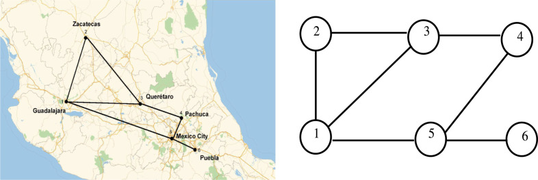
We illustrate the results given above on a 6 node network inspired by the geographical map of Mexico, with six main cities surrounding Mexico city, see Fig. 1. A node represents a city and an edge is a road link between two cities. For simplicity, here we assume that $N_j$ is independent of $j$ so that $I$ and $S$ are given in percentages. This will be the case throughout the article unless specified.

Fig. 1.

Graph of the six main cities in Mexico numbered from 1 to 6: Guadalajara, Zacatecas, Queretaro, Pachuca, Mexico City, Puebla. The links represent the main roads connecting these cities.

The graph Laplacian is

$$\Delta =\left[\begin{array}{cccccc}\hfill -3\hfill & \hfill 1\hfill & \hfill 1\hfill & \hfill 0\hfill & \hfill 1\hfill & \hfill 0\hfill \\ \hfill 1\hfill & \hfill -2\hfill & \hfill 1\hfill & \hfill 0\hfill & \hfill 0\hfill & \hfill 0\hfill \\ \hfill 1\hfill & \hfill 1\hfill & \hfill -3\hfill & \hfill 1\hfill & \hfill 0\hfill & \hfill 0\hfill \\ \hfill 0\hfill & \hfill 0\hfill & \hfill 1\hfill & \hfill -2\hfill & \hfill 1\hfill & \hfill 0\hfill \\ \hfill 1\hfill & \hfill 0\hfill & \hfill 0\hfill & \hfill 1\hfill & \hfill -3\hfill & \hfill 1\hfill \\ \hfill 0\hfill & \hfill 0\hfill & \hfill 0\hfill & \hfill 0\hfill & \hfill 1\hfill & \hfill -1\hfill \end{array}\right].$$

The eigenvalues of this graph Laplacian are

0

−0.721

−1.682

-3.

−3.704

−4.891

The corresponding eigenvectors are

0.4082	−0.2209	−0.2007	−0.5774	0.3084	0.5620
0.4082	−0.4149	−0.5053	0.2887	−0.5670	−0.0323
0.4082	−0.3094	0.0403	0.2887	0.6581	−0.4685
0.4082	−0.0692	0.7590	0.2887	−0.2051	0.3564
0.4082	0.2209	0.2007	−0.5774	−0.3084	−0.5620
0.4082	0.7935	−0.2940	0.2887	0.1140	0.1444

3.1. Influence of the diffusion

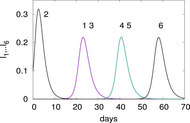
The variable $ϵ$ measures the intensity of the diffusion of $S$ and $I$ on the network. When $ϵ\ll 1$ the diffusion is very weak and the evolution at each node can be decoupled from the one of its neighbors. For larger $ϵ$, the diffusion and reaction occur on similar time periods and need to be analyzed together. To see the influence of the diffusion, we plot in Fig. 2 the evolution of $I_k\left(t\right),k=1,\dots ,6$ for $ϵ=0.1$ (left panel) and $ϵ=10^{-7}$ (right panel).

Fig. 2.

Time evolution $I_k\left(t\right),k=1,\dots ,6$ for an outbreak at node 6 for $ϵ=0.1$ (left panel) and 10⁻⁷ (right panel). The other parameters are $\beta =1.5$ and $\gamma =0.625$.

Note the times of arrival of the infection, first in node 5 the neighbor of node 6, then nodes 1 and 4 and finally nodes 3 and 2. For the large diffusion (left panel of Fig. 2) the peaks are very close and there is a strong influence between the nodes. On the other hand for a small diffusion, the peaks are well separated and the nodes are decoupled. The maximum of $I_k$ is given by the estimate (4).

Infecting node 2 changes the time of arrival of the outbreak as shown in Fig. 3. It reaches first nodes 1 and 3, then nodes 4 and 5 and finally node 6.

Fig. 3.

Time evolution $I_k\left(t\right),k=1,\dots ,6$ for an outbreak at node 2. The parameters are as in Fig. 2 (right panel).

3.2. Isolation policies for large diffusion

We first consider that the diffusion and the nonlinear terms have similar orders of magnitude. We will address the case of weak diffusion in the next section.

When the diffusion is large, one should consider the epidemic on the network as a whole and use the topology of the network to reduce the strength of the outbreak. From the amplitude Eqs. (16), one can devise a strategy of isolation. By this we mean reducing $\beta$ so that the maximal eigenvalue of $M$ is minimum.

We choose

$$ϵ=1,\beta =6.5,\gamma =6.25.$$

Table 1 shows the eigenvalues ${\sigma }_1,\dots ,{\sigma }_n$ of $M$ from (12) when isolating a node of the network, i.e. setting $S_j=0$ at a specific node $j$ and keeping the other nodes the same. We chose $S={(1,1,1,1,1,1)}^T$.

Table 1.

Isolated node $j$ and associated eigenvalues of $M$.

$j$	Degree	${\sigma }_3$	${\sigma }_2$	${\sigma }_1$
6	1	−2.46	−1.30	$1.2210^{-1}$
2	2	−2.14	$-7.8510^{-1}$	$3.8310^{-2}$
4	2	−2.51	$-4.7910^{-1}$	$-1.0610^{-2}$
3	3	−1.44	$-8.2910^{-1}$	$-3.7110^{-2}$
1	3	−1.52	$-6.4110^{-1}$	$-6.7210^{-2}$
5	3	−1.52	$-6.4110^{-1}$	$-6.7210^{-2}$

In the absence of isolation, the largest eigenvalue of the matrix $M$ is $2.510^{-1}$. The table shows that it is most effective to isolate nodes 1,3 and 5. These nodes have the highest degree of the network.

We now isolate two cities in the network. The results are presented in Table 2. We chose

$$ϵ=1,\beta =6.75,\gamma =6.25,$$

and $S={(1,1,1,1,1,1)}^T$.

Table 2.

Isolated nodes $i,j$ and associated eigenvalues of $M$.

$i$	$j$	$d_i$	$d_j$	Neighbors?	${\sigma }_3$	${\sigma }_2$	${\sigma }_1$
5	6	3	1	Yes	−2.97	−1.27	$1.6710^{-1}$
2	3	2	3	Yes	−1.99	$-9.4910^{-1}$	$1.5610^{-1}$
1	2	3	2	Yes	−2.57	$-6.8310^{-1}$	$1.2710^{-1}$
4	6	2	1	No	−3.00	−1.83	$9.1710^{-2}$
1	3	3	3	Yes	−1.31	$-9.6610^{-1}$	$7.5310^{-2}$
3	4	3	2	Yes	−2.26	$-6.2410^{-1}$	$6.0110^{-2}$
2	4	2	2	No	−2.68	$-9.7110^{-1}$	$4.7710^{-2}$
4	5	2	3	Yes	−2.82	$-3.9410^{-1}$	$-9.0810^{-3}$
1	4	3	2	No	−2.61	$-6.1610^{-1}$	$-3.4810^{-2}$
2	6	2	1	No	−2.33	−1.89	$-3.8410^{-2}$
1	6	3	1	No	−2.60	−1.14	$-1.0910^{-1}$
3	6	3	1	No	−2.41	−1.06	$-2.1210^{-1}$
1	5	3	3	Yes	−1.39	$-4.2410^{-1}$	$-2.5010^{-1}$
2	5	2	3	No	−1.89	$-5.4110^{-1}$	$-2.9110^{-1}$
3	5	3	3	No	−1.33	$-5.9710^{-1}$	$-3.3710^{-1}$

Again the high degree nodes 1,3 and 5 are the ones that reduce ${\sigma }_1$ the most and are therefore the most effective when applying isolation. It is also not effective to isolate neighboring nodes.

The results shown in Table 1, Table 2 can be explained in part from the properties of the matrix $M$ and the graph Laplacian $\Delta$. The maximal eigenvalue ${\sigma }_1$ of $M$ verifies [7]

$${\sigma }_1=\underset{\Vert X\Vert =1}{sup}{X}^{T}MX.$$ (17)

We can find inequalities for ${\sigma }_1$ by choosing

$$X={(1,0\dots 0)}^T,X={(0,1,0\dots 0)}^T,\dots$$

Denoting $d_i$ the degree of node $i$, we get

$${\sigma }_1\ge -ϵd_1+\beta S_1-\gamma ,$$ (18)

$${\sigma }_1\ge -ϵd_2+\beta S_2-\gamma ,$$ (19)

$$\dots$$ (20)

$${\sigma }_1\ge -ϵd_n+\beta S_n-\gamma ,$$ (21)

so that

$${\sigma }_1\ge -\underset{k}{min}{d}_k+\beta S-\gamma .$$ (22)

This relation shows that isolating a node that has not smallest degree does not change the estimate. Conversely, if there is a unique node of minimal degree and we isolate it, then the bound changes.

Using similar arguments, it can be shown that isolating two neighboring nodes, say 1 and 2 will be less effective than isolating two non neighboring nodes.

Now we look at what happens if we cut a link, which corresponds to condemning a road for example. Let ${\Delta }^{\prime }$ be the Laplacian of the new graph obtained by deleting a link. Without loss of generality we can assume this link to be between vertices 1 and 2. Then ${\Delta }^{\prime }=\Delta -M$ where

$$M=\left(\begin{array}{ccccc}\hfill -1\hfill & \hfill 1\hfill & \hfill 0\hfill & \hfill \dots \hfill & \hfill 0\hfill \\ \hfill 1\hfill & \hfill -1\hfill & \hfill 0\hfill & \hfill \dots \hfill & \hfill 0\hfill \\ \hfill 0\hfill & \hfill \dots \hfill & \hfill \dots \hfill & \hfill 0\hfill \end{array}\right)$$

$M$ has all eigenvalues equal to $0$ except one which has value $-2$. Applying the Courant–Weyl inequalities, see for example [7], we get the following result for the maximum eigenvalue of ${\Delta }^{\prime }$

$${\sigma }_1^{\prime }\le {\sigma }_1.$$

Note that equality is possible: when $S$ is homogeneous, the maximum eigenvalue of $M$ will always be $-\gamma +\beta S$. In such a case, cutting a link is ineffective.

3.3. Small diffusion and isolation policies

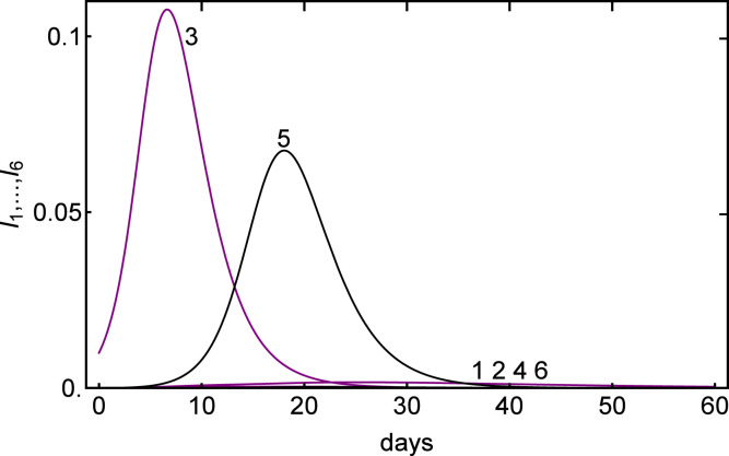
When diffusion is small, the nodes evolve almost independently so that the simple dynamics of the scalar SIR model apply. Then some nodes can be isolated and the epidemic is not seen there. Fig. 4 shows such a situation. We choose

$$\beta =1.98,\gamma =0.5,ϵ=10^{-3}$$

and the initial conditions are given in Table 3 below. The local $R_0$ is also computed and one sees that an outbreak will occur at nodes 1,3 and 5 and not at nodes 2, 4 and 6. Fig. 4 shows the peaks for $I_3$ and $I_5$ and the maxima of $I_3$ and $I_5$ are close to the ones predicted by the SIR formulas (4).

Fig. 4.

Time evolution of the infected for different initial susceptibles at the nodes. The parameters are $\beta =1.98,\gamma =0.5,ϵ=10^{-3}$ and the initial conditions are given in Table 3.

Table 3.

Initial conditions and local $R_0$ for the plots of Fig. 4.

Node $j$	1	2	3	4	5	6
$S_j(t=0)$	0.26	0.14	0.55	0.16	0.5	0.18
$I_j(t=0)$	0	0	0.01	0	0	0
$R_0=\beta \frac{{S_j}_0}{\gamma }$	1.0296	0.5544	2.1780	0.6336	1.9800	0.7128
$I^{\ast }$	0.0001	0.0364	0.1109	0.0227	0.0750	0.0130

4. Propagation of COVID-19

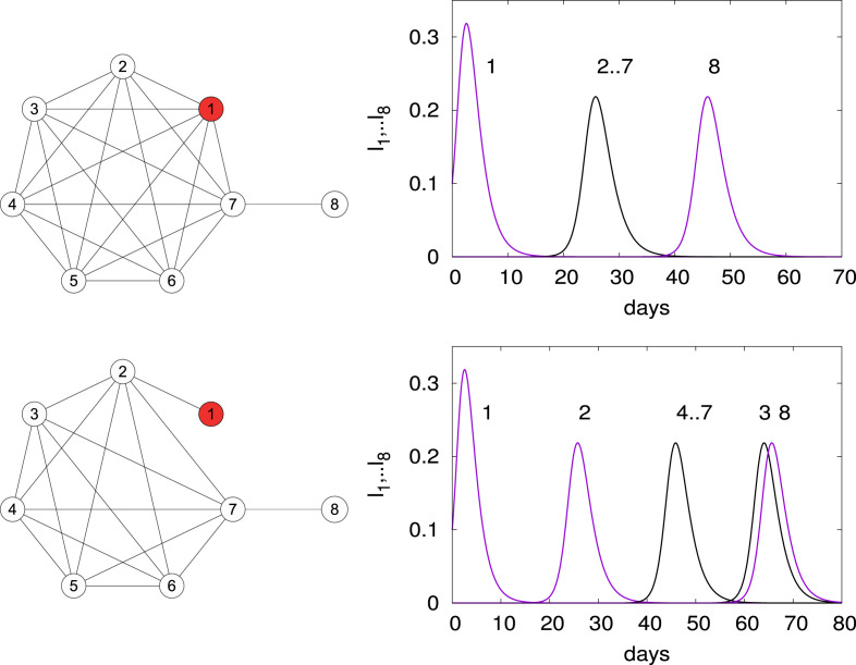
We now consider the propagation of the Corona virus COVID-19 on a network consisting of a complete graph of 7 nodes with an additional link to an 8th node, see top left panel of Fig. 5. The 7 nodes correspond to the following cities or regions, Hubei, Beijing, Shanghai, Japan, western Europe, eastern USA and western USA and the 8th node is Mexico. The links are the main airline routes. We assume a complete graph because airline routes connect any two of these regions.

Fig. 5.

Propagation of the COVID-19: the network composed of seven main regions/cities in the world forming a complete graph is shown in the top left panel and the time evolution of the infected per node is shown in the top right panel. In the bottom panels, node 1 (Hubei) is only connected to node 2 (Beijing) and isolated from the other nodes: see graph in the bottom left panel. The corresponding time evolution of the infected is shown in the bottom right panel. The parameters are $\beta =0.5,\gamma =0.2$ and $ϵ=10^{-6}{\mathrm{days}}^{-2}$. At time $t=0$ we assume $I_1=0.1,I_k=0,k\ne 1$.

The parameters chosen are $\beta =0.5,\gamma =0.2$ and $ϵ=10^{-6}{\mathrm{days}}^{-2}$. These were suggested by very early estimations of the outbreak in Wuhan. Using the data from the John Hopkins website [8] and our model, we estimated the starting time of the outbreak in Mexico to be from March 20 to March 30 2020 [3]. These results were shared with the Ministry of health of Mexico at the end of February 2020 so that preparations could be made. In the present article, we analyze the model; we therefore comment briefly the evolutions obtained in [3] as an interesting case.

The top right panel of Fig. 5 shows the time evolution in days of the infected in the different nodes. The simulation is started at node 1 (Hubei in red in Fig. 5) with $I_1=0.1$ and the other nodes are set at 0. The susceptibles are set to 1 everywhere. As expected the maximum $I_1^{\ast }=0.32$ and the subsequent maxima $I_j^{\ast }=0.21,j=2,\dots 8$. Notice how the nodes 2–7 start simultaneously while node 8 is delayed. Communications with the province of Hubei were restricted at the end of December 2019. To model this, we now consider that node 1 is only connected to node 2 which forms a complete graph with nodes 3–7, see bottom left panel of Fig. 5. The infected are shown in the bottom right panel; as expected the epidemic first arrives in node 2 then synchronously in nodes 3–7 and then in node 8.

To test the effect of having different $\beta$ s at each node we increased ${\beta }_3$, reduced ${\beta }_4$ and kept the other $\beta$ s the same. Then the epidemic arrives sooner at node 3 and later at node 4. As expected from the formulas (4) $I_3^{\ast }>I_j^{\ast }>I_4^{\ast }$ for $j=5,6,7$, see [3].

5. Confinement and deconfinement

Since there is no vaccine for COVID-19 disease and the mortality is relatively high, many countries put in place a confinement or measures to reduce the movement of the population.

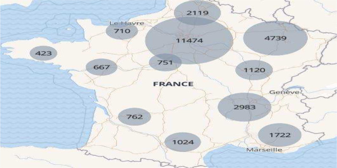
China confined the Hubei region around January 22, Italy confined its population on March 9, France on March 17 and so on. In the middle of the epidemic, Spain and France reached a situation like the one shown in Fig. 6. This picture shows the number of patients in hospitals on April 5 2020 for the 12 different regions of mainland France (see Table 4), the data was obtained from the website [12]. Note how some regions are highly infected while others have many fewer cases. To use this regional data of France, one could establish a graph of the main roads and railways connecting the main cities, very much like the one for Mexico in Fig. 1.

Fig. 6.

Map of the number of patients in hospital due to COVID-19 in France for the twelve different regions of France (see Table 4) on April 5 2020.

Table 4.

The twelve regions of mainland France, the main cities and the number of patients in hospital on April 5 2020.

Region	Main cities	Number of patients
Ile de France	Paris	11474
Grand est	Strasbourg, Mulhouse	4739
Auvergne-Rhone-Alpes	Lyon, Grenoble, Clermont-Ferrand	2983
Provence-Alpes-Cote d’Azur	Marseille, Nice	1722
Hauts de France	Lille, Valenciennes	2119
Bourgogne-Franche Comté	Dijon, Besancon	1120
Occitanie	Toulouse, Montpellier	1024
Nouvelle Acquitaine	Bordeaux	762
Centre Val de Loire	Orleans, Tours	751
Normandie	Rouen, Caen, Le Havre	710
Pays de la Loire	Nantes	667
Bretagne	Rennes, Brest	423

Let us now consider the confinement. It can be implemented by

• (i)reducing the contact ratio ${\beta }_j$ of each node $j$
• (ii)reducing the diffusion $ϵ$, i.e. the travel between nodes

When deconfining the population once the peak of the epidemic has passed the two options (i) and (ii) need to be relaxed, so as to avoid a so-called second wave. This happens in particular when the epidemic affected a small fraction of the total number $N$. Then, relaxing $\beta$ or equivalently increasing $N$ causes a number of new susceptibles to enter the reaction and therefore produce a second peak of infection. The model (5) allows to analyze the effect of the two options. We do this separately but note that in reality both act together and effects can cancel.

Consider option (i). For this, we study the situation at a single node. We choose the parameters

$$\beta =0.33,\gamma =0.13,$$

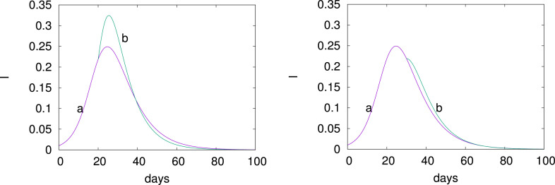
and the computation is started at $t=0$ with $S_0=1,I_0=0.01$. Here, as before, the units of $I$ are percentages. In Fig. 7, we show the evolution of the infected for a sudden increase of $\beta$ from 0.33 to 0.5 at $t=20$ before the peak (left panel, line b) and $t=30$ after the peak (right panel, line b). Clearly, the deconfinement before the peak causes many more infections and could saturate the hospitals. Deconfining after the peak as shown on the right panel of Fig. 7 is harmless. Only one node is involved.

Fig. 7.

Deconfinement (i) by increasing $\beta$ at a single node. Evolution of $I\left(t\right)$ for a sudden increase of $\beta$ from 0.33 (curve a) to 0.5 (curve b) at $t=20$ before the peak (left panel) and $t=30$ after the peak (right panel); $\gamma =0.13$.

Another way of deconfining is to relax option (ii), that is allowing travel from one node to another. This corresponds to increasing the diffusion which can bring infected from large centers to small centers. To illustrate this, consider the graph of two nodes shown in Fig. 8. It corresponds for the example of France Fig. 6, to allowing travel between the large urban area of Paris and the much less populated Normandy. The capacity of node 1 (Paris) is $N_1=2010^6$ while $N_2=10^6$. Now, $I_1$ and $I_2$ are actual numbers and not percentages. We consider Eqs. (5) where $S_j,I_j$ have been normalized by $10^6$. The parameters are

$${\beta }_1=\frac{\beta }{N_1}=0.025,{\beta }_2=\frac{\beta }{N_2}=0.5,\gamma =0.2,ϵ=10^{-6}.$$

The initial conditions are

$$S_1=20,S_2=1,I_1=0.1,I_2=0.01,$$

in millions. To model option (ii) we suddenly increase the diffusion parameter $ϵ$ to $ϵ=10^{-2}$.

Fig. 8.

The two node graph representing the interaction between a large city and a small city.

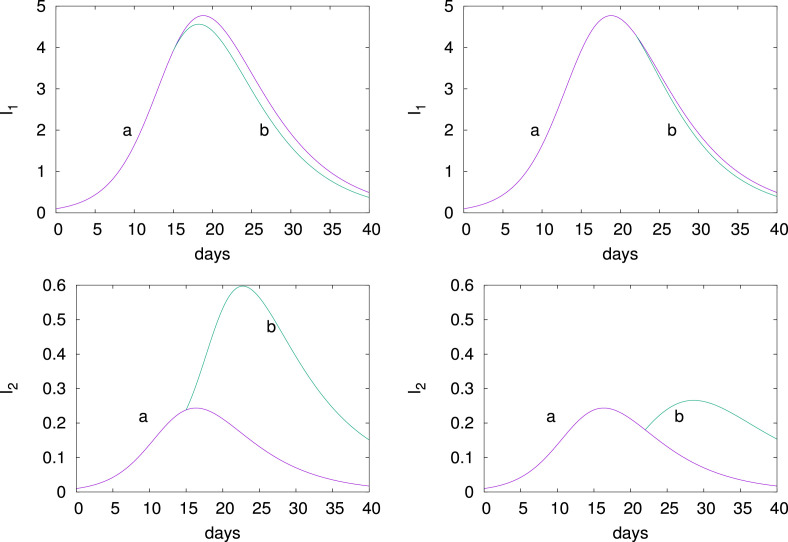
Fig. 9 shows $I_1\left(t\right)$ (top panels) and $I_2\left(t\right)$ (bottom panels) when deconfining before the peak (left panels) and after the peak (right panels). The curves $I_1\left(t\right),I_2\left(t\right)$ before and after deconfining are indicated by $a$ and $b$ respectively. The $y$ scale are in millions. Deconfining before the peak is not so harmful for node 1 while it is catastrophic for node 2, $I_2$ is multiplied by 3. After the peak, a sudden deconfinement prolongs the epidemic at node 2.

Fig. 9.

Deconfinement (ii). Time evolution $I_1\left(t\right),I_2\left(t\right)$ for the two node graph shown in Fig. 8 when $ϵ$ is increased from 10⁻⁶ (curve a) to 10⁻² (curve b), at $t=15$ before the epidemic peak (left panel) and at $t=22$ (right panel) after the epidemic peak. The units are in millions. See text for parameters and initial conditions.

6. Discussion and conclusion

For the COVID-19 epidemic, few articles have addressed the coupling of an epidemic model to the geographical landscape. The subject is difficult as mobility is not well understood at microscopic level. It is also difficult to extract a model from the available data.

In the Ref. [13], the authors estimated how mobility and transmissibility affect the onset of the epidemic in the cities adjacent to Wuhan in the territory of China. They found that reducing the mobility between cities by some factor did not change the time of onset of the epidemic peaks. This is unexpected as seen in the present article where reducing the mobility by orders of magnitude delays the onset of the epidemic. Also the world data [8] and [9] shows clearly the epidemic peaking first in China, then in Iran, Italy and so on. Therefore, the result of [13] might be due to the fact that small changes are effected on the mobility. It might also be due to the model of mobility chosen.

For Brazil, the study [14] considers a six equation compartmental model coupled to a complex mobility scheme. The authors show that the epidemic curves vary “enormously” over different geographic scales. Outbreaks can start in big cities and propagate to the countryside or there might be multiple foci of infection. It is difficult to get a view of the epidemic at the scale of the network with such a complex model.

In our study, we used the simplest susceptible–infected equations at the nodes coupled by a geographic diffusion term. This contains the essential ingredient of importation of infected subjects from country to country. We have kept the number of parameters to a minimum so that fitting the data can be successful. This is particularly important for the present epidemic of COVID-19 where one wants to get a global picture at the level of the network.

The Laplacian models well the symmetric flow from one node to another. This is a first order approximation of the spreading of infected in terms of diffusion. One can refine the approximation using a kernel of an anomalous or stochastic diffusion but then more careful measures of the ways the infection travels are needed.

On the analysis side, using this model, we generalized the well-known epidemic criterion of Kermack–McKendrick. For small diffusion, outbreaks occur at different times as the disease advances through the network. A larger diffusion will cause the outbreak to occur synchronously on the network. Using this criterion, we designed an isolation policy: we find it best to isolate high degree nodes and not efficient to isolate neighbors.

We also discussed the important aspect of deconfining a region after the outbreak. Circulation between highly infected regions and less impacted areas should be reduced to prevent the spread of infected to the latter. Large clusters should be carefully controlled.

Finally the study points out the usefulness of having accurate data at country and local levels (cities, neighborhoods and hospitals).

CRediT authorship contribution statement

F. Bustamante-Castañeda: Software, Validation. J.-G. Caputo: Writing - original draft. G. Cruz-Pacheco: Writing - review & editing. A. Knippel: Conceptualization, Methodology. F. Mouatamide: Software, Validation.

Declaration of Competing Interest

The authors declare that they have no known competing financial interests or personal relationships that could have appeared to influence the work reported in this paper.

Appendix A. Analysis of the SIR model

The expressions (4) may easily obtained in terms of $R_0$ as it is shown below.

From $\dot{I}=0$ we obtain

$$S^{\ast }=\frac{\gamma }{\beta }=\frac{1}{R_0}.$$ (23)

Dividing the second equation of (1) by the first, we get

$$\frac{dI}{dS}=-1+\frac{\gamma }{\beta S},$$

which can be integrated to yield

$$I=I_0+S_0-S+\frac{\gamma }{\beta }log\frac{S}{S_0},$$ (24)

where we assumed $S(t=0)=S_0$ and $I(t=0)=I_0$. Then one can compute $I^{\ast }$

$$I^{\ast }=I_0+S_0-S^{\ast }+\frac{\gamma }{\beta }log\frac{S^{\ast }}{S_0}.$$ (25)

Assuming $S_0=1$, Eqs. (23), (25) can written in terms of $R_0$ as

$$S^{\ast }=\frac{1}{R_0},I^{\ast }=I_0+S_0-\frac{1}{R_0}(1+log\left(R_0{S}_0\right))$$ (26)

The time $t^{\ast }$ corresponding to $S^{\ast },I^{\ast }$ can be calculated in the following way.

From the second equation of (1) one can write

$$\frac{dt}{dS}=-\frac{1}{\beta }\frac{1}{SI}=-\frac{1}{\beta }\frac{1}{S(I_0+S_0-S+\frac{1}{R_0}logS)},$$

where we have substituted $I\left(S\right)$ from (24). Integrating this expression from $S^{\ast }$ to $S_0$ yields the value $t^{\ast }$

$$t^{\ast }=\frac{1}{\beta }{\int }_{S^{\ast }}^{S_0}\frac{dS}{S(I_0+S_0-S+\frac{1}{R_0}logS)}.$$ (27)

This expression can be used to predict the time $t^{\ast }$ from data.

Appendix B. Well-posedness of the model

To prove the well-posedness, we rewrite the system (7) as the following abstract differential equation:

$$\left\{\begin{array}{c}{x}^{\prime }\left(t\right)=Ax\left(t\right)+f\left(x\left(t\right)\right)\hfill \\ x\left(0\right)=x_0\in R^n\hfill \end{array}\right)$$ (28)

where $x≔\left(\begin{array}{c}\hfill s\hfill \\ \hfill i\hfill \end{array}\right)$, $A$ is the matrix given by

$$A≔\left(\begin{array}{cc}\hfill \Delta \hfill & \hfill 0\hfill \\ \hfill 0\hfill & \hfill \Delta \hfill \end{array}\right)$$

and $f:R^n\times R^n⟶R^{2n}$ defined by

$$f\left(x\right)≔\left(\begin{array}{c}\hfill -\beta si\hfill \\ \hfill \beta si-\gamma i\hfill \end{array}\right)$$

and $x_0≔\left(\begin{array}{c}\hfill S_0\hfill \\ \hfill I_0\hfill \end{array}\right)$.

It is clear that, the function $f$ is $L_f$-Lipschitzian with $L_f$ depends only on $\beta$ and $\gamma$. Now, we formulate the well-posedness theorem, which is the main theorem of this section:

Theorem B.1

Given $x_0\in R^n$ . Then, Eq. (28) has a unique solution satisfying the following formula:

$$x\left(t\right)=e^{tA}{x}_0+{\int }_0^t{e}^{(t-s)A}f\left(x\left(s\right)\right)ds,t\ge 0.$$ (29)

Proof

Let $x_0\in R^n$ and $T>0$. Consider the mapping $\Gamma :C⟶C$ given by

$$\Gamma u\left(t\right)=e^{tA}{x}_0+{\int }_0^t{e}^{(t-s)A}f\left(u\left(s\right)\right)ds$$

where $C≔C([0,T],R^n)$. Let us prove that $\Gamma$ is a contraction. Indeed, let $u,v\in C$, then

$$\Vert \Gamma \left(u\left(t\right)\right)-\Gamma \left(v\left(t\right)\right)\Vert \le {\int }_0^t{e}^{(t-s)\Vert A\Vert }\Vert f\left(u\left(s\right)\right)-f\left(v\left(s\right)\right)\Vert ds\le L_f{\int }_0^t{e}^{(t-s)\Vert A\Vert }\Vert u\left(s\right)-v\left(s\right)\Vert ds\le L_f{e}^{T\Vert A\Vert }{\int }_0^t\Vert u\left(s\right)-v\left(s\right)\Vert ds\le L_f{e}^{T\Vert A\Vert }t{\Vert u-v\Vert }_{\infty }.$$

On the other hand

$$\Vert {\Gamma }^2\left(u\left(t\right)\right)-{\Gamma }^2\left(v\left(t\right)\right)\Vert =\Vert \Gamma \left(\Gamma u\left(t\right)\right)-\Gamma \left(\Gamma v\left(t\right)\right)\Vert \le L_f{e}^{T\Vert A\Vert }{\int }_0^{t}s\Vert \Gamma \left(u\left(s\right)\right)-\Gamma \left(v\left(s\right)\right)\Vert ds\le \frac{{\left(L_f{e}^{T\Vert A\Vert }t\right)}^2}{2}{\Vert u-v\Vert }_{\infty }.$$

Hence, by iterating for $n\ge 1$, we conclude that

$$\Vert {\Gamma }^n\left(u\left(t\right)\right)-{\Gamma }^n\left(v\left(t\right)\right)\Vert \le \frac{{\left(L_f{e}^{T\Vert A\Vert }T\right)}^n}{n!}{\Vert u-v\Vert }_{\infty }.$$

Now, for $n$ large enough,

$$\frac{{\left(L_f{e}^{T\Vert A\Vert }T\right)}^n}{n!}<1.$$

The mapping ${\Gamma }^n$ is a contraction. Therefore, by using the iterating fixed point theorem $\Gamma$ is also a contraction. Consequently, the system (13) has a unique solution which is given by (14).  □

References

- 1.World Health Organization, Novel Coronavirus (2019-nCoV). Situation report [cited 2020 March 06 2020], https://www.who.int/docs/default-source/coronaviruse/situation-reports/20200121-sitrep-1-2019-ncov.pdf?sfvrsn=20a99c10_4.
- 2.Wilkinson R.R., Sharkey K.J., Ball F.G. The relationships between message passing, pairwise, Kermack–McKendrick and stochastic SIR epidemic models. J. Math. Biol. 2017;75:1563–1590. doi: 10.1007/s00285-017-1123-8. [DOI] [PMC free article] [PubMed] [Google Scholar]
- 3.Cruz-Pacheco G., Bustamante-Castañeda J.F., Caputo J.-G., Jiménez-Corona M.-E., Ponce-de León-Rosales S. Dispersion of a new coronavirus SARS-CoV-2 by airlines in 2020: Temporal estimates of the outbreak in Mexico. Clin. Transl. Invest. 2020;72(3):138–143. doi: 10.24875/RIC.20000113. http://clinicalandtranslationalinvestigation.com/frame_esp.php?id=267 [DOI] [PubMed] [Google Scholar]
- 4.Kermack W.O., McKendrick A.G. A contribution to the mathematical theory of epidemics. Proc. R. Soc. Lond. 1927;115:700–721. [Google Scholar]
- 5.Asmussen S. Applied Probability and Queues. Springer; 2003. (Stochastic Modelling and Applied Probability). [Google Scholar]
- 6.Brockmann D., Helbling D. The Hidden geometry of complex, Network-driven contagion Phenomena. Science. 2013;13 doi: 10.1126/science.1245200. [DOI] [PubMed] [Google Scholar]
- 7.Cvetkovic D., Rowlinson P., Simic S. An Introduction to the Theory of Graph Spectra. no. 75. 2001. (London Mathematical Society Student Texts). [Google Scholar]
- 8.Coronavirus COVID-19 global cases by Johns Hopkins CSSE, https://github.com/CSSEGISandData/COVID-19/blob/master/csse_covid_19_data/csse_covid_19_time_series/time_series_19-covid-Confirmed.csv.
- 9.https://www.worldometers.info/coronavirus/#countries.
- 10.Murray J.D. Springer Berlin; 2003. Mathematical Biology, Vol. 2. [Google Scholar]
- 11.Dahlquist G., Bjorck A., Anderson N. Prentice Hall; 1974. Numerical Methods. [Google Scholar]
- 12.https://veille-coronavirus.fr/.
- 13.Wu J.T., Leung K., Leung G.M. Nowcasting and forecasting the potential domestic and international spread of the 2019-nCoV outbreak originating in Wuhan, China: a modelling study. Lancet. 2019;395:689–697. doi: 10.1016/S0140-6736(20)30260-9. [DOI] [PMC free article] [PubMed] [Google Scholar]
- 14.G.S. Costa, W. Cota, S.C. Ferreira, Metapopulation modeling of COVID-19 advancing into the countryside: an analysis of mitigation strategies for Brazil, 10.1101/2020.05.06.20093492. [DOI]