3D-MICE: integration of cross-sectional and longitudinal imputation for multi-analyte longitudinal clinical data

Abstract

Objective

A key challenge in clinical data mining is that most clinical datasets contain missing data. Since many commonly used machine learning algorithms require complete datasets (no missing data), clinical analytic approaches often entail an imputation procedure to “fill in” missing data. However, although most clinical datasets contain a temporal component, most commonly used imputation methods do not adequately accommodate longitudinal time-based data. We sought to develop a new imputation algorithm, 3-dimensional multiple imputation with chained equations (3D-MICE), that can perform accurate imputation of missing clinical time series data.

Methods

We extracted clinical laboratory test results for 13 commonly measured analytes (clinical laboratory tests). We imputed missing test results for the 13 analytes using 3 imputation methods: multiple imputation with chained equations (MICE), Gaussian process (GP), and 3D-MICE. 3D-MICE utilizes both MICE and GP imputation to integrate cross-sectional and longitudinal information. To evaluate imputation method performance, we randomly masked selected test results and imputed these masked results alongside results missing from our original data. We compared predicted results to measured results for masked data points.

Results

3D-MICE performed significantly better than MICE and GP-based imputation in a composite of all 13 analytes, predicting missing results with a normalized root-mean-square error of 0.342, compared to 0.373 for MICE alone and 0.358 for GP alone.

Conclusions

3D-MICE offers a novel and practical approach to imputing clinical laboratory time series data. 3D-MICE may provide an additional tool for use as a foundation in clinical predictive analytics and intelligent clinical decision support.

INTRODUCTION

Researchers are increasingly working to “mine” clinical patient data to derive new clinical knowledge,¹ with a goal of enabling greater diagnostic precision, better personalized therapeutic regimens, improved clinical outcomes, and more efficient utilization of health care resources.² However, clinical data quality is often one of the major impediments to deriving optimal knowledge from clinical data.² Unlike experimental data that are collected per a research protocol, the primary role of clinical data is to help clinicians care for patients, so the procedures for their collection are not often systematic. Clinically appropriate data collection often does not occur on a regular schedule, but rather is guided by patient conditions and clinical or administrative requirements. Thus, electronic health record (EHR) data are often available only at irregular intervals that vary among patients and types of data. In turn, even with complete EHR data, most aspects of patients’ clinical states will be unmeasured, unrecorded, and unknown for most patients at most time points. While this “missing data” may be fully clinically appropriate, machine learning algorithms cannot directly accommodate missing data.³ Accordingly, missing data can hinder EHR knowledge discovery and data-mining efforts.

One approach to addressing missing data is simply to exclude incomplete cases. However, excluding patients or cases with incomplete data from analyses can introduce bias⁴ and limit the generalizability of findings. Moreover, in many real-world settings, most if not all patients have some missing data, and thus excluding patients with missing data may leave few if any patients for analysis.

Rather than excluding cases with missing data, a better strategy usually involves applying various statistical “imputation” techniques to raw datasets to “fill in” missing data elements. Imputation uses available data and relationships they contain to predict point or interval estimates for missing values. After the imputation step, standard machine learning algorithms can then be applied to the completed dataset using both available data and imputed data as predictors in downstream analyses (eg,^5,6). For example, a machine learning analysis designed to predict a future clinical diagnosis based on trends in laboratory test results might first impute the result of all tests not performed for each patient and time point and then use the completed dataset to predict the clinical diagnosis of interest.

The challenge in imputing time series–based clinical data is that, although numerous imputation algorithms are available,^3,5–19 many of these are designed for cross-sectional imputation (measurements at the same time point) and are not well suited to longitudinal clinical data.²⁰ Clinical data will usually include a noncontinuous and asynchronous time component, as patients will have different symptoms and findings recorded, diagnostic studies performed, and treatments provided across different time points. For example, in the case of laboratory test results, some tests (eg, germline genetic studies) are “once in a lifetime,” with results unchanging over time, while others may vary over weeks to months (eg, hemoglobin A1c) or even from minute to minute (eg, blood gas values). Moreover, even for a given laboratory test, the time intervals between subsequent observations will vary widely between patients and clinical settings. Thus, laboratory test results often do not coincide with one another, let alone with other diagnostic studies or clinical observations. To address some limitations of traditional imputation methods, in this manuscript we develop a novel imputation algorithm. This algorithm, which we name 3D-MICE (3-dimensional multiple imputation with chained equations), combines covariance and autocorrelative information to predict missing test results. In the following sections, we first describe 3D-MICE and then apply it to a set of common clinical laboratory test results obtained from a large set of inpatient hospital admissions to evaluate its performance in comparison to other imputation methods.

RELATED WORK

Recent studies have attempted to model the time dimension and impute the missing data within it using several different approaches,^21–29 but they are subject to various potential limitations. For example, some authors choose to “regularly discretize” time,^22–24 using approaches such as computing summary statistics (eg, mean, fitted slope) for each patient around a fixed time window for each laboratory test of interest. With this approach, the data can be represented in a number of ways, including as a tensor, with regularly spaced time points as one mode of the tensor.³⁰ While assembling data over multiple regularly sampled time periods may provide sufficient predictive information in some cases, the missing data problem will frequently remain, since all parameters of interest are unlikely to be measured and documented for all patients during all regularly spaced time periods. Studies have explored temporal augmented tensor completion^22–24 for imputing with regularly sampled time series. However, due to the varying measurement frequency of clinical laboratory data, regularly discretizing time at finer granularity will generally lead to an extraordinarily sparse dataset, since many analytes (clinical laboratory tests) for many patients will be measured only daily or less frequently. This sparsity makes it difficult to apply many existing imputation methods to modeling of these time series data. Regularly discretizing time at coarser granularity may lose important predictive information (eg, fine-grained temporal trajectories in tests) and may introduce noise or bias if, for example, some patients have the test on the first day of hospitalization while others have it several days into the hospital stay. Variability in factors such as inpatient length of stay may further confound efforts to model time at regularly spaced time intervals.

Another potential approach involves modeling time continuously. Works by Liu et al.²⁷ and by Schafer and Yucel²⁸ extended multiple imputation approaches based on the linear mixed model to longitudinal data. However, this approach limits the potential temporal trajectories of the variables to linear/quadratic or other simple parametric functions. Gaussian process (GP) imputation is another possibility. GPs relax the restrictions on the form of potential temporal trajectories and only assume the locality constraint, in that closer time points in general have closer measurements. GPs can readily impute single-variate time series.³¹ For multivariate longitudinal data, Hori et al.²⁹ applied a multitask GP to impute missing data. Inspired by functional data analysis, multiple authors have developed more general approaches to treat multivariate time series as smooth curves and estimate the missing values using nonparametric methods.^21,25,26 These approaches can be regarded as generalizations of the GP approach. However, multitask functional approaches (including multitask GP) require many time points with shared observations of multiple variables to make a reliable estimate of the covariance structure among these variables.^32,33 Inpatient clinical laboratory test time series may not satisfy such a requirement, as many patient admissions only record measurements a limited number of times.

DATASET

We compiled a dataset from the Massachusetts General Hospital (MGH) to develop and validate our algorithms. Study procedures were approved by the hospital’s Institutional Review Board. To generate our dataset, we extracted inpatient test results for the 13 analytes (laboratory tests) shown in Table 1 from our hospital’s Sunquest Laboratory Information System via a laboratory datamart. We selected these specific analytes because they are frequently measured on hospital inpatients and are quantitative. We further compiled the results data by patient-admission, which we define as a unique patient–date of admission combination. All MGH inpatient patient-admissions for which relevant laboratory testing was performed in 2014 were evaluated using the inclusion criteria summarized in Figure 1 and included or excluded accordingly. We randomly split the dataset into a training and a test partition, each containing half of the patient-admissions.

Table 1.

Characteristics of clinical analytes

Analyte	Units	Interquartile range	Native missing rate (%)	Missing rate after masking (%)
Chloride	mmol/L	98–105	14.2	21.39
Potassium	mmol/L	3.7–4.4	12.98	20.17
Bicarb	mmol/L	22–27.2	14.46	21.65
Sodium	mmol/L	135–140	13.13	20.32
Hematocrit	%	25.8–34.5	18.34	25.52
Hemoglobin	g/dL	8.4–11.3	18.34	25.53
MCV	fL	86.2–94.3	18.34	25.53
Platelets	k/µL	124–274	18.32	25.51
WBC count	k/µL	6.1–12.2	18.3	25.49
RDW	%	14–17.1	18.46	25.65
BUN	mg/dL	12–34	13.78	20.96
Creatinine	mg/dL	0.69–1.56	13.9	21.09
Glucose	mg/dL	98–149	23.76	30.95

Native missing rate denotes the missing rate of the original data. Missing rate after masking denotes the missing rate after we randomly masked measurements to use in evaluating the performance of the imputation methods.

Figure 1.

Construction of the primary dataset. Shown are the exclusion criteria used to construct our dataset and the impact of each criterion.

As shown in Figure 1, the final dataset includes 3 130 501 test results across 266 112 patient-collections and 19 008 unique hospital-admissions. These 3 130 501 results represent 76% of the total inpatient test results generated in our laboratory in 2014 for the 13 included analytes.

METHODS

General approach

We applied mean, MICE, GP, and 3D-MICE to our data to impute missing data. The missing data we imputed stemmed from 2 sources. The first source of missing data, which we call natively missing data, was data missing from the original dataset (ie, tests not performed). In addition to the natively missing data, we also randomly masked one result per analyte per patient-admission, representing the second source of missing data. Thus, all included patient-admissions had 13 results masked across the various time points. The purpose of the data masking was to create test cases with known ground truth results (ie, measured values) that could be used to evaluate imputation algorithm performance. We imputed natively missing and masked data together and compared imputed to measured values for masked data elements to evaluate imputation method performance.

Gaussian processes

GPs extend the multivariate Gaussian distribution to infinite dimensions by representing the probability density $P\left(f\left(t\right)\right)$ over a continuous function f(t) over time t where any finite number of $f\left(t_i\right),t=1,\dots ,n$ have a joint Gaussian distribution. GPs typically assume a locality constraint on the covariance structure, in that closer time points have more similar measurement values. A common covariance choice is a squared exponential as $\text{cov}\left(f\left(t_1\right),f\left(t_2\right)\right)=k\left(t_1,t_2\right)=\alpha \text{exp\hspace{0.17em}}(-{\left(t_1-t_2\right)}^2/l)$ where $\alpha ,l$ are parameters. We extracted a separate univariate time series for each patient and analyte. To fit each time series with GP, we used observations to perform maximum likelihood estimation over parameters and then infer values at unobserved time points. Our implementation of GP imputation uses the R package GPfit³⁴ with default parameters.

MICE

MICE has been described in detail in prior literature.^7,35 Briefly, MICE assumes a conditional model for each variable to be imputed, with the other variables as possible predictors.⁷ For example, a regression-based implementation of MICE might impute the value of each missing data element by first performing linear regression to predict the missing values for one variable using the nonmissing and the imputed (or, in the first iteration, initialized) values of the other variables, and then repeating this process to predict missing results for the other variables.³⁵ The process just described would then be iteratively repeated with each iteration using the predicted values of the missing data from the prior iteration (along with the nonmissing values) as the predictors. Regression-based implementations of MICE usually add random noise to each prediction to capture prediction error, with the specific quantity of noise sampled from a normal distribution with a mean of zero and a standard deviation equal to the regression standard error. Since imputed values will be used as predictors in subsequent regressions, random noise will impact more than just the value to which it was added. Taking “snapshots” of imputed results from various iterations will generate multiple “bootstrapped” replicates of each imputed result, differing due to the added random noise. A sampling-based implementation of MICE relies on a similar framework but uses a stochastic sampler such as a Gibbs sampler, which is an iterative Markov chain Monte Carlo algorithm for obtaining a sequence of observations that are approximated from a joint probability distribution.⁷ We used the R MICE package⁷ for imputation in this study due to its wide adoption. To apply this package to our data, we ignored the longitudinal covariance and “flattened” the data into a single matrix (Figure 2), with rows representing collections (patient-collect date/time combination) and columns representing analytes. This flattening step allowed us to accommodate patient-admissions with different numbers of time points. In applying MICE, we also required that the conditioning variables moderately correlate (correlation at least 0.5) with the target variable where the threshold was tuned using the training dataset. We computed the “variance” of the MICE estimate for each prediction based on the sample variance of the 100 predictions.

Figure 2.

Schematic 3D-MICE in modeling temporal clinical laboratory data. Shown is a schematic of 3D-MICE.

3D-MICE algorithm

As schematized in Figure 2, the 3D-MICE algorithm imputes missing data based on both cross-sectional and longitudinal information by combining MICE-based with GP-based predictions. To perform 3D-MICE, we first flattened the data and applied MICE, as described above, to perform cross-sectional imputation. We next used a single-task GP to perform longitudinal imputation, adding the longitudinal covariance. This way, MICE and GP utilized orthogonal cross-sectional and longitudinal information, respectively. We next combined their estimates by computing a variance-informed weighted average. We weighted the estimates in inverse proportion to their standard deviation, based on the intuition that the less certain (larger standard deviation) a MICE or GP imputation is, the less weight we assign to it. To this end, we took a sampling-based approach by first drawing $n_{\text{GP}}$ samples from $\mathrm{}\mathcal{N}({\mu }_{\text{GP}},{\sigma }_{\text{GP}})$, where the parameters were estimated in the GP step. In this study, we fixed $n_{\text{MICE}}$ at 100 (using all available MICE predictions) and then calculated $n_{\text{GP}}$ according to the following equation:

$$n_{\text{GP}}=\left[n_{\text{MICE}}·\frac{{\sigma }_{\text{MICE}}}{{\sigma }_{\text{GP}}}\right]=\left[100·\frac{{\sigma }_{\text{MICE}}}{{\sigma }_{\text{GP}}}\right]$$

where ${\sigma }_{\text{MICE}}$ is the standard deviation of the MICE prediction, ${\sigma }_{\text{GP}}$ is the standard deviation of the GP prediction, and the square brackets indicate rounding to the nearest integer. We then combined all $n_{\text{MICE}}$ MICE predictions for the missing value with $n_{\text{GP}}$ GP predictions. From our combined sample of 100 MICE estimates and $n_{\text{GP}}$ GP estimates, we then computed the mean result from this sample as the point estimate and used the central 95th percentile of values (2.5–97.5th percentile) as the prediction intervals. We applied the same parameter settings (eg, default parameters for GP and a requirement that MICE conditioning variables had a correlation with the target of at least 0.5) when using MICE and GP within the 3D-MICE algorithm as we used when evaluating MICE and GP alone and as we describe in the sections above on MICE and GP.

Normalization

Before the MICE, GP, and 3D-MICE imputation, we normalized the measurements so that for each patient and variable, the measurements throughout the time points (denoted as $ts$) were scaled between 0 and 1 using the following formula, where $\text{min}(.)$ and $\text{max}(.)$ are the minimizer and maximizer, respectively:

$$t{s}_n=\frac{ts-\min \left(ts\right)}{\max \left(ts\right)-\min \left(ts\right)}$$

This is to ensure that the GP imputation can be properly carried out,³⁴ and upon the completion of 3D-MICE the imputed results are denormalized with the inverse mapping from $t{s}_n$ to $ts$. We empirically compared the MICE imputation with and without normalization-denormalization, and found that the overall difference in performance was negligible.

Evaluation of performance

The performance of MICE, GP, and 3D-MICE was evaluated using several metrics, including normalized root-mean-square deviation (nRMSD) and normalized percentile absolute deviation (nPAD).

RMSD is a frequently used measure of the differences between values (sample and population values) predicted by a model or an estimator and the values observed. Normalizing the RMSD facilitates comparisons between analytes with different scales, and we adopted the common choice of range normalization. Thus, suppose that $X_{p,a}$ represents test result predictions for analyte $a$ of patient $p$ and t $Y_{p,a}$ represents the actual measured values of this analyte, and we can time index corresponding values from $X_{p,a}$ and $Y_{p,a}$ using an index $i$. Then nRMSD is calculated by the following equation:

$$n\text{RMSD}(a)=\sqrt{\frac{{{\displaystyle \sum }}_{p,i}{I}_{p,a,i}{\left(\frac{\left|X_{p,a,i}-Y_{p,a,i}\right|}{\max \left(Y_{p,a}\right)-\min \left(Y_{p,a}\right)}\right)}^2}{{{\displaystyle \sum }}_{p,i}{I}_{p,a,i}}}$$

where $I_{p,a,i}$ indicates whether for patient $p$, analyte $a$ at time index $i$ is missing (being 1) or not (being 0). The range normalizing factor captures the fluctuation of analyte $a$ for patient $p$. Dividing by such factors thus brings fluctuations of different analytes to a comparable scale.

PAD and nPAD are generalizations of the median absolute deviation (MAD), where MAD represents the median across all predictions for an analyte of the absolute value of the difference between the predicted and measured test results. PAD can be calculated for any selected percentile in a way analogous to MAD; the 50th percentile PAD would equal MAD. More specifically, to calculate nPAD, we first calculated the absolute deviation for each predicted test result of a patient. We then normalized the absolute deviations using the same range-normalizing factors as in nRMSD. We then calculated percentiles of the absolute deviations across all predictions for each analyte and imputation method. Thus, the scaled percentile absolute deviation nPAD at percentile $q$ (eg, 75th percentile) is as follows:

$$n\text{PAD}\left(a,q\right)=P_q\left(\left\{\frac{\left|X_{p,a,i}-Y_{p,a,i}\right|}{\max \left(Y_{p,a}\right)-\min \left(Y_{p,a}\right)}|\forall p,ist.Y_{p,a,i}\text{missing}\right\}\right)$$

where $P_q\left\{Z\right\}$ represents the qth percentile of set Z.

Heatmap

We generated a heatmap showing correlations in test results generated using the “heatmap.2” function within the R gplot package.³⁶ Starting with our primary dataset (including the inclusion/exclusion criteria for patient-admissions and time points used for the imputation experiments), we aligned sets of test results performed concurrently on each patient with the most recent prior set of included test results for the same patient (prior results were necessarily unavailable for the first collection). We then calculated the pairwise-complete covariance matrix between concurrent and prior values for each analyte. The heatmap.2 function then hierarchically clustered analytes (current and prior) according to similarity in covariance and represented the clustered data and covariance as the heatmap displayed.

Data visualization and statistics

Data analysis, statistics, and data visualizations were performed in R. The statistical significance of differences in performance between imputation methods was evaluated using a 2-tailed permutation test comparing the normalized MAD (50th percentile nPAD). A thousand replicates were used per permutation test.

EXPERIMENTAL RESULTS

The final dataset included 3 130 501 test results, as described in the Methods section.

Comparison of MICE, GP, and 3D-MICE

Table 2 compares the 4 imputation methods using normalized route-mean-square error. Using normalized root-mean-square error, 3D-MICE outperformed MICE and GP imputation overall and for all individual analytes except sodium, hemoglobin, and hematocrit. Likewise, Figure 3 compares MICE, GP, and 3D-MICE imputation in terms of the normalized 25th, 50th, and 75th percentile absolute deviations (nPAD, as defined in the Methods section). Mean imputation is also shown as a trivial baseline comparator. Across a composite of all analytes (“Overall” in Figure 3), 3D-MICE outperformed both MICE and GP (P = .001, permutation test, 1000 replicates). In addition, for sodium, chloride, bicarbonate, glucose, creatinine, and mean corpuscular volume (MCV), 3D-MICE significantly outperformed both MICE and GP. For hemoglobin and hematocrit, 3D-MICE significantly outperformed GP but not MICE. For potassium, blood urea nitrogen (BUN), white blood cell (WBC) count, red cell distribution width (RDW), and platelets, 3D-MICE significantly outperformed MICE but not GP. The significance of all comparisons was assessed using a permutation test with 1000 replicates at a significance level (alpha) of 0.05.

Table 2.

Normalized root-mean-square deviation by analyte and imputation method

Analyte	Mean	MICE	GP	3D-MICE
Chloride	0.785	0.326	0.374	0.325
Potassium	0.601	0.386	0.391	0.378
Bicarb	0.798	0.375	0.377	0.364
Sodium	0.734	0.332	0.379	0.333
Hematocrit	1.493	0.261	0.380	0.272
Hemoglobin	1.542	0.262	0.376	0.272
MCV	3.402	0.379	0.389	0.369
Platelets	2.968	0.385	0.363	0.351
WBC count	4.186	0.384	0.369	0.358
RDW	5.047	0.395	0.353	0.348
BUN	2.361	0.367	0.324	0.313
Creatinine	3.451	0.362	0.360	0.340
Glucose	1.030	0.402	0.405	0.394
Overall	2.612	0.358	0.373	0.342

Best performances are highlighted in bold.

All data are from the test dataset.

Figure 3.

Comparison of mean, MICE, GP, and 3D-MICE imputation. Shown is the normalized percentile absolute deviation (nPAD) for MICE, GP, and 3D-MICE. Mean imputation is also shown for comparison with a trivial imputation method. Bars represent the 25th through 75th percentile nPAD, and horizontal lines in bars represent the 50th percentile nPAD. In 3 cases, the 75th percentile for mean imputation exceeded the range of the graph, as denoted by the ellipsis and the actual numerical value. “+” and “−” symbols denote cases where 3D-MICE performed better or worse than comparison methods, as described in the legend.

Inter-analyte and autocorrelation explains relative performance of GP and MICE

Figure 4 provides a heatmap showing the correlation between analytes measured concurrently in the same patient, and the correlation between current and prior values for each analyte. The correlation between current and prior values of an analyte (eg, “BUN” and “BUN_prior”) provides an indicator of the autocorrelation of the analyte. While the heatmap, in contrast to GP, only shows autocorrelation between specimen collections immediately adjacent in time (eg, subsequent collections on the same patient), we would nonetheless expect analytes with significant autocorrelation between subsequent measurements to perform well with the GP methods. Likewise, we would expect correlation with other analytes to be closely related to MICE performance. 3D-MICE performance should be related to the combined information provided by inter-analyte and autocorrelation. These expectations are in most cases consistent with the data, eg, analytes such as chloride and creatinine have both strong autocorrelation and correlation to at least one other analyte and tend to perform particularly well on 3D-MICE. Other analytes that show particularly strong correlation to at least one other analyte, such as hemoglobin and hematocrit, show strong performance with MICE.

Figure 4.

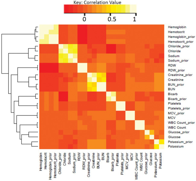
Heatmap of cross-sectional and longitudinal correlation. Shown is the correlation between various test results in our dataset when measured at the same time for the same patient and when measured at successive time points for the same patient. Analytes with the suffix “_prior” represent results from the analyte one measurement prior (within the same patient-admission) to analytes shown without this suffix. The dendrogram to the left of the heatmap represents the relative similarity between variables.

Assessment of 3D-MICE performance characteristics and prediction interval accuracy

Figures 5 and 6 summarize 3D-MICE performance for 2 representative but not necessarily best performing analytes: chloride and platelets (see Tables 2 and 3 and Figure 3 for specific analyte performance). The box plots (Figure 5) demonstrate a close association between measured and predicted values for both analytes and capture the uncertainty in predictions. The vertical overlap between boxes may serve as an indicator of the “resolution” of predicted values of the analyte in discriminating between various “ground truth” measured values of the analyte. The scatter plots (Figure 6) likewise demonstrate the association between measured and predicted values, but also demonstrate an association between prediction interval width and error. In particular, many data points with a high degree of error demonstrate the widest confidence intervals. Table 3 describes performance characteristics of 3D-MICE for all 13 analytes and the distribution of 95% prediction interval widths for all 13 analytes.

Figure 5.

Accuracy of chloride and platelet predictions and confidence intervals, box plots. Shown is the distribution of predicted results (vertical axis) corresponding to each range of measured results (horizontal axis). Horizontal lines within each box represent median values, boxes represent interpercentile ranges, and dots represent outliers. N’s represent the number of measured values falling within each range. (A) Chloride and (B) platelets are presented as 2 representative analytes.

Figure 6.

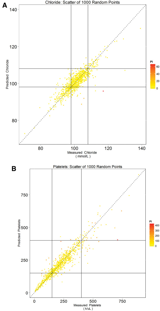
Accuracy of chloride and platelet predictions and confidence intervals, scatter plots. Predicted values for (A) chloride and (B) platelets are plotted as a function of measured values. Point colors represent prediction interval width. Horizontal and vertical lines represent the upper and lower normal reference limits. Note that less accurate predictions (points farther from the dashed 45-degree line) tend to be less confident, as indicated by the wider prediction interval and redder color.

Table 3.

Performance characteristics of 3D-MICE

Analyte (units)	Median absolute deviationb	Prediction interval widtha
		25th percentile	Median	75th percentile
	All values are expressed in the same units as the analyte
Chloride (mmol/L)	1.59	2.74	4.04	5.9
Potassium (mmol/L)	0.25	0.39	0.59	0.86
Bicarb (mmol/L)	1.42	2.32	3.48	4.94
Sodium (mmol/L)	1.44	2.47	3.59	5.02
Hematocrit (%)	0.83	1.38	2.35	3.65
Hemoglobin (g/dL)	0.27	0.47	0.79	1.24
MCV (fL)	0.82	1.26	1.92	2.85
Platelets (k/uL)	15.32	22.54	39.68	70.17
WBC count (k/uL)	1.13	1.59	2.86	5.03
RDW (%)	0.15	0.22	0.37	0.66
BUN (mg/dL)	1.79	3.09	5.17	8.75
Creatinine (mg/dL)	0.07	0.1	0.17	0.31
Glucose (mg/dL)	16.29	21.83	37.98	67.66

^aRepresents percentiles of the difference between the lower and upper bounds of the 95% prediction intervals. For example, 50% of predictions were made with a prediction interval width less than that shown in the median column.

^bThe median absolute deviation represents the median across all predictions for the analyte of the absolute value of the difference between the predicted and corresponding measured result; 50% of predictions differed from the measured result by less than the median absolute deviation.

Limitations

This study is subject to potential limitations. Foremost, we developed and applied 3D-MICE only in the context of selected routine tests on inpatients who met selected inclusion criteria. While >75% of all inpatient test results for the 13 analytes met the inclusion criteria, more than two-thirds of all inpatient admissions were excluded, primarily because they lacked enough data points. The inclusion criteria we applied are somewhat stricter than the minimum requirement to apply this algorithm in practice, since we needed to ensure sufficient data even after masking points for use in testing; in real applications, 3D-MICE could be performed without masking, and thus some cases excluded from this analysis could have 3D-MICE applied in the context of other applications. To better generalize 3D-MICE to a broader set of patients and data, we plan to explore future adaptations that use methods such as linear interpolations in place of GP for cases lacking sufficient temporal data to use 3D-MICE. Nonetheless, even in its current form and as discussed further below, 3D-MICE may provide a useful tool for temporal imputation in rich datasets such as those from patients with sufficient longitudinal or temporally dense data.

Another potential limitation is that imputation algorithm performance on masked data may not match the performance in imputing natively missing data. The decision to mask one test result per patient per analyte was not intended to mimic a common pattern of missing results in real clinical data. Indeed, the natively missing data necessarily represent the actual empiric distribution of missing data from our study set; the masked data were intended to generate additional missing data for which we had a ground truth for evaluation. In addition, the additionally introduced missing data (by masking) made the imputation task harder than our observed reality, and likely rendered our performance evaluation a conservative one. Additional work will be needed to fully validate the performance and suitability of this algorithm in addressing various clinical prediction challenges. Finally, the incremental improvement provided by 3D-MICE compared to MICE or GP alone was in some cases statistically significant yet modest in magnitude. We are nonetheless hopeful that this incremental improvement in performance will stimulate more research into better integration of cross-sectional and longitudinal imputation.

DISCUSSION AND FUTURE WORK

Here we demonstrate that 3D-MICE may provide a novel and practical approach to impute clinical laboratory time series data. While we demonstrate that 3D-MICE outperforms 2 established methods, MICE and GP-based imputation, it is difficult to directly compare our results to many other previously developed imputation strategies, including those noted in the related work section, due to differences in modeling assumption frameworks. As pointed out in the related work section, many prior imputation approaches focused on performing only cross-sectional or only longitudinal imputation. Most if not all previously published imputation approaches aimed at combining longitudinal and cross-sectional information either required regularly sampled time series (eg, tensor-based methods) or were unable to provide reliable estimates without more time points containing shared observations of multiple variables than would be available in clinical laboratory time series. An unusual but useful feature of 3D-MICE is that this algorithm requires neither regularly nor densely sampled time series. Additional work comparing 3D-MICE to imputation methods besides MICE and GP in head-to-head comparisons on datasets that satisfy the necessary assumptions may be informative. Additional work will also be useful to better understand the impact of dataset characteristics on imputation accuracy. Examples of dataset characteristics that may impact 3D-MICE performance could include frequency of test result intervals, type of inpatient admissions, and degree of patient care intensity.

Indeed, we foresee many applications for 3D-MICE. Foremost, we expect that 3D-MICE will provide a basis to impute missing longitudinal clinical data to enable the use of these data for subsequent computational analyses. Informaticians could use 3D-MICE to first “complete” clinical datasets and then apply machine. Given the comparatively strong performance of 3D-MICE across the composite of all analytes and with many individual analytes, it may represent a good starting point for laboratory imputation, and could perhaps be applied in combination with other imputation methods to address specific cases where other methods might outperform.

Another way to consider 3D-MICE involves the notion that laboratory test results usually serve as “noisy” indicators of the patient’s underlying clinical state, with noise introduced due to factors including pre-analytic, analytic, and biologic variability. Since the main goal of laboratory testing is usually not to obtain numeric test values in themselves, but rather to assess the patient’s underlying clinical status, we would suggest that an ideal test result prediction algorithm should predict the clinically relevant components of laboratory tests while disregarding the noise. Indeed, although we trained our algorithms to predict measured test results and assessed their performance accordingly, in some cases, predicted test results may better indicate the underlying clinical state than measured ones.¹⁵ In particular, multi-analyte–based predictions may benefit from a “regression to the mean” phenomenon, whereby measurement error and pre-analytic and biologic variability would be substantially independent and thus “average out.”

CONCLUSION

We describe and demonstrate 3D-MICE, a new algorithm for imputing longitudinal clinical laboratory test results across multiple analytes. We show that 3D-MICE can integrate cross-sectional and longitudinal imputation and will often provide more accurate predictions than either GP or MICE alone. We present these findings as a basis for future research to enhance 3D-MICE and apply it to other types of clinical and laboratory data. With additional work, we expect that 3D-MICE will provide an additional tool for use in clinical predictive analytic algorithms and clinical decision support.

Funding

This work was supported by a Massachusetts Institute of Technology–Massachusetts General Hospital strategic partnership grant provided under the “Grand Challenge I: Diagnostics.”

Competing Interests

The authors have no conflicts of interest to disclose.

Contributors

JB and YL developed the methods, designed the study, analyzed the data, and drafted the initial manuscript. All authors contributed to the project framework and design and participated in manuscript development.

References

- 1. Winslow RL, Trayanova N, Geman D, Miller MI. Computational medicine: translating models to clinical care. Sci Translational Med. 2012;4158:158rv11–58rv11. [DOI] [PMC free article] [PubMed] [Google Scholar]
- 2. Kohane IS. Ten things we have to do to achieve precision medicine. Science. 2015;3496243:37–38. [DOI] [PubMed] [Google Scholar]
- 3. Waljee AK, Mukherjee A, Singal AG et al. , Comparison of imputation methods for missing laboratory data in medicine. BMJ Open. 2013;38:e002847. [DOI] [PMC free article] [PubMed] [Google Scholar]
- 4. Weber GM, Adams WG, Bernstam EV et al. , Biases introduced by filtering electronic health records for patients with “complete data.” J Am Med Inform Assoc. 2017;246:1134–41. [DOI] [PMC free article] [PubMed] [Google Scholar]
- 5. Harel O, Zhou XH. Multiple imputation for the comparison of two screening tests in two-phase Alzheimer studies. Stat Med. 2007;2611:2370–88. [DOI] [PubMed] [Google Scholar]
- 6. Qi L, Wang YF, He Y. A comparison of multiple imputation and fully augmented weighted estimators for Cox regression with missing covariates. Stat Med. 2010;2925:2592–604. [DOI] [PMC free article] [PubMed] [Google Scholar]
- 7. Buuren S, Groothuis-Oudshoorn K. mice: Multivariate imputation by chained equations in R. J Stat Software. 2011;453:1–67. [Google Scholar]
- 8. Stekhoven DJ, Buhlmann P. MissForest: non-parametric missing value imputation for mixed-type data. Bioinformatics. 2012;281:112–18. [DOI] [PubMed] [Google Scholar]
- 9. Hastie T, Tibshirani R, Sherlock G, Eisen M, Brown P, Botstein D. Imputing Missing Data for Gene Expression Arrays. Stanford University Statistics Department technical report, 1999. [Google Scholar]
- 10. Raghunathan TE, Lepkowski JM, Van Hoewyk J, Solenberger P. A multivariate technique for multiply imputing missing values using a sequence of regression models. Survey Methodol. 2001;271:85–96. [Google Scholar]
- 11. Su Y-S, Gelman A, Hill J, Yajima M. Multiple imputation with diagnostics (mi) in R: opening windows into the black box. J Stat Software. 2011;452:1–31. [Google Scholar]
- 12. Hsu CH, Taylor JM, Murray S, Commenges D. Survival analysis using auxiliary variables via non-parametric multiple imputation. Stat Med. 2006;2520:3503–17. [DOI] [PubMed] [Google Scholar]
- 13. Little R, An H. Robust likelihood-based analysis of multivariate data with missing values. Statistica Sinica. 2004;14:949–68. [Google Scholar]
- 14. Long Q, Hsu C-H, Li Y. Doubly robust nonparametric multiple imputation for ignorable missing data. Statistica Sinica. 2012;22:149. [PMC free article] [PubMed] [Google Scholar]
- 15. Luo Y, Szolovits P, Dighe AS, Baron JM. Using machine learning to predict laboratory test results. Am J Clin Pathol. 2016;1456:778–88. [DOI] [PubMed] [Google Scholar]
- 16. Zhang G, Little R. Extensions of the penalized spline of propensity prediction method of imputation. Biometrics. 2009;653:911–18. [DOI] [PubMed] [Google Scholar]
- 17. Van Buuren S, Boshuizen HC, Knook DL. Multiple imputation of missing blood pressure covariates in survival analysis. Stats Med. 1999;186:681–94. [DOI] [PubMed] [Google Scholar]
- 18. Troyanskaya O, Cantor M, Sherlock G et al. , Missing value estimation methods for DNA microarrays. Bioinformatics. 2001;176:520–25. [DOI] [PubMed] [Google Scholar]
- 19. Deng Y, Chang C, Ido MS, Long Q. Multiple imputation for general missing data patterns in the presence of high-dimensional data. Sci Rep. 2016;6:21689. [DOI] [PMC free article] [PubMed] [Google Scholar]
- 20. Horton NJ, Kleinman KP. Much ado about nothing: a comparison of missing data methods and software to fit incomplete data regression models. Am Stat. 2007;611:79–90. [DOI] [PMC free article] [PubMed] [Google Scholar]
- 21. He Y, Yucel R, Raghunathan TE. A functional multiple imputation approach to incomplete longitudinal data. Stats Med. 2011;3010:1137–56. [DOI] [PMC free article] [PubMed] [Google Scholar]
- 22. Fast multivariate spatio-temporal analysis via low rank tensor learning. Adv Neural Inf Process Syst. 2014. [Google Scholar]
- 23. Accelerated online low rank tensor learning for multivariate spatiotemporal streams. Proceedings of the 32nd International Conference on Machine Learning. Lille, France: JMLR: W&CP volume 37; 2015. [Google Scholar]
- 24. Ge H, Caverlee J, Zhang N, Squicciarini A. Uncovering the spatio-temporal dynamics of memes in the presence of incomplete information. Proceedings of the 25th ACM International Conference on Information and Knowledge Management. Indianapolis: ACM; 2016:1493–502. [Google Scholar]
- 25. Chiou J-M, Zhang Y-C, Chen W-H, Chang C-W. A functional data approach to missing value imputation and outlier detection for traffic flow data. Transportmetrica B. 2014;22:106–29. [Google Scholar]
- 26. Kliethermes S, Oleson J. A Bayesian approach to functional mixed-effects modeling for longitudinal data with binomial outcomes. Stats Med. 2014;3318:3130–46. [DOI] [PMC free article] [PubMed] [Google Scholar]
- 27. Liu M, Taylor JM, Belin TR. Multiple imputation and posterior simulation for multivariate missing data in longitudinal studies. Biometrics. 2000;564:1157–63. [DOI] [PubMed] [Google Scholar]
- 28. Schafer JL, Yucel RM. Computational strategies for multivariate linear mixed-effects models with missing values. J Comput Graph Stat. 2002;112:437–57. [Google Scholar]
- 29. Hori T, Montcho D, Agbangla C, Ebana K, Futakuchi K, Iwata H. Multi-task Gaussian process for imputing missing data in multi-trait and multi-environment trials. Theor Appl Genet. 2016;12911:2101–15 [DOI] [PubMed] [Google Scholar]
- 30. Kolda TG, Bader BW. Tensor decompositions and applications. SIAM Rev. 2009;513:455–500. [Google Scholar]
- 31. Rasmussen CE. Gaussian processes in machine learning. In: Mendelson S, Smola AJ, eds. Advanced Lectures on Machine Learning. Berlin Heidelberg: Springer; 2004:63–71. [Google Scholar]
- 32. Bonilla EV, Chai KM, Williams C. Multi-task Gaussian process prediction. Advances in Neural Information Processing Systems 20 (NIPS); 2007. [Google Scholar]
- 33. Yu K, Tresp V, Schwaighofer A. Learning Gaussian processes from multiple tasks. Proceedings of the 22nd International Conference on Machine Learning; 2005:1012–19. ACM. [Google Scholar]
- 34. MacDonald B, Ranjan P, Chipman H. GPfit: an R package for Gaussian process model fitting using a new optimization algorithm. arXiv preprint arXiv:1305.0759. 2013. [Google Scholar]
- 35. Azur MJ, Stuart EA, Frangakis C, Leaf PJ. Multiple imputation by chained equations: what is it and how does it work? Int J Methods Psychiatr Res. 2011;201:40–49. [DOI] [PMC free article] [PubMed] [Google Scholar]
- 36. Warnes GR, Bolker B, Bonebakker L et al. , gplots: various R programming tools for plotting data. R Package Version. 2009;24:1. [Google Scholar]