Prediction of turbulence eddy dissipation of water flow in a heated metal foam tube

Abstract

The insertion of porous metal media inside the pipes and channels has already shown a significant heat transfer enhancement by experimental and numerical studies. Porous media could make a mixing flow and small-scale eddies. Therefore, the turbulence parameters are attractive in such cases. The computational fluid dynamics (CFD) approach can predict the turbulence parameters using the turbulence models. However, the CFD is unable to find the relation of the turbulence parameters to the boundary conditions. The artificial intelligence (AI) has shown potential in combination with the CFD to build high-performance predictive models. This study is aimed to establish a new AI algorithm to capture the patterns of the CFD results by changing the system’s boundary conditions. The ant colony optimization-based fuzzy inference system (ACOFIS) method is used for the first time to reduce time and computational effort needed in the CFD simulation. This investigation is done on turbulent forced convection of water through an aluminum metal foam tube under constant wall heat flux. The ANSYS-FLUENT CFD software is used for the simulations. The x and y of the fluid nodal locations, inlet temperature, velocity, and turbulent kinetic energy (TKE) are the inputs of the ACOFIS to predict turbulence eddy dissipation (TED) as the output. The results revealed that for the best intelligence of the ACOFIS, the number of inputs, the number of ants, the number of membership functions (MFs) and the rule are 5, 10, 93 and 93, respectively. Further comparison is made with the adaptive network-based fuzzy inference system (ANFIS). The coefficient of determination for both methods was close to 1. The ANFIS showed more learning and prediction times (785 s and 10 s, respectively) than the ACOFIS (556 s and 3 s, respectively). Finding the member function versus the inputs, the value of TED is calculated without the CFD modeling. So, solving the complicated equations by the CFD is replaced with a simple correlation.

Introduction

The transport phenomena and heat transfer within the permeable media are vital in several engineering applications such as membranes, packed-bed catalytic reactors, electronic cooling, and adsorption. Thermal management goal aims to ensure that each part’s temperature in a chemical/physical system remains within the definite operational domains^1,2, or to guarantee the improved enforced convective heat transfer in different applications such as heat exchangers, cooling towers, and solar collectors^3,4.

The utilization of metal froth-filled improved tubes is broadly examined in literature^5–7. Calmidi et al.⁸, Zhao et al.⁹, and Kim et al.¹⁰ conducted convection heat transfer implementation of metal foam-occupied channels with various structures experimentally and numerically to understand the underlying phenomena. The system’s parameters such as pore density, metal froth porosity, and channel geometry were extensively included affecting the fluid flow as well as heat transport. Moreover, Zhao et al.^11,12 assessed heat transfer and boiling flow in foam-filled horizontal metal tubes, where those elements affecting heat transfers and pressure drops were totally tested and studied.

Computational fluid dynamics (CFD) tools are commonly used to predict thermal and hydrodynamic parameters of convective flows^13,14. The CFD tools prevent the extra expenses of the experiments coming from the trial and error processes. However, the CFD approach has its own expenses, especially for complex cases (e.g. two-phase flows, turbulent flows, complicated geometries, etc.). Modeling such complicated cases require a lot of computational efforts and high-performance computers. Although the CFD method predicts the fluid flow characteristics (e.g. temperature, velocity, pressure, turbulence parameters, etc.), this approach cannot find the relationship of such parameters with each other at an accepted level.

Nowadays, scientists studied the effects of artificial intelligence (AI) algorithms on evaluating fluid characteristics to avoid solving complicated CFD cases and saving computational efforts. Once the CFD results are obtained, the AI algorithm can learn the data and find the general pattern of the CFD data changes. Besides, the AI algorithm can find the relationship between the flow characteristics. In new researches, a combination of Fuzzy Inference System (FIS) as the main core of intelligence with new meta-heuristic algorithms such as ant colony optimization, differential evolution, genetic, and particle swarm optimization algorithms were considered to study fluid dynamics and heat transfer. Changing in FIS parameters are important for achieving the best intelligence.

Recently some studies considered the contribution of the ANFIS (adaptive network-based fuzzy inference system) with the CFD to predict fluid flow characteristics^15–17. The studies just simply discussed the application of the ANFIS for the facilitation of the CFD. But there is no discussion about the details of the algorithm setup and the effect of using the other trainers (i.e. ant colony optimization, differential evolution, genetic, and particle swarm optimization algorithms). Besides, there are not any studies to present the ability of artificial intelligence for correlating fluid flow characteristics.

According to the above discussion, for filling the research gaps, this study tries to use the ant colony optimization-based fuzzy inference system (ACOFIS) method for the first time to help the CFD model by the reduction of the number of the simulations. The efficiency of ACOFIS is compared with the ANFIS. The heat transfer and hydrodynamics of water flow inside an aluminum metal foam tube exposed to a fixed heat transfer flux is selected as a case study. The simulation is done for several inlet velocities and inlet temperatures. The x and y of the fluid nodal locations, the temperature at the inlet (T), the velocity (V), and turbulent kinetic energy (TKE) are the inputs of the ACOFIS to predict turbulence eddy dissipation (TED) as the output. Finally, a correlation is developed for finding the values of TED as a function of x, y, T, V, and TKE.

Methodology

Geometry and boundary conditions

The geometry of the case study is a cylindrical tube with a diameter of 10 mm, and a length of 1 m. The fluid with uniform temperature of T₀ and uniform velocity of u₀ enters the pipe. It is assumed that the heat flux at the wall q_w is constant. The summary of the simulation cases and the boundary conditions are given in Table 1.

Table 1.

CFD cases.

Case no.	Wall (kW/m2)	Tinlet	Vinlet (m/s)
1	q = 95	295 k	0.91
2		305 k
3		325 k
4		335 k

CFD method

The assessment is carried out for fluid with the conditions: steady state, incompressible, 3D and turbulent regime within a tubular geometry completely occupied with porous material submerged with a one-phase Newtonian fluid. Furthermore, the introduced porous material in the tube is supposed homogenous and isotropic with a uniform permeability magnitude and porosity. The characteristics of porous media including material, porosity, permeability, and PPI are aluminum, 0.8, 5 × 10^–8 m², and 10, respectively. Moreover, temperature-caused change in the thermo-physical features of the solid matrix and the working fluid is considered negligible. Furthermore, it is assumed that viscous dissipation, natural convection gravitational effects, and radiation heat transfer will have an insignificant impact on temperature and velocity distributions as well as the solid and fluid are regarded in local thermodynamic equilibrium. The equations of mass, energy, and momentum conservations may be expressed as^18–22:

Continuity:

$$\frac{\partial \rho }{\partial t}+\mathrm{\nabla }·\left(\rho \overrightarrow{u}\right)=0$$ 1

Momentum:

$$\raisebox{1ex}{$1$}\!\left/ \!\raisebox{-1ex}{$\epsilon $}\right.\frac{\partial \rho \overrightarrow{u}}{\partial t}+\raisebox{1ex}{$1$}\!\left/ \!\raisebox{-1ex}{$\epsilon $}\right.\mathrm{\nabla }·\left(\rho \overrightarrow{u}\overrightarrow{u}\right)=-\mathrm{\nabla }p+\epsilon \rho \overrightarrow{g}+\raisebox{1ex}{$1$}\!\left/ \!\raisebox{-1ex}{$\epsilon $}\right.\mathrm{\nabla }\left[{\mu }_{}^e\left(\mathrm{\nabla }\overrightarrow{u}+{\left(\mathrm{\nabla }\overrightarrow{u}\right)}^T\right)\right]+\overrightarrow{F}$$ 2

F is given as:

$$\overrightarrow{F}=\left(\frac{{\mu }_f}{K}+\frac{{\rho }_{f}C\left|v\right|}{\sqrt{K}}\right)\overrightarrow{v}$$ 3

where K is the permeability and C is the inertial coefficient given as^23,24:

$$C=0.00212{\left(1-\epsilon \right)}^{-0.132}{\left(\frac{d_l}{d_p}\right)}^{-1.63}$$ 4

where d_l is the ligament and d_p is the pore size obtained as:

$$d_l=1.18d_p\sqrt{\frac{1-\epsilon }{3\pi }}\left(\frac{1}{1-e^{\raisebox{1ex}{$-\left(1-\epsilon \right)$}\!\left/ \!\raisebox{-1ex}{$0.04$}\right.}}\right)$$ 5

$$d_p=0.0254(m)/\omega (PPI)$$ 6

In Eq. (6), ω denotes pore density. Also, PPI stands for pores per inch.

Energy conservation equation:

$$\frac{\partial \rho H}{\partial t}+\mathrm{\nabla }·\left(\rho \overrightarrow{u_{}}H\right)=\mathrm{\nabla }\left[{\text{k}}_e\left(\mathrm{\nabla }T\right)\right]$$ 7

where effective thermal conductivity parameter is calculated as:

$$k_e=(1-\epsilon )k_s+\epsilon k_F$$ 8

where subscripts s and F refer to the solid and fluid, respectively.

The equations for water properties are written as²⁵:

Density:

$$\begin{array}{c}{\rho }_F=2446-20.674T+0.11576T^2-3.12895\times {10}^{-4}{T}^3+4.0505\times {10}^{-7}{T}^4-2.0546\times {10}^{-10}{T}^5\\ \\ \end{array}$$ 9

Viscosity:

$${\mu }_F=A{10}^{\left(\frac{B}{T-C}\right)}$$ 10

where A = 2.414 × 10–5, B = 247.8, and C = 140.

Specific heat:

$${\left(C_p\right)}_F=exp\left(\frac{8.29041-0.012557T}{1-\left(1.52373\times {10}^{-3}\right)T}\right)$$ 11

Turbulence modelling

The turbulence effect is simulated by the standard k–ɛ model reported by Launder and Spalding^26,27 as follows:

$$\frac{\partial }{\partial t}\left(\rho k\right)+\mathrm{\nabla }·(\rho k\overrightarrow{u})=\mathrm{\nabla }·\left[\left(\frac{{\mu }^t}{{\sigma }_k}\right)\mathrm{\nabla }(k_{})\right]+G-\rho \epsilon$$ 12

$$\frac{\partial }{\partial t}\left({\rho }_{}{\epsilon }_{}\right)+\mathrm{\nabla }·(\rho \epsilon \overrightarrow{u})=\mathrm{\nabla }·\left[\frac{{\mu }_{}^t}{{\sigma }_{\epsilon }}\mathrm{\nabla }\epsilon \right]+\frac{\epsilon }{k}(C_{1\epsilon }{G}_k-C_{2\epsilon }{\rho }_f\epsilon )$$ 13

$$G_{}={\mu }_t(\mathrm{\nabla }\overrightarrow{u_{}}+{(\mathrm{\nabla }\overrightarrow{u_{}})}^T)$$ 14

$${\mu }_t={\rho }_{}{C}_{\mu }\frac{k^2}{\epsilon }$$ 15

$$C_{\mu }=0.09,{\sigma }_k=1.00,{\sigma }_{\epsilon }=1.30,C_{1\epsilon }=1.44,C_{2\epsilon }=1.92$$

where G is the production of turbulence due to the liquid shear stress.

Numerical methods

All numerical methods, using in this study are available in the CFD package of ANSYS-Fluent. Fluent is finite volume (FV) scheme for converting the partial differential equations (PDEs) into algebraic equations for numerical solutions. Second-order upwind scheme is adopted for discretization of the momentum, energy, TKE and turbulent dissipation rate equations. SIMPLE algorithm is employed for the pressure–velocity coupling scheme. ANSYS Design Modeler is used for meshing process. The discretization grid is included 250, 10 and 50 nodes in the axial, radial and circumferential directions, respectively.

Ant colony optimization (ACO)

The artificial agents are used by the generic ACO algorithm cooperating to discover the decent solutions of continuous/discrete optimization tasks. In this optimization approach, the agents are termed ants mimicking searching performance of biological systems in discovering the shortest pathway to reach the source of food in nature. AS (Ant system)²⁸ is used for the Traveling Salesman Problem (TSP), in which the ants make solutions via an iterative manner, and produce a certain quantity of pheromone over the traveled pathways. Selecting the path is a stochastic process in terms of two parameters of the heuristic and pheromone values for a product. When ant k presently place at i city for TSP, selects city j with a probability as²⁹:

$$P_{\mathit{il}}^k=\frac{{[{\tau }_{\mathit{ij}}]}^{\alpha }{[\mathrm{\eta }]}^{\beta }}{\sum l\in N_i^k{[{\tau }_{\mathit{il}}]}^{\alpha }{[{\mathrm{\eta }}_{\mathit{il}}]}^{\beta }}ifj\in N_i^k$$ 16

In Eq. (16) α and β denote 2 modification parameters determining the relative significance between the heuristic in formation ${\mathrm{\eta }}_{\mathit{ij}}$, the pheromone trail ${\tau }_{\mathit{ij}}$, and $N_i^k$ is the asset of city contestants not met by the ant k. The pheromone value indicates the number of ants choosing the trail presently; however, the heuristic value is a problem-based quality action. Reaching a decision point, it probably selects the trail with the greater heuristic and pheromone values. When the ant reaches the destination, the equivalent solution to the path passed by the ant is assessed and the equivalent pheromone value on the pathway is updated as²⁹:

$${\tau }_{\mathit{ij}}\left(m,+,1\right)=\rho {\tau }_{\mathit{ij}}\left(m\right)+\sum _{k=1}^{\stackrel{\sim }{N}}\mathrm{\Delta }{\tau }_{\mathit{ij}}^k(m)$$ 17

where $\rho$ represents the pheromone trail perseverance and $\mathrm{\Delta }{\tau }_{\mathit{ij}}^k(m)$ shows the quantity of pheromone deposited by the ant k on the traversed arc ij. Stutzle et al.³⁰ indicated that the enhanced behavior could be attained by robust use of the best solutions, along with an operative mechanism to avoid initial search stagnation. It should be noted that despite numerous changes in the initial ant system to various problems, only fewer related reports³¹ exist on using ACO for estimating the parameters as detailed in this work.

Fuzzy inference system (FIS)

Fuzzy inference system (FIS) is a common computing framework in terms of the fuzzy set theory concepts, fuzzy reasoning, and fuzzy if–then rules. It was successfully utilized in fields like automatic control, data classification, computer vision, expert systems, and decision analysis. Three various kinds of fuzzy reasoning exist implementing Sugeno and Takagi if–then rules in FIS structure³². In this study, x- and y-direction, inlet temperature, turbulence kinetic energy (TKE) and velocity (V) are considered to acquire TED as output. The signals incoming are multiplied based on the AND rule. For instance, the ith rule’s function is³³:

$$w_i={\mu }_{\mathit{Ai}}\left(X\right){\mu }_{\mathit{Bi}}\left(Y\right){\mu }_{\mathit{Ci}}(Tin){\mu }_{\mathit{Di}}(\mathrm{TKE}){\mu }_{\mathit{Ei}}(\mathrm{V})$$ 18

where $w_i$ represent outcoming signal and ${\mu }_{\mathit{Ai}}$, ${\mu }_{\mathit{Bi}}$, ${\mu }_{\mathit{Ci}}$, ${\mu }_{\mathit{Di}}$ and ${\mu }_{\mathit{Ei}}$ denote the signals incoming from MFs run over the inputs x-direction (X), y-direction (Y), inlet temperature (T_in), TKE and velocity (V).

The relative value of each rule’s firing strength is obtained equal to the weight over the overall quantity of the firing strengths of all rules³³:

$$\stackrel{-}{w_i}=\frac{w_i}{\sum \left(w_i\right)}$$ 19

where $\stackrel{-}{w_i}$ denotes the normalized firing strength. The defuzzication step used the function of a consequence if–then rule provided by Takagi and Sugeno³².

Hence, the node function is³³:

$$\stackrel{-}{w_i}{f}_i=\stackrel{-}{w_i}(p_{i}X+q_{i}Y+r_{i}Tin+s_i\mathrm{TKE}+t_{i}V+u_i)$$ 20

where $p_i$, $q_i$, $r_i$, $s_i$, $t_i$, and $u_i$ denote the parameters of if–then rules.

Results and discussion

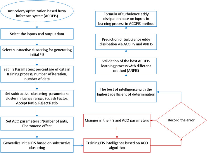
Figure 1 illustrates different steps of the fuzzy inference system (FIS) using the ant colony optimization (ACO) algorithm for learning the CFD results. Primarily, the inputs and the output of the ACOFIS are defined. The subtractive clustering is selected as the type of data clustering and for the inertia FIS. According to the CFD results, 2148 data are available for learning. The ACOFIS trains 70% of the CFD data for 60 iterations. The subtractive clustering parameters including the cluster influence range, the squash factor, the accept ratio, and the reject ratio are determined. For the ACO parameters, the number of ants and the pheromone effect are 10 and 0.2, respectively. Then the training process of the FIS is done based on the ACO algorithm. The TED predicted by the ACOFIS is compared with that predicted by the CFD. All errors of the ACOFIS predictions are calculated based on the CFD results. It should be noted that the values of ACO and FIS parameters are adjusted until the best intelligence is obtained. The sensitivity test for this adjustment is not considered in this study. The best intelligence of the ACOFIS is related to the highest coefficient of determination. Further validation is done by a comparison of the ACOFIS results with another artificial intelligence algorithm. This algorithm is also considered in this study for more comparison. In the end, the relation of the TED to the TKE and the inlet boundary conditions (velocity and temperature) is obtained. So, solving the complicated equations by the CFD is replaced with a simple correlation.

Figure 1.

Flowchart of ACOFIS method.

Table 2 summarized all parameters that have been adopted for the setup of ANFIS and ACOFIS parameters. According to Table 2, the values of all parameters are equal for both methods. The type of FIS, membership function, and clustering are also similar for both of them.

Table 2.

ACOFIS and ANFIS initial parameters.

Methods	ACOFIS	ANFIS
Number of inputs	5	5
Maximum of Iteration	60	60
Percentage of data in learning processes	70	70
Programming software	Matlab	Matlab
Type of FIS	Sugeno	Sugeno
Clustering type	Subtractive clustering	Subtractive clustering
Type of membership functions	Gaussmf	Gaussmf
Number of input membership function	94	111
Number of rules as FIS parameter	94	111
Cluster influence range as a subtractive clustering parameter	0.2	0.2
Squash factor as a subtractive clustering parameter	1.25	1.25
Accept ratio as a subtractive clustering parameter	0.5	0.5
Reject ratio as a subtractive clustering parameter	0.15	0.15
Number of ants as a ACO parameter	10	–
Pheromone effect as a ACO parameter	0.2	–

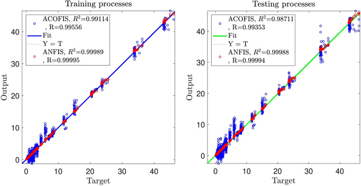
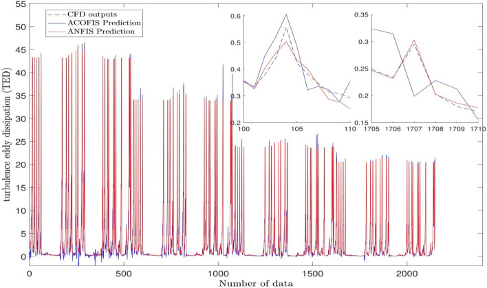
As shown in Fig. 2, the values of the correlation coefficient (R) and the coefficient of determination (R²) of the ANFIS (R = 0.99994 and R² = 0.99988) are a little higher than those of the ACOFIS (R = 0.99353 and R² = 0.98711). Figure 3 shows the prediction of the TED of both ANFIS and ACOFIS benchmarking the CFD results. Magnifying the graph, the ANFIS prediction shows a little more compatible results with the CFD than the ACOFIS. Table 3 shows a better comparison between the ANFIS and the ACOFIS. Based on the information of this table, for roughly the same values of R and R² for both methods, the ANFIS takes more learning and prediction times (785 s and 10 s respectively) than the ACOFIS (556 s and 3 s respectively).

Figure 2.

Regression plot of training and testing processes for the best FIS trained by ant colony optimization algorithm and the best result of ANFIS.

Figure 3.

Validation of ANFIS and ACOFIS prediction for prediction of turbulence eddy dissipation in each node.

Table 3.

ACOFIS and ANFIS different errors and learning and prediction times.

Methods	ACOFIS	ANFIS
Training correlation coefficient (R)	0.995558913	0.999947369
Training coefficient of determination (R2)	0.99113755	0.99989474
Testing correlation coefficient (R)	0.993532369	0.999941344
Testing coefficient of determination (R2)	0.987106569	0.999882692
Learning time (s)	555.8053779	785.4094361
Prediction time (s)	2.8730278	10.402829

The integration of the ACOFIS artificial intelligence with the CFD modeling in prediction of heat transfer and hydrodynamics of water flow through an Aluminum metal foam tube is investigated. The CFD modeling is done by ANSYS-FLUENT CFD software. The ACOFIS method uses the x and y of the fluid nodal locations, the temperature at the inlet (T), the velocity (V) and TKE as the inputs to predict TED as the output. Figure 4a,b show that the best intelligence could be obtained if all five inputs are included. Besides, the number of ants, and the number of membership functions (MFs) and the rule should be 10 and 93, respectively. According to Fig. 4, the regression number is roughly equal to 1 for both training and testing.

Figure 4.

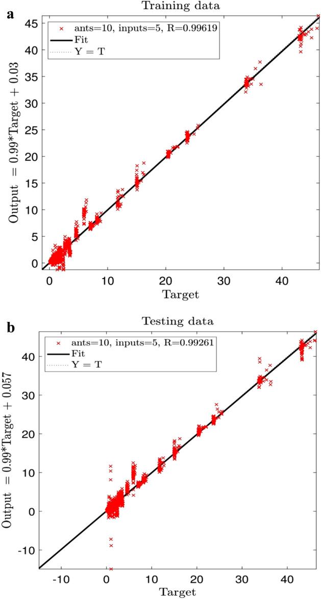
(a) Training process of ACOFIS using five inputs when number of ants is 10 and pheromone effect is 0.2. (b) Testing process of ACOFIS using five inputs when number of ants is 10 and pheromone effect is 0.2.

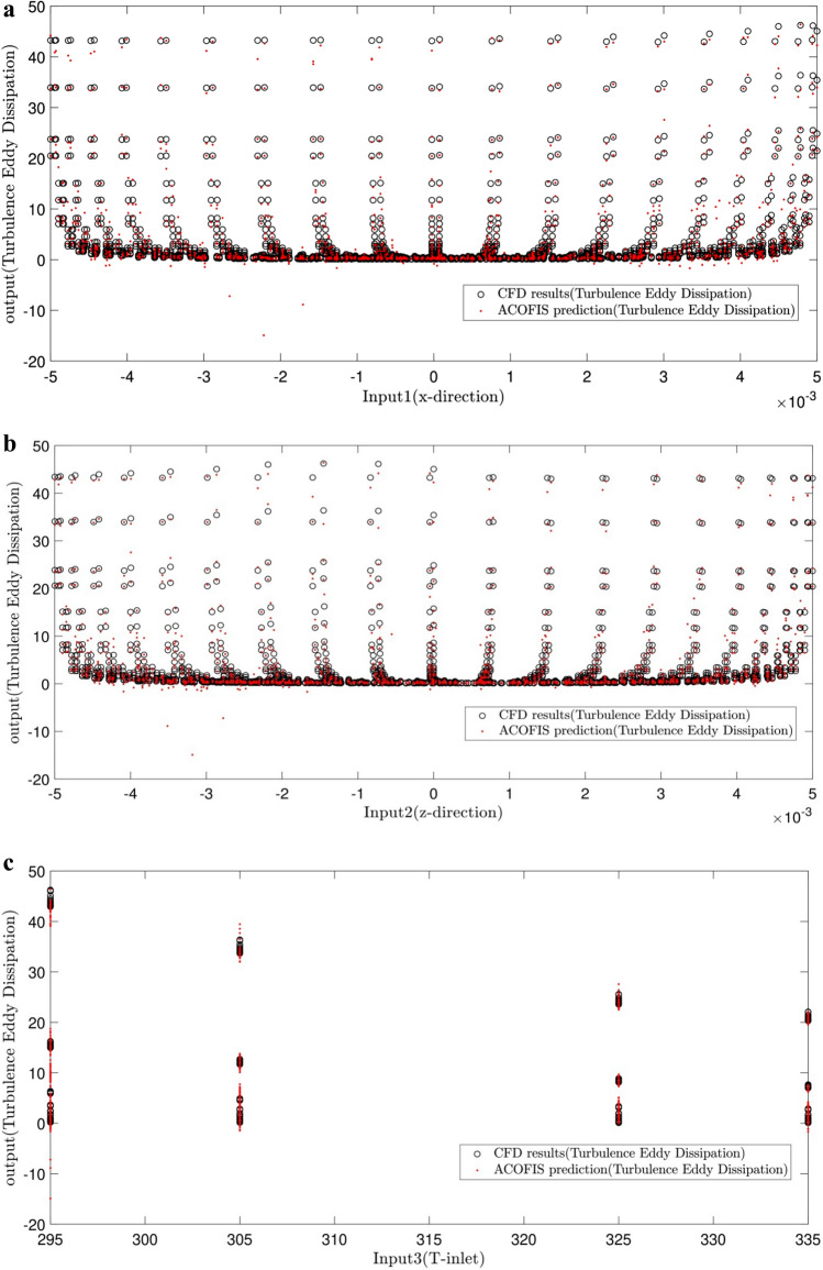
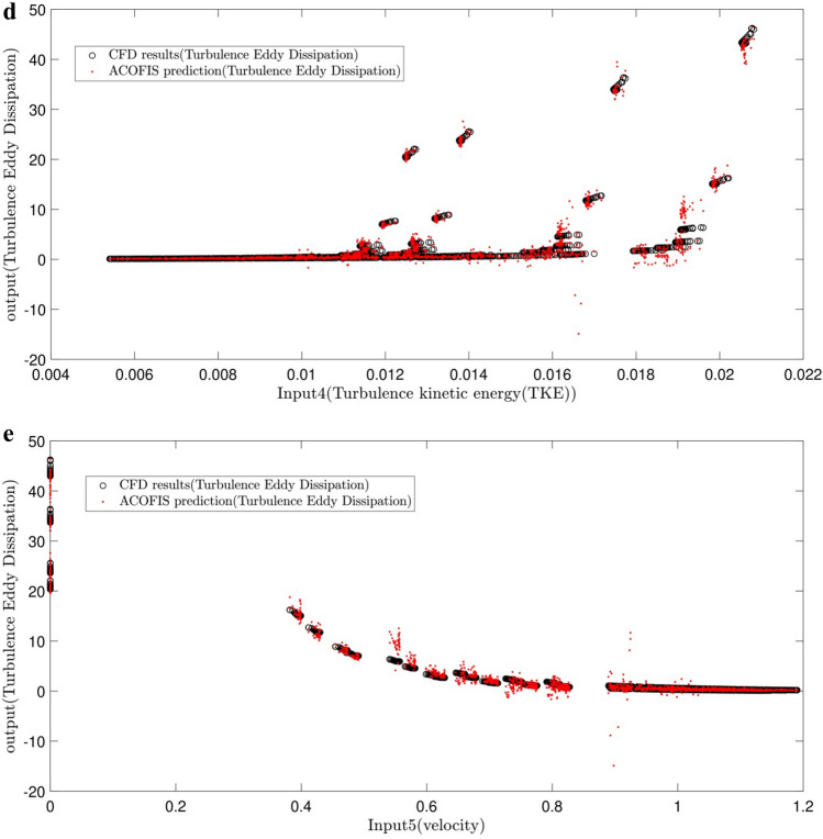
A comparative study is done between the CFD and the ACOFIS prediction of TED (shown in Fig. 5a–e). The results revealed that the predicted TED by the ACOFIS is in a good agreement with those by the CFD model for all 5 inputs.

Figure 5.

Comparison of ACOFIS output with CFD data (turbulence eddy dissipation) based on (a) x-direction as first input of ACOFIS, (b) y-direction as second input of ACOFIS, (c) inlet temperature as third input of ACOFIS, (d) Turbulence kinetic energy (TKE) as fourth input of ACOFIS, (e) velocity (V) as fifth input of ACOFIS.

The schematic diagram of the data clustering is illustrated by Fig. 6. The number of MFs for all inputs and the output, and the number of rules is equal to 93.

Figure 6.

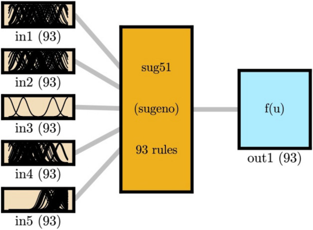
FIS structure trained by ACO algorithm as trainer in the highest level of intelligence.

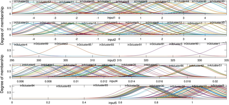
Figure 7 shows the degree of MFs for all inputs and all number of clustering. According to Fig. 7, the value of the Gaussian membership function can be determined for each value of the input. It should also be noted that there is a domain for all inputs. For example, the x and y are between ± 5 cm. The temperature limitation is from 295 to 335 K. The velocity must be selected from 0.006 to 0.02 m/s. The TKE is from 0 to 1 m²/s².

$$TED=\frac{{\sum }_{i=1}^{93}{\sum }_{j=1}^{93}{\sum }_{k=1}^{93}{\sum }_{l=1}^{93}{\sum }_{n=1}^{93}\left({\mu }_{1i},\times ,{\mu }_{2j},\times ,{\mu }_{3k},\times ,{\mu }_{4l},\times ,{\mu }_{5n}\right)\times \left(o_m,X,\times ,p_m,Y,\times ,q_m,T_{\mathit{inlet}},\times ,r_m,T,K,E,\times ,s_m,V,\times ,z_m\right)}{{\sum }_{i=1}^{93}{\sum }_{j=1}^{93}{\sum }_{k=1}^{93}{\sum }_{l=1}^{93}{\sum }_{n=1}^{93}\left({\mu }_{1i},\times ,{\mu }_{2j},\times ,{\mu }_{3k},\times ,{\mu }_{4l},\times ,{\mu }_{5n}\right)}$$ 21

in which

$${\mu }_{1i}=e^{\frac{-{\left(x,-,c_i\right)}^2}{2{\sigma }^2}},{\mu }_{2j}=e^{\frac{-{\left(x,-,c_j\right)}^2}{2{\sigma }^2}},{\mu 3k=e}^{\frac{-{\left(x,-,c_k\right)}^2}{2{\sigma }^2}},\mu 4l=e^{\frac{-{\left(x,-,c_l\right)}^2}{2{\sigma }^2}},\text{and}\mu 5n=e^{\frac{-{\left(x,-,c_n\right)}^2}{2{\sigma }^2}}$$

According to Eq. (21), turbulence eddy dissipation (TED) as the output is correlated to the x and y of the fluid nodal locations, the temperature at the inlet (T), the velocity (V), and TKE as the inputs. Table 4 shows the Gaussian function and its parameters.

Figure 7.

Degree of membership in the highest level of intelligence.

Table 4.

Gaussian membership function equation in ACOFIS learning process.

Membership function	Equation
Gaussian	$e^{\frac{-{\left(x,-,c\right)}^2}{2{\sigma }^2}}$

Table S1 (Supplementary Information) illustrates the values of C and σ as the parameters of Gaussian function at each cluster and for the best intelligence condition. Table S2 (Supplementary Information) illustrates consequent parameters (p, q, r, s, t, and u) at each cluster. After the determination of the value of the Gaussian membership function (µ), the value of TED is calculated by Eq. (21) without using the CFD. This leads to a lot of reduction in time and computational effort.

Conclusion

This study was aimed to offer a straightforward way for the reduction of the number of CFD simulations. This could be useful for complex cases like 3D geometries or turbulent flows. So, the 3D modeling of turbulent forced convection of water in a pipe was considered. In addition, the CFD approach is unable to find the relationship of the fluid flow parameters (i.e., velocity, temperature, turbulence parameters, etc.) with each other. This investigation aims to show the contribution of the ACOFIS artificial intelligence method, for the first time, in the prediction of heat transfer and hydrodynamics of water flow inside a metal foam tube. The ACOFIS was integrated with the CFD modeling. Once the CFD results are obtained, the ACOFIS can learn the data and find the general pattern of the CFD data changes.

The ANSYS-FLUENT CFD software was used for simulation of forced convection of water inside the metal foam tube. The water enters the tube by different inlet temperatures (i.e. 295, 305, 325 and 335 K). The x and y of the fluid nodal locations, the temperature at the inlet (T), the velocity (V), and turbulent kinetic energy (TKE) were considered as the inputs. The turbulence eddy dissipation (TED) was selected as the output. All the predictions were done on a cross-section in 0.3 m of the tube length. For more comparison, the efficiency of ACOFIS is compared with the adaptive network-based fuzzy inference system (ANFIS). The following results can be found from this investigation:

• The best intelligence (i.e. R ~ 1) could be obtained for the number of inputs equal to five. In addition, the number of ants, and the number of membership functions (MFs) and the rule should be 10 and 93, respectively.

• The comparative study between the CFD and the ACOFIS prediction of TED revealed that the predicted TED by the ACOFIS is in a good agreement with those by the CFD.

• The function of the degree of MFs versus all inputs and numbers of clustering was graphically determined. Once the values of the inputs are determined, the value of TED can be calculated without the CFD modeling. So, solving the complicated equations by the CFD could be replaced with a simple correlation.

• The coefficient of determination and the correlation of coefficient for both methods of ANFIS and ACOFIS were close to 1 at the best intelligence. The ANFIS showed more learning and prediction times (785 s and 10 s, respectively) than the ACOFIS (556 s and 3 s, respectively).

Author contributions

M.B.: simulations, writing-draft. I.B.: writing-draft, analysis. A.T.N.: writing-review, software, data analytics. M.R.: modeling, validation, revision. A.M.: funding, revision, validation, modeling. S.S.: supervision, funding, writing-review, conceptualization.

Competing interests

The authors declare no competing interests.

Supplementary information

is available for this paper at 10.1038/s41598-020-76260-6.

References

- 1.Hetsroni G, Mosyak A, Segal Z, Ziskind G. A uniform temperature heat sink for cooling of electronic devices. Int. J. Heat Mass Transf. 2002;45:3275–3286. doi: 10.1016/S0017-9310(02)00048-0. [DOI] [Google Scholar]
- 2.Nguyen Q, Babanezhad M, Taghvaie Nakhjiri A, Rezakazemi M, Shirazian S. Prediction of thermal distribution and fluid flow in the domain with multi-solid structures using Cubic-Interpolated Pseudo-Particle model. PLoS ONE. 2020;15:3850. doi: 10.1371/journal.pone.0233850. [DOI] [PMC free article] [PubMed] [Google Scholar]
- 3.Alkam M, Al-Nimr M. Solar collectors with tubes partially filled with porous substrates. ASME. 1999;121:20–24. [Google Scholar]
- 4.Nguyen Q, Taghvaie Nakhjiri A, Rezakazemi M, Shirazian S. Thermal and flow visualization of a square heat source in a nanofluid material with a cubic-interpolated pseudo-particle. ACS Omega. 2020;5(28):17658–17663. doi: 10.1021/acsomega.0c02173. [DOI] [PMC free article] [PubMed] [Google Scholar]
- 5.Astanina MS, Sheremet MA, Oztop HF, Abu-Hamdeh N. MHD natural convection and entropy generation of ferrofluid in an open trapezoidal cavity partially filled with a porous medium. Int. J. Mech. Sci. 2018;136:493–502. doi: 10.1016/j.ijmecsci.2018.01.001. [DOI] [Google Scholar]
- 6.Bhatti M, Khalique C, Bég TA, Bég OA, Kadir A. Numerical study of slip and radiative effects on magnetic Fe3O4-water-based nanofluid flow from a nonlinear stretching sheet in porous media with Soret and Dufour diffusion. Mod. Phys. Lett. B. 2020;34:2050026. doi: 10.1142/S0217984920500268. [DOI] [Google Scholar]
- 7.Waini I, Ishak A, Groşan T, Pop I. Mixed convection of a hybrid nanofluid flow along a vertical surface embedded in a porous medium. Int. Commun. Heat Mass Transf. 2020;114:104565. doi: 10.1016/j.icheatmasstransfer.2020.104565. [DOI] [Google Scholar]
- 8.Calmidi VV, Mahajan RL. Forced convection in high porosity metal foams. J. Heat Transf. 2000;122:557–565. doi: 10.1115/1.1287793. [DOI] [Google Scholar]
- 9.Zhao C, Kim T, Lu T, Hodson H. Thermal transport in high porosity cellular metal foams. J. Thermophys. Heat Transf. 2004;18:309–317. doi: 10.2514/1.11780. [DOI] [Google Scholar]
- 10.Kim, T., Fuller, A., Hodson, H. & Lu, T. An experimental study on thermal transport in lightweight metal foams at high Reynolds numbers. In Proceedings of Compact Heat Exchangers; A Festschrift on the 60th Birthday of Ramesh K. Shah, 227–232 (2002).
- 11.Zhao C, Lu W, Tassou S. Flow boiling heat transfer in horizontal metal-foam tubes. J. Heat Transf. 2009;131:121002. doi: 10.1115/1.3216036. [DOI] [Google Scholar]
- 12.Lu W, Zhao CY. Numerical modelling of flow boiling heat transfer in horizontal metal-foam tubes. Adv. Eng. Mater. 2009;11:832–836. doi: 10.1002/adem.200900139. [DOI] [Google Scholar]
- 13.Pishnamazi M, et al. Computational study on SO2 molecular separation applying novel EMISE ionic liquid and DMA aromatic amine solution inside microporous membranes. J. Mol. Liq. 2020;313:113531. doi: 10.1016/j.molliq.2020.113531. [DOI] [Google Scholar]
- 14.Babanezhad M, Nakhjiri AT, Marjani A, Shirazian S. Pattern recognition of the fluid flow in a 3D domain by combination of Lattice Boltzmann and ANFIS methods. Sci. Rep. 2020;10:1–13. doi: 10.1038/s41598-019-56847-4. [DOI] [PMC free article] [PubMed] [Google Scholar]
- 15.Nguyen Q, Behroyan I, Rezakazemi M, Shirazian S. Fluid velocity prediction inside bubble column reactor using ANFIS algorithm based on CFD input data. Arab. J. Sci. Eng. 2020;45:7487–7498. doi: 10.1007/s13369-020-04611-6. [DOI] [Google Scholar]
- 16.Tian E, Babanezhad M, Rezakazemi M, Shirazian S. Simulation of a bubble-column reactor by three-dimensional CFD: Multidimension-and function-adaptive network-based fuzzy inference system. Int. J. Fuzzy Syst. 2019;22:477–490. doi: 10.1007/s40815-019-00741-8. [DOI] [Google Scholar]
- 17.Pishnamazi M, et al. ANFIS grid partition framework with difference between two sigmoidal membership functions structure for validation of nanofluid flow. Sci. Rep. 2020;10:1–11. doi: 10.1038/s41598-019-56847-4. [DOI] [PMC free article] [PubMed] [Google Scholar]
- 18.Yang Y-T, Hwang M-L. Numerical simulation of turbulent fluid flow and heat transfer characteristics in heat exchangers fitted with porous media. Int. J. Heat Mass Transf. 2009;52:2956–2965. doi: 10.1016/j.ijheatmasstransfer.2009.02.024. [DOI] [Google Scholar]
- 19.Gangapatnam P, Kurian R, Venkateshan S. Numerical simulation of heat transfer in metal foams. Heat Mass Transf. 2018;54:553–562. doi: 10.1007/s00231-017-2149-6. [DOI] [Google Scholar]
- 20.Teamah MA, El-Maghlany WM, Dawood MMK. Numerical simulation of laminar forced convection in horizontal pipe partially or completely filled with porous material. Int. J. Therm. Sci. 2011;50:1512–1522. doi: 10.1016/j.ijthermalsci.2011.03.003. [DOI] [Google Scholar]
- 21.Babanezhad M, Nakhjiri AT, Rezakazemi M, Shirazian S. Developing intelligent algorithm as a machine learning overview over the big data generated by Euler–Euler method to simulate bubble column reactor hydrodynamics. ACS Omega. 2020;5:20558–20566. doi: 10.1021/acsomega.0c02784. [DOI] [PMC free article] [PubMed] [Google Scholar]
- 22.Babanezhad M, Nakhjiri AT, Shirazian S. Changes in the number of membership functions for predicting the gas volume fraction in two-phase flow using grid partition clustering of the ANFIS method. ACS Omega. 2020;5:16284–16291. doi: 10.1021/acsomega.0c02117. [DOI] [PMC free article] [PubMed] [Google Scholar]
- 23.Nield, D. A. & Bejan, A. In Convection in Porous Media 37–55 (Springer, Cham, 2017).
- 24.Nield, D. A. & Bejan, A. In Convection in Porous Media 57–84 (Springer, Cham, 2017).
- 25.Akbari M, Galanis N, Behzadmehr A. Comparative analysis of single and two-phase models for CFD studies of nanofluid heat transfer. Int. J. Therm. Sci. 2011;50:1343–1354. doi: 10.1016/j.ijthermalsci.2011.03.008. [DOI] [Google Scholar]
- 26.Launder BE, Spalding D. The numerical computation of turbulent flows. Comput. Methods Appl. Mech. Eng. 1974;3:269–289. doi: 10.1016/0045-7825(74)90029-2. [DOI] [Google Scholar]
- 27.Launder, B. E. & Spalding, D. B. In Numerical Prediction of Flow, Heat Transfer, Turbulence and Combustion, 96–116 (Elsevier, Amsterdam, 1983).
- 28.Dorigo M, Maniezzo V, Colorni A. Ant system: Optimization by a colony of cooperating agents. IEEE Trans. Syst. Man Cybern. Part B (Cybernetics) 1996;26:29–41. doi: 10.1109/3477.484436. [DOI] [PubMed] [Google Scholar]
- 29.Bell JE, McMullen PR. Ant colony optimization techniques for the vehicle routing problem. Adv. Eng. Inform. 2004;18:41–48. doi: 10.1016/j.aei.2004.07.001. [DOI] [Google Scholar]
- 30.Stützle T, Hoos HH. Max–Min ant system. Fut. Gen. Comput. Syst. 2000;16:889–914. doi: 10.1016/S0167-739X(00)00043-1. [DOI] [Google Scholar]
- 31.Nolle L. International Conference on Innovative Techniques and Applications of Artificial Intelligence. Berlin: Springer; 2007. pp. 3–16. [Google Scholar]
- 32.Takagi T, Sugeno M. Fuzzy identification of systems and its applications to modeling and control. IEEE Trans. Syst. Man Cybern. 1985;15:116–132. doi: 10.1109/TSMC.1985.6313399. [DOI] [Google Scholar]
- 33.Kim M-S, Kim C-H, Lee J-J. Evolving compact and interpretable Takagi–Sugeno fuzzy models with a new encoding scheme. IEEE Trans. Syst. Man Cybern. Part B (Cybernetics) 2006;36:1006–1023. doi: 10.1109/TSMCB.2006.872265. [DOI] [PubMed] [Google Scholar]
Associated Data
This section collects any data citations, data availability statements, or supplementary materials included in this article.