Modelling the role of optimal social distancing on disease prevalence of COVID-19 epidemic

Abstract

COVID-19 first spread from Wuhan, China in December 2019 but it has already created one of the greatest pandemic situations ever witnessed. According to the current reports, a situation has arisen when people need to understand the importance of social distancing and take enough precautionary measures more seriously. Maintaining social distancing and proper hygiene, staying at isolation or adopting the self-quarantine strategy are some common habits which people should adopt to avoid from being infected. And the growing information regarding COVID-19, its symptoms and prevention strategies help the people to take proper precautions. In this present study, we have considered a SAIRS epidemiological model on COVID-19 transmission where people in the susceptible environment move into asymptotically exposed class after coming contact with asymptotically exposed, symptomatically infected and even hospitalised people. The numerical study indicates that if more people from asymptotically exposed class move into quarantine class to prevent further virus transmission, then the infected population decreases significantly. The disease outbreak can be controlled only if a large proportion of individuals become immune, either by natural immunity or by a proper vaccine. But for COVID-19, we have to wait until a proper vaccine is developed and hence natural immunity and taking proper precautionary measures is very important to avoid from being infected. In the latter part, a corresponding optimal control problem has been set up by implementing control strategies to reduce the cost and count of overall infected individuals. Numerical figures show that the control strategy, which denotes the social distancing to reduce disease transmission, works with a higher intensity almost after one month of implementation and then decreases in the last few days. Further, the control strategy denoting the awareness of susceptible population regarding precautionary measures first increases up to one month after implementation and then slowly decreases with time. Therefore, implementing control policies may help to reduce the disease transmission at this current pandemic situation as these controls reduce the overall infected population and increase the recovered population.

Introduction

The very first case of novel Betacoronavirus was reported in December 2019 in Wuhan which is capital of Hubei Chinese province [1–3]. In the first few weeks, most of the cases were reported around wholesale Huanan seafood market of Wuhan where live animals are traded [4]. But surprisingly within almost five to six weeks, COVID-19 spread to all over the Chinese province and even across the world. World Health Organisation (WHO), observing the severity, declared COVID-19 as pandemic on March 17, 2020. The novel Coronavirus is an RNA virus from Coronaviridae family with order Nidovirales which is also known as SARS-CoV-2 [5, 6]. Viral pneumonia, fever, dry cough, aches and pains, tiredness, breathing problems etc. are the main symptoms of the disease [1, 7–9] though the recent report shows that loss of smell is another symptom of this disease. The estimated ‘case fatality ratio’ for the infection is of order 1% which makes it severe [10–13]. Hence, the virus has become a matter of concern in terms of public health priority as the virus is completely unknown to the human body and there is no pre-existing immunity present to resist the infection. According to the data of the dashboard provided by the Center for Systems Science and Engineering (CSSE) of John Hopkins University (JHU) and also from worldometers, the number of confirmed infected cases, documented death and recovery cases at June 15, 2020 have reached almost 8,034,461; 436,901 and 3,857,339 respectively across the world [14, 15]. Among 188 countries, United States (2,114,026 cases), Brazil (888,271 cases), Russia (536,484 cases), India (343,091 cases), UK (298,315 cases) are facing worse epidemic situations as the confirmed infected cases exceed 250,000 there. Particularly, the number of confirmed Coronavirus cases in the United States is highest as the virus spreads there at a very higher rate within a small time interval. The number of reported infected cases there increases from 15 to 2,114,026 till June 15, 2020. Also, US holds the top position in terms of death cases with number 116,127 but in case of recovery also, it has the highest number of cases with 576,334 recoveries. Quarantine strategy was first implemented in Wuhan, China on January 23, 2020 to control the situation and disease prevalence. According to the reports of June 15, 2020, China has 84,778 confirmed cases with the number of documented death and recovery are 4638 and 79,491 respectively. Observing the severity in China, other countries also call for complete or half national lockdown. France announced a lockdown on March 17 while United Kingdom announced on March 23 and even India called for lockdown on March 25. Observing the data and strategies, it looks like there is a large number of COVID-19 cases in India which are not registered due to lack of test kits. Moreover, recent reports reveal that there are many people shown positive result in COVID-19 test but they have not shown any kind of symptoms. So, these exposed asymptomatically infected individuals facilitate the spread of COVID-19 [2]. It is not the first time when zoonotic human Coronavirus invade in the population; in 2002, severe acute respiratory syndrome Coronavirus, known as SARS-CoV spread among 37 countries and in 2012, Middle East respiratory syndrome Coronavirus, known as MERS-CoV, spread among 27 countries.

In India, first COVID-19 case was confirmed at Kerala on January 30, 2020 when a student from Wuhan visited the state. According to NIC, India, there are total 343, 091 confirmed cases among which 153, 178 active cases, 180, 013 recoveries and 9, 900 death cases are reported in the country till June 15, 2020 [16, 17]. The Indian government has announced some vital precaution measures such as to maintain social distance, adopt the self-quarantine strategy, use a face mask, avoid touching faces frequently etc. so that large-scale disease transmission among the population can be avoided. In fact, when the number of affected cases crossed 500, the central government implemented a 14-hour long “Janata curfew" on March 22, 2020. Moreover, on March 24, the Government of India announced for a 21-days national lockdown from March 25 to April 14 to reduce the spread of COVID-19. But later, realizing the importance of the current pandemic situation, the duration of lockdown has been increased up to May 3, 2020 (Phase 2), then up to May 17, 2020 (Phase 3), then up to May 31, 2020 (Phase 4) and finally up to June 30, 2020 (Phase 5). With the fifth phase of lockdown, the Government has announced unlockdown 1.0 in some places where the contamination of the disease is below the risk level. Though the unlockdown comes with a long list of restrictions, reports of some sources reveal that daily average of cases and death calculated on weekly basis has been rising every single week for last 9-10 weeks. According to Worldometers and CSSE at JHU, India has come to position 4 right below of US, Brazil and Russia in terms of confirmed cases and even of recovery cases. On the very first day of unlockdown (June 1, 2020) India reaches to the peak till that date in terms of newly infected cases in a single day which is approximately 8392. Till June 15, 2020, India has a peak of 12,375 newly infected cases in a single day (which is reported on June 10). And the second peak was reported on June 13 with 12,023 newly infected cases per day [14, 15, 17]. As there is no vaccine is discovered yet, so, maintaining social distances or applying self-quarantine etc. are considered as the most effective prevention strategies [18]. People have been strictly instructed not to step out from homes except emergency and even if they go outside, then they have to maintain a safe distance and always have to carry face mask and hand sanitizer for hygiene purpose. The rules in lockdown include the closure of all shops except medical shops, hospitals, banks etc., suspension of all educational institutions and offices (only work–from–home and online classes are allowed), suspension of all medium of transport and also the prohibition on all social activities and gatherings. The lockdown strategy has helped to some extent actually. We wish to make slow down the rate of disease progression through lockdown. It has no doubt that Coronavirus pandemic has made a global impact in the past few months and continues to hit most of the sectors. This current outbreak has severely affected our day to day living both economically and health-wise. Reports from the World Bank and RBI state that this will be the first time after 1991 when the economic growth rate in India will be decreased by more than 1.5%–2.8% due to pandemic outbreak.

There are some literatures containing interesting statistical results about current COVID-19 outbreak [19–27]. Based on the data from December 31, 2019 to January 28, 2020, Wu et al. proposed an SEIR model for coronavirus transmission on both national and global range [28]. Also, Tang et al. [27] proposed a compartmental model for COVID-19 transmission with a combination of clinical development of the disease, current status of infected patients and control measures. According to their results, the control reproduction number may reach up to 6.47 and the implemented control policies minimize overall confirmed cases. A report submitted by Cambridge University reveals that India’s strategy of announcing 21–days lockdown may not be sufficient enough to prevent this pandemic outbreak in large scale and it can bounce back later that results in higher infection [29]. They suggested that the lockdown should be extended further into two or three phases with five-days or seven-days breaks in between or a single 49–days lockdown. Though India is currently under its fifth stage lockdown period which will continue up to 30th June.

In this manuscript, we have proposed a SAIRS epidemic model to describe Coronavirus transmission where it is considered that the susceptible population move into asymptomatically exposed class only after they come in touch with asymptomatically exposed, symptomatically infected and even hospitalised people. Also, a portion of the susceptible population may adopt precautionary measures from the very beginning so that they can directly move to recovered class. Population in India is almost 138 crores and so, it is hardly possible to call for complete lockdown across the country. Though a proportion of the susceptible population may take the precautionary measures successfully, the rest of the people is going to become infective (either asymptomatically exposed or symptomatically). Again the recovered people may move to susceptible class as permanent recovery is not guaranteed. The following two sections consist of the proposed epidemiological model for Coronavirus transmission and the positivity and boundedness of the system variables respectively. In Sect. 4, the basic reproduction number $(R_c)$ and equilibrium points of the proposed system are derived. Sensitivity analysis for some vital system parameters and stability analysis of the equilibria have been performed in Sects. 5 and 6 respectively. Sect. 7 consists of a theorem stating that the proposed system undergoes a forward bifurcation at $R_c=1$ around the disease-free equilibrium. The consequent section consists of the pictorial scenarios of the system dynamics without applying any control interventions. Later, a corresponding control problem has been set up to obtain optimal control interventions. Section 10 contains the numerical simulations of the system when the control strategies are implemented and the last section includes a brief conclusion.

Mathematical model: basic equations

In this work, we have proposed a compartmental epidemic model to analyse the effect of COVID-19 outbreak on the population worldwide. The total population N(t) at time t is divided into six subclasses such as susceptible population (S), asymptomatic individuals who have been exposed to the virus and have not yet been shown any clinical symptoms of COVID-19 (A), quarantined individuals (Q), symptomatically infected individuals (I), hospitalized and even isolated individuals (H) and recovered population (R). Individuals of the susceptible population become exposed when they come in contact with asymptomatically exposed or symptomatically infected people or even with hospitalised individuals through the term $({\beta }_{1}A+{\beta }_{2}I+{\beta }_{3}H)S$ where ${\beta }_1,{\beta }_2,{\beta }_3$ are the rates of disease transmission per contact by an asymptomatic exposed, symptomatic infected and hospitalised people respectively. The constant recruitment rate is denoted as $\mathrm{\Lambda }$ which is introduced in susceptible class. The term d denotes the natural death rate in all population whereas ${\delta }_1,{\delta }_2,{\delta }_3$ are disease-related death rates in asymptomatically exposed people, symptomatically infected and hospitalised individuals respectively. It is known that whether a person is infected by the virus or not can be detected by RT-PCR examination and according to some reports, a person with negative results in the test may still be a COVID-19 positive person as sometimes it takes about 7 to 14 days to develop symptoms in a body. Sometimes a person’s report turns out to be positive after two or three tests. Therefore, a portion of class A is considered as infected which considers the positive COVID-19 people. The people in the asymptomatically exposed class can move into either quarantine or symptomatic stage with rates p and $\eta$ respectively [30] depending on whether the asymptomatic people become cautious and take self-quarantine strategy or they develop symptoms at a very early stage. A quarantined individual is transferred into the hospitalised (including isolated) class at a rate of $\alpha$ depending on the development of clinical symptoms. The terms $\omega$ represents the progression rate from symptomatic to hospitalised stage. Also, $\xi$ and $\varphi$ are per-capita recovery rates for the quarantined and hospitalised individuals respectively. The recovery from the disease does not guarantee permanent recovery and so some of the recovered people move back to susceptible class further with rate constant $\psi$ [31]. To control the current pandemic situation and to spread awareness among individuals, the government have taken certain protective measures such as announcing lockdown, “Janata Curfew", spreading the information regarding social isolation and personal hygiene, implementing work from home policy during the lockdown etc. Though the government tries to spread necessary information, everyone does not become careful enough all the time and insufficient resources, poor financial condition, heedless nature etc. are some of the reasons in this case. A proportion of susceptible maintains the regulations and adopts behavioural changes seriously and moves to the recovered class at a rate $\kappa$.

So, the proposed model with positive parametric values takes the following form:

$$\begin{array}{cc}\hfill \frac{\mathit{dS}}{\mathit{dt}}& =\mathrm{\Lambda }-({\beta }_{1}A+{\beta }_{2}I+{\beta }_{3}H)S-dS+\psi R-\kappa S,\hfill \\ \hfill & S(0)>0,\hfill \\ \hfill \frac{\mathit{dA}}{\mathit{dt}}& =C+({\beta }_{1}A+{\beta }_{2}I+{\beta }_{3}H)S-pA-\eta A-(d+{\delta }_1)A,\hfill \\ \hfill & A(0)\ge 0,\hfill \\ \hfill \frac{\mathit{dQ}}{\mathit{dt}}& =pA-\alpha Q-\xi Q-dQ,Q(0)\ge 0,\hfill \\ \hfill \frac{\mathit{dI}}{\mathit{dt}}& =\eta A-\omega I-(d+{\delta }_2)I,I(0)\ge 0,\hfill \\ \hfill \frac{\mathit{dH}}{\mathit{dt}}& =\alpha Q+\omega I-\varphi H-(d+{\delta }_3)H,H(0)\ge 0,\hfill \\ \hfill \frac{\mathit{dR}}{\mathit{dt}}& =\kappa S+\xi Q+\varphi H-\psi R-dR,R(0)\ge 0,\hfill \\ \hfill \end{array}$$ 1

The model considers an average inflow of asymptomatic individuals into the system with a rate of C per unit time which includes immigration and emigration of individuals. There is a continuous inflow of travellers into the region during the COVID-19 outbreaks and because of the insufficient effective screening test, it may be assumed that some of these travellers are asymptomatically infected and enter into system at a rate C per day. For the sake of simplicity, C is considered as zero in this work. A schematic diagram has been provided in Fig. 1 to get a better insight into the proposed system.

Fig. 1.

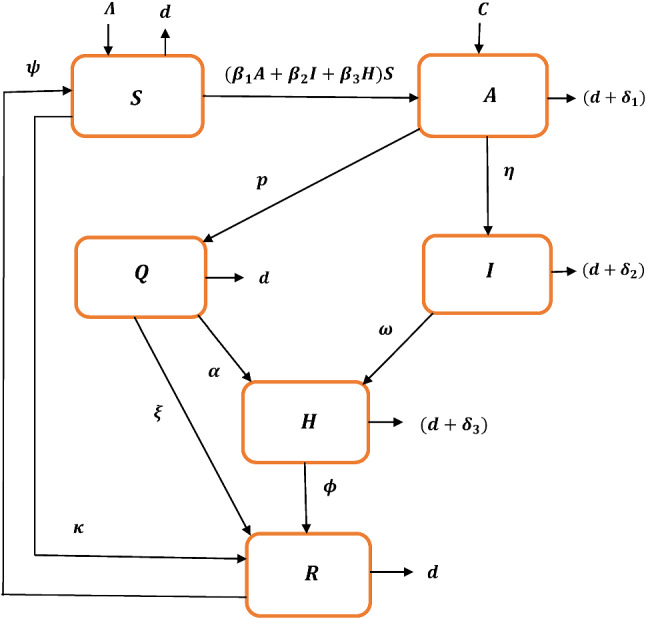
Schematic diagram of system (1)

Positivity and boundedness

For system (1): the following two theorems prove that the system variables are positive and bounded for all time. Proofs of the following two theorems are given in the Appendix.

Theorem 3.1

Solutions of system (1) starting from ${\mathbb{R}}_{+}^6$ are positive for all time.

Theorem 3.2

Solutions of system (1) which start from ${\mathbb{R}}_{+}^6$ are bounded for all $t>0$.

Equilibrium analysis

Solving the isoclines of model (1), we get that the system has (a) disease-free equilibrium point (DFE): ${\displaystyle E_0(S_0,0,0,0,0,R_0),}$ where ${\displaystyle S_0=\frac{\mathrm{\Lambda }(d+\psi )}{d(\kappa +\psi +d)}}$ and ${\displaystyle R_0=\frac{\mathrm{\Lambda }\kappa }{d(\kappa +\psi +d)},}$ and (b) endemic equilibrium point: $E^{\ast }(S^{\ast },A^{\ast },Q^{\ast },I^{\ast },H^{\ast },R^{\ast }).$

Basic reproduction number $(R_c)$

Basic reproduction number $R_c$ is the average number of newly infected individuals when they come in contact with a single infected person in susceptible environment. The method developed by van den Driessche and Watmough [32] is used here to determine $R_c$. In system (1), people from susceptible class move to asymptomatic class which is exposed to environment when they come in contact with asymptomatically infected (A), symptomatically infected (I) and hospitalised people (H). Let us take $x\equiv (A,Q,I,H)$. Let, ${\alpha }_0=p+\eta +d+{\delta }_1,{\alpha }_1=\alpha +\xi +d,{\alpha }_2=\omega +d+{\delta }_2$ and ${\alpha }_3=\varphi +d+{\delta }_3$. Second, third, fourth and fifth equations of model (1) can be written as:

$$\begin{array}{cc}\hfill \frac{\mathit{dx}}{\mathit{dt}}=& \mathfrak{F}(x)-\nu (x),\hfill \\ \hfill \mathfrak{F}(x)=& \left(\begin{array}{c}({\beta }_{1}A+{\beta }_{2}I+{\beta }_{3}H)S\\ 0\\ 0\\ 0\end{array}\right),\hfill \\ \hfill \nu (x)=& \left(\begin{array}{c}{\alpha }_{0}A\\ -pA+{\alpha }_{1}Q\\ -\eta A+{\alpha }_{2}I\\ -\alpha Q-\omega I+{\alpha }_{3}H\end{array}\right),\hfill \end{array}$$

where $\mathfrak{F}(x)$ contains only the compartment containing new infection term and $\nu (x)$ contains rest of the terms. So, corresponding linearized matrices of $\mathfrak{F}(x)$ and $\nu (x)$ at disease-free equilibrium $E_0=(S_0,0,0,0,0,R_0)$ are respectively

$$\begin{array}{cc}\hfill {\displaystyle F=}& \left(D,\mathfrak{F},(,x,)\right)(E_0)=\left(\begin{array}{cccc}{\beta }_1{S}_0& 0& {\beta }_2{S}_0& {\beta }_3{S}_0\\ 0& 0& 0& 0\\ 0& 0& 0& 0\\ 0& 0& 0& 0\end{array}\right);\hfill \\ \hfill V=& \left(D,\nu ,(,x,)\right)(E_0)=\left(\begin{array}{cccc}{\alpha }_0& 0& 0& 0\\ -p& {\alpha }_1& 0& 0\\ -\eta & 0& {\alpha }_2& 0\\ 0& -\alpha & -\omega & {\alpha }_3\end{array}\right)\hfill \end{array}$$

The spectral radius of next generation matrix $F{V}^{-1}$, denoted by $R_c$, is given by [32]:

$$\begin{array}{c}\hfill \begin{array}{cc}\hfill R_c& =\frac{S_0}{{\alpha }_0{\alpha }_1{\alpha }_2{\alpha }_3}[{\beta }_1{\alpha }_1{\alpha }_2{\alpha }_3+{\beta }_2\eta {\alpha }_1{\alpha }_3+{\beta }_3(p\alpha {\alpha }_2+\omega \eta {\alpha }_1)]\hfill \end{array}\end{array}$$ 2

Existence of endemic equilibrium point $E^{\ast }(S^{\ast },A^{\ast },Q^{\ast },I^{\ast },H^{\ast },R^{\ast })$

Consider, ${\alpha }_0=p+\eta +d+{\delta }_1,{\alpha }_1=\alpha +\xi +d,{\alpha }_2=\omega +d+{\delta }_2$ and ${\alpha }_3=\varphi +d+{\delta }_3$. From system (1) we have

$$\begin{array}{c}\hfill \begin{array}{cc}& \mathrm{\Lambda }-({\beta }_1{A}^{\ast }+{\beta }_2{I}^{\ast }+{\beta }_3{H}^{\ast })S^{\ast }-(d+\kappa )S^{\ast }+\psi R^{\ast }=0,\hfill \\ \hfill & ({\beta }_1{A}^{\ast }+{\beta }_2{I}^{\ast }+{\beta }_3{H}^{\ast })S^{\ast }-{\alpha }_0{A}^{\ast }=0\hfill \\ \hfill & p{A}^{\ast }-{\alpha }_1{Q}^{\ast }=0\hfill \\ \hfill & \eta A^{\ast }-{\alpha }_2{I}^{\ast }=0\hfill \\ \hfill & \alpha Q+\omega I-{\alpha }_3{H}^{\ast }=0\hfill \\ \hfill & \kappa S^{\ast }+\xi Q^{\ast }+\varphi H^{\ast }-(\psi +d)R^{\ast }=0.\hfill \end{array}\end{array}$$ 3

Solving these equations, we get ${\displaystyle S^{\ast }=\frac{S_0}{R_c},I^{\ast }=\frac{\mathrm{\Lambda }{\alpha }_1{\alpha }_3\eta (d+\psi )(1-\frac{1}{R_c})}{(d+\psi ){\alpha }_0{\alpha }_1{\alpha }_2{\alpha }_3-\psi \{p{\alpha }_2(\xi {\alpha }_3+\varphi \alpha )+\omega \eta \varphi {\alpha }_1\}},}$

$$\begin{array}{cc}\hfill {\displaystyle A^{\ast }=}& \frac{{\alpha }_2{I}^{\ast }}{\eta },Q^{\ast }=\frac{p{\alpha }_2{I}^{\ast }}{\eta {\alpha }_1},\hfill \\ \hfill H^{\ast }=& \frac{(p\alpha {\alpha }_2+\omega \eta {\alpha }_1)I^{\ast }}{\eta {\alpha }_1{\alpha }_3},R^{\ast }=\frac{\kappa S^{\ast }+\xi Q^{\ast }+\varphi H^{\ast }}{d+\psi }.\hfill \end{array}$$

Theorem 4.1

System (1) has a disease-free equilibrium $E_0\left(S_0,,,0,,,0,,,0,,,0,,,R_0\right)$ for any parametric values. Further,  for  $R_c>1,$ the system possesses a unique endemic equilibrium $E^{\ast }(S^{\ast },A^{\ast },Q^{\ast },I^{\ast },H^{\ast },R^{\ast })$ provided $(d+\psi ){\alpha }_0{\alpha }_1{\alpha }_2{\alpha }_3>\psi \{p{\alpha }_2(\xi {\alpha }_3+\varphi \alpha )+\omega \eta \varphi {\alpha }_1\}$.

Sensitivity analysis

For the proposed system, $R_c$ depends on some parameters like recruitment rate $(\mathrm{\Lambda })$, disease transmission rates $({\beta }_1,{\beta }_2,{\beta }_3),$ disease related death rates $({\delta }_1,{\delta }_2,{\delta }_3)$, natural mortality rate (d), progression rate of asymptomatic people into quarantine and infected classes $(p,\eta )$, probability at which recovered people move into susceptible classes $(\psi )$, progression rate of quarantined people and symptomatic infected population into hospitalised class $(\alpha ,\omega )$, progression rate of susceptible, quarantined and hospitalised population into recovered class $(\kappa ,\xi ,\varphi )$. Among all these parameters, we can control ${\beta }_1,{\beta }_2,{\beta }_3,p,\omega .$

Now, ${\displaystyle R_c=\frac{S_0}{{\alpha }_0{\alpha }_1{\alpha }_2{\alpha }_3}[{\beta }_1{\alpha }_1{\alpha }_2{\alpha }_3+{\beta }_2\eta {\alpha }_1{\alpha }_3+{\beta }_3(p\alpha {\alpha }_2+\omega \eta {\alpha }_1)],}$ where ${\displaystyle S_0=\frac{\mathrm{\Lambda }(d+\psi )}{d(\kappa +\psi +d)},{\alpha }_0=p+\eta +d+{\delta }_1,{\alpha }_1=\alpha +\xi +d,{\alpha }_2=\omega +d+{\delta }_2}$ and ${\alpha }_3=\varphi +d+{\delta }_3$. From the expression of $R_c$:

$$\begin{array}{c}\hfill \begin{array}{cc}\hfill \frac{\partial R_c}{\partial {\beta }_1}& =\frac{S_0}{{\alpha }_0}>0\hfill \\ \hfill \frac{\partial R_c}{\partial {\beta }_2}& =\frac{\eta S_0}{{\alpha }_0{\alpha }_2}>0\hfill \\ \hfill \frac{\partial R_c}{\partial {\beta }_3}& =\frac{S_0(p\alpha {\alpha }_2+\omega \eta {\alpha }_1)}{{\alpha }_0{\alpha }_1{\alpha }_2{\alpha }_3}>0\hfill \\ \hfill \frac{\partial R_c}{\partial p}& =-\frac{S_0[{\beta }_1{\alpha }_1{\alpha }_2{\alpha }_3+{\beta }_2\eta {\alpha }_1{\alpha }_3+{\beta }_3(p\alpha {\alpha }_2+\omega \eta {\alpha }_1)]}{{\alpha }_0^2{\alpha }_1{\alpha }_2{\alpha }_3}<0\hfill \\ \hfill \frac{\partial R_c}{\partial \omega }& =-\frac{S_0\eta ({\beta }_2{\alpha }_3+{\beta }_3\omega )}{{\alpha }_0{\alpha }_2^2{\alpha }_3}<0\hfill \\ \hfill \end{array}\end{array}$$

Next we compute normalized forward sensitivity index with respect to each of the parameters ${\beta }_1,{\beta }_2,{\beta }_3,p$ and $\omega$ to analyse the sensitivity of $R_c$ (to each of the parameters) by the method of Arriola and Hyman [33]:

$$\begin{array}{c}\hfill \begin{array}{cc}\hfill {\mathrm{\Theta }}_{{\beta }_1}& =\left|\frac{\frac{\partial R_c}{R_c}}{\frac{\partial {\beta }_1}{{\beta }_1}}\right|=\left|\frac{{\beta }_1}{R_c},\frac{\partial R_c}{\partial {\beta }_1}\right|\hfill \\ \hfill & =\left|\frac{{\beta }_1{\alpha }_1{\alpha }_2{\alpha }_3}{[{\beta }_1{\alpha }_1{\alpha }_2{\alpha }_3+{\beta }_2\eta {\alpha }_1{\alpha }_3+{\beta }_3(p\alpha {\alpha }_2+\omega \eta {\alpha }_1)]}\right|<1\hfill \\ \hfill {\mathrm{\Theta }}_{{\beta }_2}& =\left|\frac{\frac{\partial R_c}{R_c}}{\frac{\partial {\beta }_2}{{\beta }_2}}\right|=\left|\frac{{\beta }_2}{R_c},\frac{\partial R_c}{\partial {\beta }_2}\right|\hfill \\ \hfill & =\left|\frac{{\beta }_2\eta {\alpha }_1{\alpha }_3}{[{\beta }_1{\alpha }_1{\alpha }_2{\alpha }_3+{\beta }_2\eta {\alpha }_1{\alpha }_3+{\beta }_3(p\alpha {\alpha }_2+\omega \eta {\alpha }_1)]}\right|<1\hfill \\ \hfill {\mathrm{\Theta }}_{{\beta }_3}& =\left|\frac{\frac{\partial R_c}{R_c}}{\frac{\partial {\beta }_3}{{\beta }_3}}\right|=\left|\frac{{\beta }_3}{R_c},\frac{\partial R_c}{\partial {\beta }_3}\right|\hfill \\ \hfill & =\left|\frac{{\beta }_3(p\alpha {\alpha }_2+\omega \eta {\alpha }_1)}{[{\beta }_1{\alpha }_1{\alpha }_2{\alpha }_3+{\beta }_2\eta {\alpha }_1{\alpha }_3+{\beta }_3(p\alpha {\alpha }_2+\omega \eta {\alpha }_1)]}\right|<1\hfill \\ \hfill {\mathrm{\Theta }}_p& =\left|\frac{\frac{\partial R_c}{R_c}}{\frac{\partial p}{p}}\right|=\left|\frac{p}{R_c},\frac{\partial R_c}{\partial p}\right|=\left|\frac{p}{{\alpha }_0}\right|<1\hfill \\ \hfill {\mathrm{\Theta }}_{\omega }& =\left|\frac{\frac{\partial R_c}{R_c}}{\frac{\partial \omega }{\omega }}\right|=\left|\frac{\omega }{R_c},\frac{\partial R_c}{\partial \omega }\right|\hfill & \\ \hfill & =\left|\frac{\omega \eta {\alpha }_1({\beta }_2{\alpha }_3+{\beta }_3\omega )}{{\alpha }_2[{\beta }_1{\alpha }_1{\alpha }_2{\alpha }_3+{\beta }_2\eta {\alpha }_1{\alpha }_3+{\beta }_3(p\alpha {\alpha }_2+\omega \eta {\alpha }_1)]}\right|\hfill \\ \hfill \end{array}\end{array}$$

From the calculation, it is observed that the disease transmission rates ${\beta }_1,{\beta }_2$ and ${\beta }_3$ are directly proportional with basic reproduction number $R_c$. It is biologically acceptable as higher disease transmission rates increase the disease fatality. On the other hand, p represents the rate of quarantining of people who have been in contact with infected people. So, if more people enter to quarantine class, then it can reduce the probability of occurrence of a pandemic outbreak. Moreover, increasing $\omega$ reduce the disease prevalence and so, $\omega$ is inversely proportional with $R_c$. The calculations and numerical simulations reveal that $R_c$ is more sensitive to changes in ${\beta }_i$ for $i=1,2,3$ than p and $\omega$. So, if we try to reduce the transmission rates by maintaining social distances and taking proper precautions, then this epidemic situation may be handled.

Stability analysis

We discuss the local and global stability conditions for the disease-free equilibrium point as well as endemic equilibrium point in this section. Let, ${\alpha }_0=p+\eta +d+{\delta }_1,{\alpha }_1=\alpha +\xi +d,{\alpha }_2=\omega +d+{\delta }_2$ and ${\alpha }_3=\varphi +d+{\delta }_3$.

Local stability

The Jacobian matrix of system (1) is given as:

$$\begin{array}{c}\hfill \overline{J}=\left(\begin{array}{cccccc}-({\beta }_{1}A+{\beta }_{2}I+{\beta }_{3}H)-(d+\kappa )& -{\beta }_{1}S& 0& -{\beta }_{2}S& -{\beta }_{3}S& \psi \\ {\beta }_{1}A+{\beta }_{2}I+{\beta }_{3}H& {\beta }_{1}S-{\alpha }_0& 0& {\beta }_{2}S& {\beta }_{3}S& 0\\ 0& p& -{\alpha }_1& 0& 0& 0\\ 0& \eta & 0& -{\alpha }_2& 0& 0\\ 0& 0& \alpha & \omega & -{\alpha }_3& 0\\ \kappa & 0& \xi & 0& \varphi & -(d+\psi )\end{array}\right)\end{array}$$ 4

Theorem 6.1

DFE $(E_0)$ of system (1) is locally asymptomatically stable (LAS) for $R_c<1$ when $M_1,M_2,M_3>0$.

Proof

Proof is given in the Appendix. $\square$

Theorem 6.2

The endemic equilibrium point $E^{\ast }$ is LAS for $R_c>1$ when the conditions (i) $B_i>0$ for $i=1,6;$ and (ii) ${\mathrm{\Delta }}_i>0$ for $i=2,3,4,5$ hold.

Proof

Proof is given in the Appendix. $\square$

Global stability

To prove the global stability of DFE $E_0$, we use the method developed by Castillo-Chav$\acute{e}$z and Song [34]. Suppose a system is written as:

$$\begin{array}{c}\hfill \begin{array}{cc}\hfill \frac{\mathit{dX}}{\mathit{dt}}& =F(X,Y),\hfill \\ \hfill \frac{\mathit{dY}}{\mathit{dt}}& =G(X,Y),G(X,O)=O,\hfill \end{array}\end{array}$$ 5

where $X\in {\mathbb{R}}^{m_1}$ and $Y\in {\mathbb{R}}^{m_2}$ denote the uninfected and infected individuals respectively $(m_1,m_2\in {\mathbb{Z}}_{+})$. Consider $U_0=(X_0,O)$ as the DFE of system (5). Let us take two assumptions as:

(H1)

$X_0$ is globally asymptotically stable for ${\displaystyle \frac{\mathit{dX}}{\mathit{dt}}=F(X,O)}$.

(H2)

$G(X,Y)=D_{Y}G(X_0,O)Y-\overline{G}(X,Y),\overline{G}(X,Y)\ge O$ for $(X,Y)\in \mathrm{\Omega }$, where $\mathrm{\Omega }$ is a bounded invariant region and $D_{Y}G(X_0,O)$ is a stable matrix with non-negative off diagonal elements (i.e., an M-matrix).

If (H1) and (H2) hold for mentioned system (5), then the following theorem holds.

Theorem 6.3

The disease free equilibrium $U_0=(X_0,O)$ of the model system (5) is globally asymptotically stable (GAS) for $R_c<1$ if the conditions (H1) and (H2) hold.

Theorem 6.4

DFE $E_0$ of system (1), if LAS, is globally asymptotically stable (GAS) when $S\le S_0$ for $R_c<1$.

Proof

Proof is given in the Appendix. $\square$

Theorem 6.5

Endemic equilibrium point $E^{\ast }$ of system (1) is globally asymptomatically stable (GAS) when $\psi S^{\ast }{R}^{\ast }<2{\alpha }_0{S}^{\ast }{A}^{\ast }$ and $p{m}_2{\alpha }_2+\eta m_3{\alpha }_2+{\beta }_1{\alpha }_2{S}^{\ast }<{\alpha }_0{\alpha }_2$ hold in

$$\begin{array}{c}\hfill \begin{array}{cc}\hfill \mathrm{\Phi }& =\left\{(S,A,Q,I,H,R),\in ,{\mathbb{R}}_{+}^6,:,3,{\alpha }_0,A^{\ast },+,m_2,{\alpha }_1,Q^{\ast },+,m_3,{\alpha }_2,I^{\ast }\right)\hfill \\ \hfill & \left(+,m_4,{\alpha }_3,H^{\ast },<,{\beta }_1,A^{\ast },S,+,(d{R}^{\ast }-\kappa S),,\right)\hfill \\ \hfill & \left(S,<,S^{\ast },,,,d,R^{\ast },<,\kappa ,S\right\}.\hfill \end{array}\end{array}$$

where ${\alpha }_i$ for $i=0,1,2,3$ and $m_j$ for $j=1,2,3,4$ are mentioned in the proof.

Proof

Proof is given in the Appendix.

Bifurcation analysis at $R_c=1$

In order to establish the direction of bifurcation at the crucial threshold value $R_c=1,$ the central manifold theory is used as discussed in Castillo-Chav$\acute{e}$z and Song [34], and their result is stated in the following theorem:

Theorem 7.1

Consider the following system of ODEs with a parameter $\mathrm{\Psi }$:

$$\begin{array}{c}\hfill \frac{\mathit{dx}}{\mathit{dt}}=f(x,\mathrm{\Psi }),f:{\mathbb{R}}^n\times \mathbb{R}\to {\mathbb{R}}^{n}andf\in C^2\left({\mathbb{R}}^n,\times ,\mathbb{R}\right).\end{array}$$

For the system, O is taken as an equilibrium point and $f(O,\mathrm{\Psi })=O$ for all $\mathrm{\Psi }.$ Assume

• (I)$M=D_{x}f(O,0)=(\frac{\partial f_i}{\partial x_j}(O,0))$ is the linearization matrix of the system around the equilibrium O with $\mathrm{\Psi }$ evaluated at 0. M has a zero eigenvalue and other eigenvalues of M have negative real parts.
• (II)M has a non-negative right eigenvector w and a left eigenvector v corresponding to the zero eigenvalue.
  Let $f_k$ be the kth component of f and

  $$\begin{array}{cc}& a={\sum }_{k,i,j=1}^n{v}_k{w}_i{w}_j\frac{{\partial }^2{f}_k}{\partial x_i\partial x_j}(O,0),\hfill \\ \hfill & b={\sum }_{k,i=1}^n{v}_k{w}_i\frac{{\partial }^2{f}_k}{\partial x_i\partial \mathrm{\Psi }}(O,0),\hfill \end{array}$$

  Sign of a and b determine the local dynamical behaviour of a system around O.

  1. $a>0,b>0.$ If $\mathrm{\Psi }<0$ and $|\mathrm{\Psi }|\ll 1,$ then O is locally asymptotically stable and there exists a positive unstable equilibrium; when $0<\mathrm{\Psi }\ll 1,$ O is unstable and there exists a negative and locally asymptotically stable equilibrium.
  2. $a<0,b<0.$ If $\mathrm{\Psi }<0$ and $|\mathrm{\Psi }|\ll 1,$ then O is unstable; when $0<\mathrm{\Psi }\ll 1,$ O is locally asymptotically stable, and there exists a positive unstable equilibrium.
  3. $a>0,b<0.$ If $\mathrm{\Psi }<0$ and $|\mathrm{\Psi }|\ll 1,$ then O is unstable, and there exists a locally asymptotically stable negative equilibrium; when $0<\mathrm{\Psi }\ll 1,$ O is stable, and a positive unstable equilibrium appears.
  4. $a<0,b>0.$ If $\mathrm{\Psi }$ changes from negative to positive, then O changes its stability from stable to unstable. Correspondingly a negative unstable equilibrium becomes positive and locally asymptotically stable.

The non-negativity of components of the eigenvector w is not necessary if corresponding component of equilibrium is positive and has been mentioned as Remark 1 in [34].

The requirement that w is non-negative in the previous theorem is not necessary. When some components in w are negative, we still can apply the theorem, but one has to compare w with the equilibrium because the general parameterization of the center manifold before the coordinate change is ${\displaystyle W^{{\beta }_2}=\{x_0+{\beta }_2(t)y+k({\beta }_2,\mathrm{\Psi }):v·k({\beta }_2,\mathrm{\Psi }),|{\beta }_2|\le {\beta }_{2_0},{\beta }_2(0)=0\}}$ provided that $x_0$ is a non-negative equilibrium of system (usually $x_0$ is the DFE). Hence, $x_0-2\frac{b\mathrm{\Psi }}{a}>0$ requires that $w(j)>0$ whenever $x_0(j)=0.$ If $x_0(j)>0,$ then w(j) need not be positive.

Let us redefine $S=x_1,A=x_2,Q=x_3,I=x_4,H=x_5$ and $R=x_6$, then the system (1) can be rewritten as:

$$\begin{array}{c}\hfill \begin{array}{cc}\hfill \frac{d{x}_1}{\mathit{dt}}& =\mathrm{\Lambda }-({\beta }_1{x}_2+{\beta }_2{x}_4+{\beta }_3{x}_5)x_1-(d+\kappa )x_1+\psi x_6\equiv h_1,\hfill \\ \hfill \frac{d{x}_2}{\mathit{dt}}& =({\beta }_1{x}_2+{\beta }_2{x}_4+{\beta }_3{x}_5)x_1-{\alpha }_0{x}_2\equiv h_2,\hfill \\ \hfill \frac{d{x}_3}{\mathit{dt}}& =p{x}_2-{\alpha }_1{x}_3\equiv h_3,\hfill \\ \hfill \frac{d{x}_4}{\mathit{dt}}& =\eta x_2-{\alpha }_2{x}_4\equiv h_4,\hfill \\ \hfill \frac{d{x}_5}{\mathit{dt}}& =\alpha x_3+\omega x_4-{\alpha }_3{x}_5\equiv h_5,\hfill \\ \hfill \frac{d{x}_6}{\mathit{dt}}& =\kappa x_1+\xi x_3+\varphi x_5-(d+\psi )x_6\equiv h_6.\hfill \end{array}\end{array}$$ 6

We have considered $\mathrm{\Psi }={\beta }_2$ as bifurcation parameter for $R_c=1.$ Thus at $\mathrm{\Psi }={\mathrm{\Psi }}^{\ast }={\beta }_2^{\ast },R_c=1$ gives ${\displaystyle {\beta }_2^{\ast }=\frac{1}{\eta {\alpha }_1{\alpha }_3}\left[\frac{{\alpha }_0{\alpha }_1{\alpha }_2{\alpha }_3}{S_0},-,{\beta }_1,{\alpha }_1,{\alpha }_2,{\alpha }_3,-,{\beta }_3,(p\alpha {\alpha }_2+\omega \eta {\alpha }_1)\right].}$

The linearized matrix of the model system (6) at ${\displaystyle E_0\left(\frac{\mathrm{\Lambda }(d+\psi )}{d(d+\kappa +\psi )},,,0,,,0,,,0,,,0,,,\frac{\mathrm{\Lambda }\kappa }{d(d+\kappa +\psi )}\right)}$ with bifurcation parameter ${\beta }_2={\beta }_2^{\ast }$ is given by

$$\begin{array}{c}\hfill \overline{J}{|}_{E_0}=\left(\begin{array}{cccccc}-(d+\kappa )& -{\beta }_1{S}_0& 0& -{\beta }_2{S}_0& -{\beta }_3{S}_0& \psi \\ 0& {\beta }_1{S}_0-{\alpha }_0& 0& {\beta }_2{S}_0& {\beta }_3{S}_0& 0\\ 0& p& -{\alpha }_1& 0& 0& 0\\ 0& \eta & 0& -{\alpha }_2& 0& 0\\ 0& 0& \alpha & \omega & -{\alpha }_3& 0\\ \kappa & 0& \xi & 0& \varphi & -(d+\psi )\end{array}\right)\end{array}$$

Two eigenvalues are roots of the equation: ${\lambda }^2+(2d+\kappa +\psi )\lambda +d(\kappa +d+\psi )=0$ which imply that they are the roots with negative real parts and other four eigenvalues are roots of the following equation: ${\lambda }^4+M_1{\lambda }^3+M_2{\lambda }^2+M_3\lambda +M_4=0,$ where $M_1={\alpha }_0+{\alpha }_1+{\alpha }_2+{\alpha }_3-{\beta }_1{S}_0$, $M_2={\alpha }_0{\alpha }_2+{\alpha }_1{\alpha }_3+({\alpha }_0+{\alpha }_2)({\alpha }_1+{\alpha }_3)-{\beta }_1{S}_0({\alpha }_1+{\alpha }_2+{\alpha }_3)-{\beta }_2{S}_0\eta$, $M_3={\alpha }_0{\alpha }_2({\alpha }_1+{\alpha }_3)+{\alpha }_1{\alpha }_3({\alpha }_0+{\alpha }_2)-{\beta }_1{S}_0\{{\alpha }_1{\alpha }_3+{\alpha }_2({\alpha }_1+{\alpha }_3)\}-{\beta }_2{S}_0\eta ({\alpha }_1+{\alpha }_3)-{\beta }_3{S}_0(p\alpha +\omega \eta )$ and $M_4={\alpha }_0{\alpha }_1{\alpha }_2{\alpha }_3(1-R_c)$. So, $\overline{J}{|}_{E_0}({\beta }_2^{\ast })$ has a zero eigenvalue at $R_c=1$ as $M_4=0$ at $R_c=1$.

The right eigenvector corresponding to the zero eigenvalue of $\overline{J}{|}_{E_0}({\beta }_2^{\ast })$ is denoted by $w={(w_1,w_2,w_3,w_4,w_5)}^T$, where $w_1=-[{\alpha }_0{\alpha }_1{\alpha }_2{\alpha }_3(d+\psi )+p\xi \psi {\alpha }_2{\alpha }_3+\psi \varphi (p\alpha {\alpha }_2+\omega \eta {\alpha }_1)],w_2={\alpha }_1{\alpha }_2{\alpha }_3\{\kappa \psi +(d+\kappa )(d+\psi )\},w_3=p{\alpha }_2{\alpha }_3\{\kappa \psi +(d+\kappa )(d+\psi )\},w_4=\eta {\alpha }_1{\alpha }_3\{\kappa \psi +(d+\kappa )(d+\psi )\},w_5=(p\alpha {\alpha }_2+\omega \eta {\alpha }_1)\{\kappa \psi +(d+\kappa )(d+\psi )\}$ and $w_6=[(d+\kappa )\{(p\alpha {\alpha }_2+\omega \eta {\alpha }_1)+p\xi {\alpha }_2{\alpha }_3\}-\kappa {\alpha }_0{\alpha }_1{\alpha }_2{\alpha }_3].$ Also, the left eigenvector of $\overline{J}{|}_{E_0}({\beta }_2^{\ast })$ corresponding to zero eigenvalue is $v={(v_1,v_2,v_3,v_4,v_5)}^T$, where $v_1=0,v_2={\alpha }_1{\alpha }_2{\alpha }_3,v_3=\alpha {\alpha }_2{\beta }_3{S}_0,v_4={\alpha }_1{S}_0({\beta }_2{\alpha }_3+{\beta }_3\omega ),v_5={\alpha }_1{\alpha }_2{\beta }_3{S}_0$ and $v_6=0$. Hence

$$\begin{array}{c}\hfill \begin{array}{cc}\hfill a& =\sum _{k,i,j=1}^n{v}_k{w}_i{w}_j\frac{{\partial }^2{f}_k}{\partial x_i\partial x_j}(E_0)\hfill \\ \hfill & =2v_2{w}_1[{\beta }_1{w}_2+{\beta }_2{w}_4+{\beta }_3{w}_5]<0,\hfill \\ \hfill b& =\sum _{k,i=1}^n{v}_k{w}_i\frac{{\partial }^2{f}_k}{\partial x_i\partial \mathrm{\Psi }}(E_0)=v_2{w}_4{S}_0>0\hfill \end{array}\end{array}$$

Now, applying the last condition of Theorem 7.1, it is observed that the direction of bifurcation is forward.

Theorem 7.2

The DFE: $E_0$ changes its stability from stable to unstable at $R_c=1$ and system (1) undergoes a transcritical bifurcation around $E_0$ with bifurcation parameter ${\beta }_2={\beta }_2^{\ast }$ at $R_c=1.$

Numerical simulation without any control policy

Pictorial scenarios help us to understand system dynamics more clearly. The human population in India in June, 2020 is about 137.8 million, the annual birth rate is 18.2 births/1000 people and the annual death rate is 7.3 deaths/1000 people. So, we are taking $S(0)=1.378\times {10}^9$ and $\mathrm{\Lambda }=7\times {10}^4$ by applying unit conversion from year to day. And the death rate per day (d) we get is near about 0.00002. From the data provided in the dashboard by the centre for system science and engineering (CSSE) at John Hopkins University and also from the Worldometers database on $1^{\mathit{st}}$ June 2020, India has total 1, 98, 370 corona cases [14, 15]. And till the date, total activated cases, death cases and recovered cases are $97,008;5,608$ and 95, 754 respectively. Hence, unit conversion from month to day gives ${\delta }_3$ as $3\times {10}^{-3}$ and $\varphi$ as 0.0052. As total active cases till $1^{\mathit{st}}$ is 97, 008 among 1, 98, 370 cases; so, we get $(\alpha +\omega )$ as 0.0053 approximately [17]. So for the calculations, $\alpha$ and $\omega$ are taken as 0.0026 and 0.0027 respectively. According to the current epidemic situation of Coronavirus, the new human cases infected per unit day is denoted by $\beta SI\equiv ({\beta }_{1}A+{\beta }_{2}I+{\beta }_{3}H)S$. In April, total human cases infected by COVID-19 (I) is about 34, 863, the population in India (S) in May is approximately by $1.376\times {10}^9$, the new human cases $(\beta SI)$ in May is about 1, 55, 673 (which results in total 1, 90, 536 COVID-19 cases in May) [16, 17]. Hence, we have $({\beta }_1+{\beta }_2+{\beta }_3)\approx 7.44\times {10}^{-8}$ by doing the unit conversion from month to day. As per the data of $1^{\mathit{st}}$ June provided by Ministry of Health and Family Welfare, Government of India and previously mentioned database, the infected cases by COVID-19 is about 1, 55, 673 in May [14, 15, 17], so, for sake of simplicity I(0) is taken as approximately 5000, by doing the unit conversion from month to day. All the assumed and estimated parameters are listed in Table 1. Let us consider $A(0)=500,Q(0)={10}^3,H(0)={10}^3$ and $R(0)=4\times {10}^8$ to perform the numerical simulation in this section.

Table 1.

Parameter values used for numerical simulation of system (1)

Parametric values
$\mathrm{\Lambda }$	$7\times {10}^4$	${\beta }_1$	$4.5\times {10}^{-8}$
${\beta }_2$	$3.26995\times {10}^{-8}$	${\beta }_3$	$0.005\times {10}^{-10}$
d	0.00002	$\kappa$	0.6
$\psi$	0.001	p	0.45
$\eta$	0.3	$\alpha$	0.0026
${\delta }_1$	0.5	${\delta }_2$	0.006
${\delta }_3$	0.0003	$\omega$	0.0027
$\xi$	0.26	$\varphi$	0.0052

Figure 2 shows that for the parametric values in Table 1 and ${\beta }_2=3.26995\times {10}^{-10}$, the trajectory starting from mentioned initial point ultimately converges to DFE $E_0(5.9399\times {10}^6,0,0,0,0,3.4941\times {10}^9)$ and as we get the basic reproduction number $R_c$ as 0.26733 here which lies below unity, so, the disease cannot invade in the system in this case.

Fig. 2.

Stability of the populations around disease-free equilibrium $E_0$

Now if we start to increase the value of ${\beta }_2$, then for the mentioned value of ${\beta }_2$, i.e., for ${\beta }_2=3.26995\times {10}^{-8}$ along with parametric values in Table 1, the trajectory starting from mentioned initial point approaches to unique endemic equilibrium point $E^{\ast }(1.0684\times {10}^6,79366.72,135995.06,2.73\times {10}^6,1.3996\times {10}^6,6.7027\times {10}^8)$ with time (see Fig. 3). For these parametric values, we get $R_c=5.55962>1$ indicating the presence of infection in the system.

Fig. 3.

Stability of the populations around endemic equilibrium $E^{\ast }$

Now $E_0$ changes its stability when ${\beta }_2$ goes above a threshold value ${\beta }_{2[TC]}$ and becomes unstable for ${\beta }_2>{\beta }_{2[TC]}$. So, the system undergoes a transcritical bifurcation at ${\beta }_2={\beta }_{2[TC]}=4.8087\times {10}^{-9}$ around DFE $(E_0)$ (see Fig. 4).

Fig. 4.

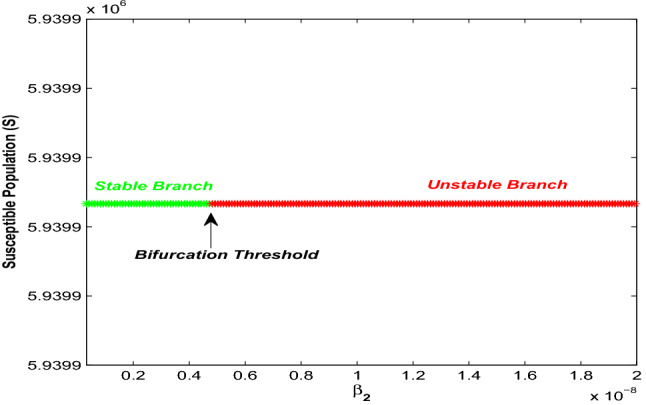
Trancritical bifurcation around $E_0$ taking ${\beta }_2$ as bifurcation parameter

Figure 5 demonstrates the sensibility of some of the vital parameters of the system on virus transmission. The figure shows that ${\beta }_2$ is most sensitive than ${\beta }_1$ and ${\beta }_3$ to control the disease transmission. A small increase of ${\beta }_2$ can increase the value of $R_c$ significantly. On the other hand, increasing value of p leads to a decrease in value of $R_c$, so if more people from asymptotically exposed class are quarantined, then the risk of contracting the disease decreases. Also, $\omega$ is inversely proportional with $R_c$, i.e., if more people admit to the hospitals without ignoring the symptoms, then the prevalence of the disease decreases with time.

Fig. 5.

Relationship between basic reproduction number $R_c$ with ${\beta }_1,{\beta }_2,{\beta }_3,p$ and $\omega$

Here, p denotes the rate at which asymptotically exposed people move into quarantine class. People become more cautious when the disease starts to outbreak at a higher rate and if more people are quarantined, then the spread of the disease decreases. Figure 6 shows the impact of the seriousness of being quarantined on the disease transmission especially on the infected population. According to this picture, more people moving into quarantine class can lower the count of infected population with time as the chance of interaction decreases for increasing p and people can successfully save themselves from getting infected. Also, if the susceptible individuals take the precautionary measures at a higher rate along with the increasing rate of entering quarantine class (from the class of asymptotically exposed people), then the infected population in the system decreases more. Figure 7 depicts that symptomatically infected population decrease significantly for increasing value of $\kappa$ for increasing p.

Fig. 6.

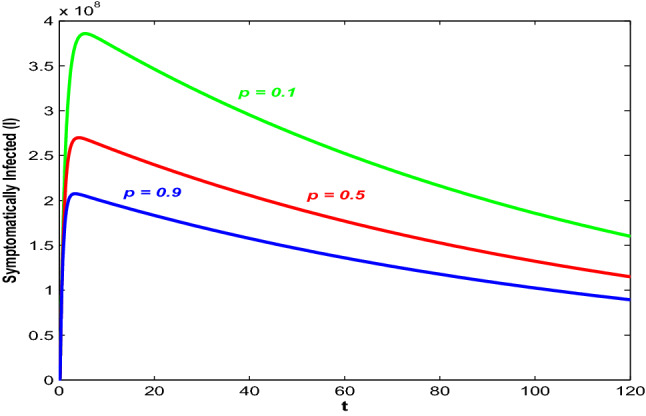
Trajectory profiles of symptomatically infected population (I) for different values of p

Fig. 7.

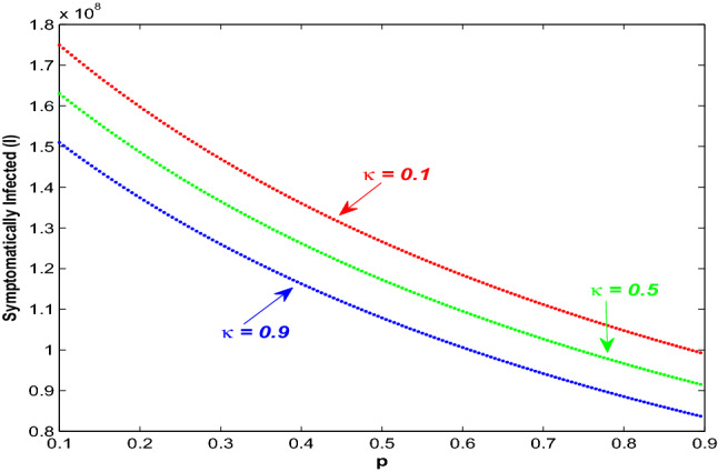
Variation of symptomatically infected population (I) due to change in rate of people being quarantined, p for different values of $\kappa$

Optimal control problem

We formulate the corresponding optimal control problem here to observe how suitable control interventions reduce the disease burden on the population. Maintaining social distancing to avoid the disease transmission at a higher rate and the precautions taken by susceptible to move to recovered class have been considered as the control policies. We have analysed analytically and also numerically how these control policies make their impact on disease transmission and try to optimize the cost burden for their implementations.

Increase the awareness among population for maintaining social distancing and proper hygiene: Population become aware of the severity of a disease and also of its prevention strategies from being infected when they are provided with sufficient information. The awareness programs and regular updates regarding COVID-19 act as important tools to increase the sensibility among the individuals. These days Government and media sources are spreading the news about this disease fatality regularly. COVID-19 is not an airborne disease and so people mainly become infected only when they come in touch with infected people both asymptomatically exposed and symptomatic individuals. So, maintaining social distancing in this pandemic situation plays a major role to reduce the disease fatality as social distancing reduces the average number of contacts. The virus of COVID-19 spread in a major portion of susceptible when they come into contact with an asymptotically exposed person and symptomatically infected person. It is assumed that $u_1$ portion of the susceptible population would maintain proper precautionary measures by using the face masks, keeping social distancing and implementing enough hygiene. Therefore, the disease can only be transmitted among $(1-u_1)S$ susceptible individuals due to the contact. In system (8), $u_1$ represents the intensity of maintaining social distancing in order to reduce the disease transmission with the restriction $0\le u_1\le 1$. Here, $u_1=0$ represents a full violation of social distancing and $u_1=1$ indicates full maintenance of social distancing. So, $u_1(t)$ changes according to the seriousness of the population regarding social distancing, we have taken this response intensity as one of the control variables. Incurred cost is involved as a non-linear function of $u_1$ to stimulate the response of individuals and regarding maintaining social distancing and applying home-quarantine strategy.

Due to the regular broadcast, a part of susceptible takes precautionary measures at a higher rate from the very beginning by maintaining proper hygiene, staying at isolation and even adopting the self-quarantine strategy. Thus this policy may be considered as one of the effective control tools and mainly the susceptible population of COVID-19 cases would be benefited by this policy. So, we are taking $u_2(t)$ as a control policy which denotes the intensity at which susceptible people move to recovered class directly by taking protective measures from beginning satisfying $0\le u_2(t)\le 1$.

The main work is to determine optimal response intensity and optimal treatment with minimum cost by the help of provided information. So, the region for the control interventions $u_1(t)$ and $u_2(t)$ is given as:

$$\begin{array}{c}\hfill \mathrm{\Pi }=\left\{\left(u_1,(t),,,u_2,(t)\right),|,\left(u_1,(t),,,u_2,(t)\right),\in ,[0,1],\times ,[0,1],,,t,\in ,[0,T_f]\right\},\end{array}$$

where $T_f$ is the final time upto which the control policies are executed, and also $u_i(t)$ for $i=1,2$ are measurable and bounded functions.

Determination of total cost

We determine the incurred cost which needs to be minimized in order to apply control interventions.

Cost incurred in maintaining social distancing and proper hygiene: The total cost incurred due to maintaining social distancing and proper hygiene is given as:

$$\begin{array}{c}\hfill {\int }_0^{T_f}\left[w_1,A,(t),+,w_2,I,(t),+,w_3,u_1^2,(t),+,w_4,u_2^2,(t)\right]dt\end{array}$$

The cost for spreading awareness regarding precautions and prevention measures among population by maintaining social distance, home-quarantine and hygiene via social campaigns, media etc. is denoted by $w_{1}A(t)+w_{2}I(t)+w_3{u}_1^2(t)+w_4{u}_2^2(t)$. The term considers the cost of associated efforts to convince the individuals about the importance of maintaining social distances and proper hygiene (by using face masks and sanitizer etc.) and it is observed that this cost is high enough. Also, the term considers the productivity loss due to home quarantine or isolation and also due to illness. There are some literatures that reveal the impact of the cost associated with awareness programs, screening and self-protective measures and non-linearity up to order two have been recommended [35–37]. We, in this work, now emphasize on the fact how social distancing and maintaining hygiene reduce the disease burden at the time of this pandemic outbreak.

The following control problem is considered based on previous discussions along with the cost functional J to be minimized:

$$\begin{array}{cc}& J[u_1(t),u_2(t)]\hfill \\ \hfill & ={\int }_0^{T_f}\left[w_1,A,(t),+,w_2,I,(t),+,w_3,u_1^2,(t),+,w_4,u_2^2,(t)\right]dt\hfill \end{array}$$ 7

subject to the model system:

$$\begin{array}{c}\hfill \begin{array}{cc}\hfill \frac{\mathit{dS}}{\mathit{dt}}& =\mathrm{\Lambda }-(1-u_1(t))({\beta }_{1}A+{\beta }_{2}I)S\hfill \\ \hfill & -{\beta }_{3}HS-dS+\psi R-u_2(t)S,\hfill \\ \hfill \frac{\mathit{dA}}{\mathit{dt}}& =(1-u_1(t))({\beta }_{1}A+{\beta }_{2}I)S+{\beta }_{3}HS-{\alpha }_{0}A,\hfill \\ \hfill \frac{\mathit{dQ}}{\mathit{dt}}& =pA-{\alpha }_{1}Q,\hfill \\ \hfill \frac{\mathit{dI}}{\mathit{dt}}& =\eta A-{\alpha }_{2}I,\hfill \\ \hfill \frac{\mathit{dH}}{\mathit{dt}}& =\alpha Q+\omega I-{\alpha }_{3}H,\hfill \\ \hfill \frac{\mathit{dR}}{\mathit{dt}}& =u_2(t)S+\xi Q+\varphi H-(d+\psi )R\hfill \end{array}\end{array}$$ 8

with initial conditions $S(0)>0,A(0)\ge 0,Q(0)\ge 0,I(0)\ge 0,H(0)\ge 0$ and $R(0)\ge 0.$ Here ${\alpha }_0=(p+\eta +d+{\delta }_1),{\alpha }_1=\alpha +\xi +d,{\alpha }_2=\omega +d+{\delta }_2$ and ${\alpha }_3=\varphi +d+{\delta }_3$. The functional J denotes the total incurred cost as stated and the integrand:

$$\begin{array}{cc}& L(S,A,Q,I,H,R,u_1(t),u_2(t))\hfill \\ \hfill & =w_{1}A(t)+w_{2}I(t)+w_3{u}_1^2(t)+w_4{u}_2^2(t)\hfill \end{array}$$

denotes the cost at time t. Positive parameters $w_1,w_2,w_3\text{and}{w}_4$ are weight constants balancing the units of the integrand [36, 38]. The optimal control interventions $u_1^{\ast }$ and $u_2^{\ast }$, exist in $\mathrm{\Pi }$, mainly minimize the cost functional J.

Theorem 9.1

The optimal control interventions $u_1^{\ast }$ and $u_2^{\ast }$ in $\mathrm{\Pi }$ of the control system (7)-(8) exist such that $J(u_1^{\ast },u_2^{\ast })=min[J(u_1,u_2)]$.

Proof

Proof is done in Appendix. $\square$

Pontryagin’s Maximum Principle helps to obtain optimal controls $u_1^{\ast }$ and $u_2^{\ast }$ of system (7)-(8).

Theorem 9.2

If $u_1^{\ast }$ and $u_2^{\ast }$ are the optimal controls and $S^{\ast },A^{\ast },Q^{\ast },I^{\ast },H^{\ast },R^{\ast }$ are corresponding optimal states of the control system (7)-(8), then there exist adjoint variables $\lambda =\left({\lambda }_1,,,{\lambda }_2,,,\dots ,,,{\lambda }_6\right)\in {\mathbb{R}}^6$ satisfying the canonical equations:

$$\begin{array}{c}\hfill \begin{array}{cc}\hfill \frac{d{\lambda }_1}{\mathit{dt}}& ={\lambda }_1[({\beta }_{1}A+{\beta }_{2}I)(1-u_1)+{\beta }_{3}H+u_2+d]\hfill \\ \hfill & -{\lambda }_2[({\beta }_{1}A+{\beta }_{2}I)(1-u_1)+{\beta }_{3}H]-{\lambda }_6(u_2)\hfill \\ \hfill \frac{d{\lambda }_2}{\mathit{dt}}& =-w_1+{\lambda }_1[(1-u_1){\beta }_{1}S]-{\lambda }_2[(1-u_1){\beta }_{1}S\hfill \\ \hfill & -{\alpha }_0]-{\lambda }_3(p)-{\lambda }_4(\eta )\hfill \\ \hfill \frac{d{\lambda }_3}{\mathit{dt}}& ={\lambda }_3({\alpha }_1)-{\lambda }_5(\alpha )-{\lambda }_6(\xi )\hfill \\ \hfill \frac{d{\lambda }_4}{\mathit{dt}}& =-w_2+{\lambda }_1[(1-u_1){\beta }_{2}S]-{\lambda }_2[(1-u_1){\beta }_{2}S]\hfill \\ \hfill & +{\lambda }_4({\alpha }_2)-{\lambda }_5(\omega )\hfill \\ \hfill \frac{d{\lambda }_5}{\mathit{dt}}& ={\lambda }_1({\beta }_{3}S)-{\lambda }_2({\beta }_{3}S)+{\lambda }_5({\alpha }_3)-{\lambda }_6(\varphi )\hfill \\ \hfill \frac{d{\lambda }_6}{\mathit{dt}}& =-{\lambda }_1(\psi )+{\lambda }_6(d+\psi )\hfill \end{array}\end{array}$$ 9

with transversality conditions ${\lambda }_i(T_f)=0$ for $i=1,2,\dots ,6$. The corresponding optimal controls $u_1^{\ast }$ and $u_2^{\ast }$ are given as:

$$\begin{array}{c}\hfill \begin{array}{cc}\hfill u_1^{\ast }& =min\left\{max,\left\{0,,,\left(\frac{({\beta }_1{A}^{\ast }+{\beta }_2{I}^{\ast })S^{\ast }}{2w_3},\left({\lambda }_2,-,{\lambda }_1\right)\right)\right\},,,1\right\},\hfill \\ \hfill u_2^{\ast }& =min\left\{max,\left\{0,,,\left(\frac{S^{\ast }}{2w_4},\left({\lambda }_1,-,{\lambda }_6\right)\right)\right\},,,1\right\}.\hfill \end{array}\end{array}$$ 10

Proof

Proof is given in Appendix. $\square$

Numerical results with control policies

In system (8), different control strategies have been implemented to reduce the disease burden and to minimize the total cost by finding the optimal control paths. Social distancing and maintaining proper hygiene vary with time because it depends on disease prevalence and also disease fatality. So, $u_1$ and $u_2$ are taken as a control variables. The positive weights are taken as $w_1=1.5,w_2=2,w_3=10$ and $w_4=50$ [36, 38]. In this section, we have slightly changed some of the parameters which are listed in Table 2. The effects of the implementation of one or both control policies to find the minimal cost have been analysed one by one here.

Table 2.

Parametric values used in model system (8)

Parametric values
$\mathrm{\Lambda }$	$7\times {10}^4$	${\beta }_1$	$4.5\times {10}^{-8}$
${\beta }_2$	$3.26995\times {10}^{-8}$	${\beta }_3$	$0.005\times {10}^{-10}$
d	0.00002	$\psi$	0.65
$\varphi$	0.07	p	0.45
$\eta$	0.02	$\alpha$	0.0026
${\delta }_1$	0.5	${\delta }_2$	0.006
${\delta }_3$	0.0003	$\xi$	0.045

Corresponding control system in equations (7)-(8) is solved here with the initial population size: $S(0)=1.378\times {10}^4,A(0)=600,Q(0)=100,I(0)=40,H(0)=15$ and $R(0)=5$. First, we have considered the cases when only $u_1$ or only $u_2$ is implemented and then we have considered the case of implementation of both $u_1$ and $u_2$. The numerical simulations for all the cases are obtained by MATLAB. The optimal control variables are found by forward-backward sweep method where the optimal state system and the adjoint state system are solved by forward and backward in time respectively. In the next step, the steepest descent method is used to update the optimal controls by Hamiltonian for the optimality of the system [39] and the process continues until the convergence. It is assumed that the control policies are implemented for approximately $T_f=90$ days, i.e., around three months.

Figure 8 shows the trajectory profiles of populations in absence of both the controls, i.e., when $u_1=0$ and $u_2=0$. Let us consider, $\kappa =5\times {10}^{(-5)}$ and $\omega =2\times {10}^{(-4)}$. At $T_f=90$, the population becomes (6307658.1, 11.13, 78.69, 37.88, 5.68, 482.87). The growth of the quarantined population first increases and reaches its maximum within almost a week and then slowly decreases before settling after around one and a half month. Moreover, there is a high number of symptomatically infective individuals present in the system for more than 30 days resulting in economic burden because of productivity loss, death and in procuring precautionary measures.

Fig. 8.

Profiles of populations in absence of control policies

Next, we consider the case when people only maintain social distances to reduce the transmission as the people become infected only after coming in contact with asymptotically exposed and symptomatically infected people. Figure 9 depicts the population profiles when $u_1=u_1^{\ast }$ and $u_2=0$. Let us consider, $\kappa =5\times {10}^{(-5)}$ and $\omega =2\times {10}^{(-4)}$. At $T_f=90$, the population becomes (6307909.2, 5.42, 21.61, 31.98, 2.09, 478.60). The susceptible population increases with time in this case. As more people maintaining social distancing, so, the count of asymptotically exposed people is reduced significantly than the case when no control policy is implemented. Also, the quarantined people are becoming lesser than the previous case. It is observed that the social distancing works well in reducing the count of symptomatically infective individuals too but the infective population remains at a higher level for almost a month. The corresponding path of the optimal intensity of social distancing is depicted in Fig. 10. The intensity of the control variable first increases with time and works with higher intensity after a month. Though in the last week of the period of time the intensity of $u_1$ decreases and it may happen due to peoples ignorance.

Fig. 9.

Profiles of populations with applied optimal control $u_1^{\ast }$ only and $u_2=0$

Fig. 10.

Profiles of populations with applied optimal control $u_1^{\ast }$ only and $u_2=0$

Next, we consider the situation when only the precautionary measures of susceptible $(u_2)$ acts as a control. Figure 11 shows the population trajectories when $u_2=u_2^{\ast }$ but $u_1=0$. Let us consider, $\omega =2\times {10}^{(-4)}$. At $T_f=90$, the population becomes (1962233.8, 2.23, 18.61, 31.91, 2.07, 572.08). The count of asymptotically exposed individuals decreases in this case than the case when no control is applied. This happens because people already take precautionary measures at the susceptible stage to move into recovered class directly and so a higher number of people is achieved in the recovered class in this situation. Also, this control strategy significantly reduces the count of quarantined individuals throughout the period. Moreover, the symptomatically infected population decreases due to the implementation of $u_2$. Figure 12 depicts the optimal control path of $u_2$ in absence of $u_1$. From this figure, it is observed that $u_2$ works with higher intensity at the earlier time but slowly decreases after one and a half month and then decreases suddenly in the last few days.

Fig. 11.

Profiles of populations with applied optimal controls $u_2^{\ast }$ and $u_1=0$

Fig. 12.

Optimal controls $u_2^{\ast }$ when $u_1=0$

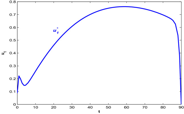
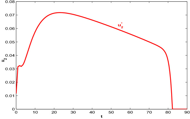
Implementation of both the control policies is beneficial for the proposed optimal system (8). So, we consider the combination of both control policies in the system, i.e., a system where people are maintaining social distancing with time to reduce the virus transmission and they are also taking proper precautionary measures with proper hygiene to stay safe and thereby to move into recovered class directly. Let us consider, $\omega =2\times {10}^{(-4)}$. Figure 13 depict the population trajectories in presence of both the control policies and at $T_f=90$, population becomes (6307329.3, 5.41, 22.49, 32.09, 2.17, 1054.08). The count of recovered individuals reaches its highest level in this case. Also, both the asymptotically exposed and quarantined population decreases than the case when no control is applied. Figure 14 show the paths of optimal control strategies $u_1^{\ast }$ and $u_2^{\ast }$. The control policy on social distancing works with higher intensity throughout the time period and it is true because if people keep maintaining the social distancing, then the virus cannot be transmitted that much. Also, if the susceptible people maintain proper hygiene by using face masks, not touching faces with hands frequently, adopting self-quarantine etc., then also the transmission will be lower. Maintenance of precautionary measures, as denoted by $u_2$, also works its higher intensity for a quite a long time but this intensity is lower than $u_1$.

Fig. 13.

Profiles of populations with both optimal control policies $u_1^{\ast }$ and $u_2^{\ast }$

Fig. 14.

Profiles of optimal controls $u_1^{\ast }$ and $u_2^{\ast }$

In Fig. 15, cost design analysis has been performed in absence and presence of $u_1$ and $u_2$. There is one case when both control policies are applied and the other case contains when there is no control policies is implemented. Optimal cost profiles are shown in figure (15.a) for the cases and trajectory profiles for symptomatically infected individuals are depicted in figure (15.b). In absence of control interventions, cost occurs due to productivity loss by infected only. So, the opportunity loss is higher due to an epidemic outbreak and overall infected population increases in this case. On the other hand, the optimal cost is lower when both control interventions are applied. And as the infected population is lower in this case, it reduces the cost incurred because of opportunity loss.

Fig. 15.

a Cost distribution in presence and absence of control policies. b Profiles of symptomatic infected population under different control policies

Effect of weight constant $w_3$ on optimal control policies

Selection of weight constant on certain control is important. Here we are varying the particular weight constant $w_3$, keeping all other parameters fixed as before, to analyse its impact on the control strategies. It is observed from Fig. 16 and Fig. 17 that if the weight on social distancing increases, then the corresponding associated cost and even the count of symptomatically infected individuals increase.

Fig. 16.

Profiles of cost for various values of $w_3$ along with $w_1=1.5,w_2=2$ and $w_4=50$. The figure on right side is zoomed portion of the left figure. Other parameters are as in Table 2

Fig. 17.

Profiles of symptomatically infective population for various values of $w_3$ along with $w_1=1.5,w_2=2$ and $w_4=50$. Other parameters are as in Table 2

Figure 18 depict that for a smaller value of weight constant $w_3$, the intensity of $u_1$ (which represents social distancing) becomes higher and even works at its highest value but the intensity of $u_2$ (precautionary measures of susceptible individuals) becomes lower with time. So, it is concluded that higher effort for taking precautionary measures and a comparatively lower effort for maintaining social distancing are required to reduce the cost and corresponding count of symptomatically infective individuals when the social distancing has a higher weight. In fact, from Fig. 18a and b, it is observed that when the control intervention denoting social distancing works with the highest intensity, the control policy representing other precautionary measures hardly works. So, we can conclude that if all people maintain the self-isolation, home quarantine strategy or even social distancing properly and strictly, then even a little relaxation in maintaining other precautionary measures can decrease the count of infected individuals and this count is smaller than the rest of the cases.

Fig. 18.

Plots of control a $u_1^{\ast }$ and b $u_2^{\ast }$ for different values of $w_3$ along with $w_1=1.5,w_2=2$ and $w_4=50$. Other parameters are as in Table 2

Conclusion

Coronavirus or COVID-19 first appeared in China in December 2019, but today it has spread all over the world in the form of a pandemic. Reports of the current situation reveal that above 80 lakhs people are infected with the virus worldwide. Though the Governments and medical persons of almost every country are trying to provide protective measures to people, the infection rate is still high enough as the proper antidote for this virus is still unknown. According to the data till 15th June 2020, provided by the dashboard of CSSE at John Hopkins University, United States has the highest confirmed cases with the number 2, 114, 026 [14]. Though according to the official reports, almost 116, 127 people have died in US which is the highest in number among 188 countries or regions. If we consider the current situation in India, then from the reports of CSSE, Worldometers and NIC, India, there are total 343, 091 confirmed Coronavirus cases among which 153, 178 active cases, 9, 900 death cases and 180, 013 recovered cases as reported till 15th June [14–17].

Keeping this pandemic situation in mind, in this work, we have formulated a compartmental SAIRS model of COVID-19. A portion of the susceptible individuals moves into asymptomatically exposed class after getting in touch asymptomatically exposed, symptomatically infected and even hospitalised people. Positivity and boundedness of the system variables prove that the proposed system is well-posed. Feasibility conditions of equilibrium points show that DFE exists for any parametric values whereas the unique endemic equilibrium point exists only when the basic reproduction number $R_c$ lies above unity. Stability analysis of the equilibria has been performed in Sect. 6. Existence of unique endemic equilibrium point for $R_c>1$ concludes that the system undergoes a forward (transcritical) bifurcation around the DFE. If more people move into quarantined class to reduce the virus transmission, then it is obvious that overall infected population decreases with time which is shown in Fig. 6. Also, symptomatically infected population, for increasing quarantine rate of asymptotically exposed people, decreases for increasing value of $\kappa$ (rate of entering of the susceptible individuals to the recovered class). Behavioural changes have been imposed among the susceptible people by keeping social distancing, maintaining proper hygiene, staying at isolation and adopting the self-quarantine method. So, if they take

 precautions at a higher rate and also more people move into quarantine class due to awareness, then the count of symptomatically infected individuals are reduced significantly. As a conclusion, it can be stated that these precautions can be useful to prevent virus transmission at a higher rate.

The corresponding optimal control problem is formulated in the latter part of the work. Control interventions are implemented to reduce the disease burden. Social distancing is one of the prevention strategies that people can adopt to reduce disease transmission. So, we have considered the social distancing of the population as one of the control interventions as it changes with time. Therefore, in the optimal system (8), the disease can be transmitted to $(1-u_1)S$ portion of the susceptible individuals after getting contact with asymptomatically exposed and symptomatically infected individuals. Moreover, the susceptible individuals take different precautionary measures like maintaining proper hygiene, adopting self-quarantine or isolation etc. to prevent the disease transmission. These precautions can be taken as a control policy as it changes with time according to the necessity and disease prevalence. Numerical figures show that the control presenting social distancing $(u_1)$ works with a higher intensity almost after three to four weeks of implementation and continue the intensity level almost throughout the time period. On the other hand, the intensity level of $u_2$ is lesser than $u_1$. The intensity level of $u_2$ first increases within two weeks of implementation and then works with its higher intensity for some time and then decreases. Implementation of either $u_1$ or $u_2$ is useful but applying both $u_1$ and $u_2$ together can reduce asymptomatically exposed people as well as infected population significantly and increase the overall recovered population at a higher rate. Therefore, implementing both the control policies reduce disease transmission in this current pandemic situation.

Appendix

Proof of Theorem 3.1

Right hand side of system (1) is continuous and locally Lipschitzian functions on $\mathbb{C}$ and so there exists an unique solution (S(t), A(t), Q(t), I(t), H(t), R(t)) on $[0,\tau ),$ where $0<\tau \le +\infty$ [40]. First we prove that, $S(t)>0,\forall t\in [0,\tau ).$ If it does not hold, then $\exists t_1\in (0,\tau )$ such that $S(t_1)=0,\dot{S}(t_1)\le 0$ and $S(t)>0,\forall t\in [0,t_1).$ Hence we must have $A(t)\ge 0,\forall t\in [0,t_1).$ If it is not true, then $\exists t_2\in (0,t_1)$ such that $A(t_2)=0,\dot{A}(t_2)<0$ and $A(t)\ge 0,\forall t\in [0,t_2).$ Next we claim $Q(t)\ge 0,\forall t\in [0,t_2).$ Suppose it is not true. Then $\exists t_3\in (0,t_2)$ such that $Q(t_3)=0,\dot{Q}(t_3)<0$ and $Q(t)\ge 0,\forall t\in [0,t_3).$ From third equation of (1), we have

$$\begin{array}{c}\hfill \frac{\mathit{dQ}}{\mathit{dt}}{|}_{t=t_3}=pA(t_3)-(\alpha +\xi +d)Q(t_3)=pA(t_3)\ge 0,\end{array}$$

which is a contradiction to $\dot{Q}(t_3)<0.$ So, $Q(t)\ge 0,\forall t\in [0,t_2).$

Similarly, $I(t)\ge 0,\forall t\in [0,t_2).$

Our next claim is $H(t)\ge 0,\forall t\in [0,t_2).$ Suppose this does not hold, then $\exists t_4\in (0,t_2)$ such that $H(t_4)=0,\dot{H}(t_4)<0$ and $H(t)\ge 0,\forall t\in [0,t_4).$ Now, from the fifth equation of (1):

$$\begin{array}{cc}\hfill \frac{\mathit{dH}}{\mathit{dt}}{|}_{t=t_4}=& \alpha Q(t_4)+\omega I(t_4)-(\varphi +d+{\delta }_3)H(t_4)\hfill \\ \hfill =& \alpha Q(t_4)+\omega I(t_4)\ge 0,\hfill \end{array}$$

which is a contradiction to $\dot{H}(t_4)<0.$ Hence, $H(t)\ge 0,\forall t\in [0,t_2).$

From the second equation of (1), we have

$$\begin{array}{c}\hfill \begin{array}{cc}\hfill \frac{\mathit{dA}}{\mathit{dt}}{|}_{t=t_2}& =({\beta }_{1}A(t_2)+{\beta }_{2}I(t_2)+{\beta }_{3}H(t_2))S(t_2)\hfill \\ \hfill & -(p+\eta +d+{\delta }_1)A(t_2)\hfill \\ \hfill & =({\beta }_{2}I(t_2)+{\beta }_{3}H(t_2))S(t_2)\ge 0\hfill \end{array}\end{array}$$

It is a contradiction to $\dot{A}(t_2)<0.$ So, $A(t)\ge 0,\forall t\in [0,t_1).$ Hence $Q(t)\ge 0,I(t)\ge 0,H(t)\ge 0,\forall t\in [0,t_1).$

Let us claim $R(t)\ge 0,\forall t\in [0,t_1).$ Suppose this does not hold, then $\exists t_5\in (0,t_1)$ such that $R(t_5)=0,\dot{R}(t_5)<0$ and $R(t)\ge 0,\forall t\in [0,t_5).$ From the last equation of (1), we have:

$$\begin{array}{cc}\hfill \frac{\mathit{dR}}{\mathit{dt}}{|}_{t=t_5}=& \kappa S(t_5)+\xi Q(t_5)+\varphi H(t_5)-(d+\psi )R(t_5)\hfill \\ \hfill =& \kappa S(t_5)+\xi Q(t_5)+\varphi H(t_5)>0,\hfill \end{array}$$

which is a contradiction to $\dot{R}(t_5)<0.$ Hence, $R(t)\ge 0,\forall t\in [0,t_1).$

From the first equation of (1), we have

$$\begin{array}{c}\hfill \begin{array}{cc}\hfill \frac{\mathit{dS}}{\mathit{dt}}{|}_{t=t_1}& =\mathrm{\Lambda }-({\beta }_{1}A(t_1)+{\beta }_{2}I(t_1)+{\beta }_{3}H(t_1))S(t_1)\hfill \\ \hfill & -(d+\kappa )S(t_1)+\psi R(t_1)\hfill \\ \hfill & =\mathrm{\Lambda }+\psi R(t_1)>0,\hfill \end{array}\end{array}$$

which is a contradiction to $\dot{S}(t_1)\le 0.$ So, $S(t)>0,\forall t\in [0,\tau ),$ where $0<\tau \le +\infty$. Also, by the previous steps we have $A(t)\ge 0,Q(t)\ge 0,I(t)\ge 0,H(t)\ge 0$ and $R(t)\ge 0,\forall t\in [0,\tau ),$ where $0<\tau \le +\infty .$ Hence it is proved. $\square$

Proof of Theorem 3.2

$$\begin{array}{c}\hfill \begin{array}{cc}\hfill \text{Let},N(t)& =S(t)+A(t)+Q(t)+I(t)+H(t)+R(t)\hfill \\ \hfill \therefore \frac{\mathit{dN}}{\mathit{dt}}& =\mathrm{\Lambda }-d(S+A+Q+I+H+R)\hfill \\ \hfill & -{\delta }_{1}A-{\delta }_{2}I-{\delta }_{3}H\hfill \\ \hfill & =\mathrm{\Lambda }-dN-({\delta }_{1}A+{\delta }_{2}I+{\delta }_{3}H)\hfill \\ \hfill & \le \mathrm{\Lambda }-dN\hfill \\ \hfill & \Rightarrow 0<N(t)\le N(0)e^{-dt}+\frac{\mathrm{\Lambda }}{d}\left(1,-,e^{-dt}\right),\hfill \\ \hfill & \text{where}N(0)=S(0)+A(0)+Q(0)+I(0)\hfill \\ \hfill & +H(0)+R(0).\hfill \end{array}\end{array}$$

As ${\displaystyle t\to \infty ,0<N(t)\le \frac{\mathrm{\Lambda }}{d}.}$ Therefore, all solutions of system (1) enter into the region: ${\displaystyle \mathrm{\Omega }=\left\{(S,A,Q,I,H,R),\in ,{\mathbb{R}}_{+}^6,:,0,<,N,(t),\le ,\frac{\mathrm{\Lambda }}{d}\right\}.}$ $\square$

Proof of Theorem 6.1

Jacobian matrix corresponding to DFE ${\displaystyle E_0=\left(\frac{\mathrm{\Lambda }(d+\psi )}{d(d+\psi +\kappa )},,,0,,,0,,,0,,,0,,,\frac{\mathrm{\Lambda }\kappa }{d(d+\psi +\kappa )}\right)}$ is given as follows:

$$\begin{array}{c}\hfill \overline{J}{|}_{E_0}=\left(\begin{array}{cccccc}-(d+\kappa )& -{\beta }_1{S}_0& 0& -{\beta }_2{S}_0& -{\beta }_3{S}_0& \psi \\ 0& {\beta }_1{S}_0-{\alpha }_0& 0& {\beta }_2{S}_0& {\beta }_3{S}_0& 0\\ 0& p& -{\alpha }_1& 0& 0& 0\\ 0& \eta & 0& -{\alpha }_2& 0& 0\\ 0& 0& \alpha & \omega & -{\alpha }_3& 0\\ \kappa & 0& \xi & 0& \varphi & -(d+\psi )\end{array}\right)\end{array}$$

Two eigenvalues of $\overline{J}{|}_{E_0}$ are roots of the equation: ${\lambda }^2+(2d+\kappa +\psi )\lambda +d(\kappa +d+\psi )=0$ which imply that they are the roots with negative real parts and other four eigenvalues are roots of the following equation: ${\lambda }^4+M_1{\lambda }^3+M_2{\lambda }^2+M_3\lambda +M_4=0,$ where $M_1={\alpha }_0+{\alpha }_1+{\alpha }_2+{\alpha }_3-{\beta }_1{S}_0$, $M_2={\alpha }_0{\alpha }_2+{\alpha }_1{\alpha }_3+({\alpha }_0+{\alpha }_2)({\alpha }_1+{\alpha }_3)-{\beta }_1{S}_0({\alpha }_1+{\alpha }_2+{\alpha }_3)-{\beta }_2{S}_0\eta$, $M_3={\alpha }_0{\alpha }_2({\alpha }_1+{\alpha }_3)+{\alpha }_1{\alpha }_3({\alpha }_0+{\alpha }_2)-{\beta }_1{S}_0\{{\alpha }_1{\alpha }_3+{\alpha }_2({\alpha }_1+{\alpha }_3)\}-{\beta }_2{S}_0\eta ({\alpha }_1+{\alpha }_3)-{\beta }_3{S}_0(p\alpha +\omega \eta )$ and $M_4={\alpha }_0{\alpha }_1{\alpha }_2{\alpha }_3(1-R_c)$. So, $M_4>0$ for $R_c<1$. Therefore the characteristic equation has roots with negative real parts only when $M_1,M_2,M_3>0$ when $R_c<1$. $\square$

Proof of Theorem 6.2

The Jacobian matrix at endemic equilibrium point $E^{\ast }$ is given as:

$$\begin{array}{c}\hfill \overline{J}{|}_{E^{\ast }}=\left(\begin{array}{cccccc}{a}_{11}& a_{12}& 0& a_{14}& a_{15}& a_{16}\\ a_{21}& a_{22}& 0& a_{24}& a_{25}& 0\\ 0& a_{32}& a_{33}& 0& 0& 0\\ 0& a_{42}& 0& a_{44}& 0& 0\\ 0& 0& a_{53}& a_{54}& a_{55}& 0\\ a_{61}& 0& a_{63}& 0& a_{65}& a_{66}\end{array}\right)\end{array}$$

where $a_{11}=-({\beta }_1{A}^{\ast }+{\beta }_2{I}^{\ast }+{\beta }_3{H}^{\ast })-(d+\kappa ),a_{12}=-{\beta }_1{S}^{\ast },a_{14}=-{\beta }_2{S}^{\ast },a_{15}=-{\beta }_3{S}^{\ast },a_{16}=\psi ,a_{21}={\beta }_1{A}^{\ast }+{\beta }_2{I}^{\ast }+{\beta }_3{H}^{\ast },a_{22}={\beta }_1{S}^{\ast }-{\alpha }_0,a_{24}={\beta }_2{S}^{\ast },a_{25}={\beta }_3{S}^{\ast },a_{32}=p,a_{33}=-{\alpha }_1,a_{42}=\eta ,a_{44}=-{\alpha }_2,a_{53}=\alpha ,a_{54}=\omega ,a_{55}=-{\alpha }_3,a_{61}=\kappa ,a_{63}=\xi ,a_{65}=\varphi ,a_{66}=-(d+\psi )$.

Characteristic equation of $\overline{J}{|}_{E^{\ast }}$ is ${\lambda }^6+B_1{\lambda }^5+B_2{\lambda }^4+B_3{\lambda }^3+B_4{\lambda }^2+B_5\lambda +B_6=0,$ where

$$\begin{array}{c}\hfill \begin{array}{cc}\hfill B_1& =-(a_{11}+a_{22}+a_{33}+a_{44}+a_{55}+a_{66})\hfill \\ \hfill & =\frac{({\alpha }_0{\alpha }_2{R}_c^2-{\beta }_1\eta S_0^2)}{\eta S_0{R}_c}{I}^{\ast }+{\alpha }_0+{\alpha }_1\hfill \\ \hfill & +{\alpha }_2+{\alpha }_3+(2d+\kappa +\psi ),\hfill \\ \hfill B_2& =a_{11}(a_{22}+a_{33}+a_{44}+a_{55}+a_{66})-a_{12}{a}_{21}\hfill \\ \hfill & -a_{16}{a}_{61}+a_{22}(a_{33}+a_{44}+a_{55}+a_{66})\hfill \\ \hfill & -a_{24}{a}_{42}+a_{33}(a_{44}+a_{55}+a_{66})\hfill \\ \hfill & +a_{44}(a_{55}+a_{66})+a_{55}{a}_{66},\hfill \\ \hfill B_3& =-a_{11}{a}_{22}(a_{33}+a_{44}+a_{55}+a_{66})+a_{24}{a}_{42}{a}_{11}\hfill \\ \hfill & -a_{11}{a}_{33}(a_{44}+a_{55}+a_{66})-a_{11}{a}_{44}(a_{55}+a_{66})\hfill \\ \hfill & -a_{11}{a}_{55}{a}_{66}+a_{12}{a}_{21}(a_{33}+a_{44}+a_{55}+a_{66})\hfill \\ \hfill & -a_{14}{a}_{42}{a}_{21}+a_{16}{a}_{61}(a_{22}+a_{33}+a_{44}+a_{55})\hfill \\ \hfill & -a_{22}{a}_{33}(a_{44}+a_{55}+a_{66})-a_{22}{a}_{44}(a_{55}+a_{66})\hfill \\ \hfill & -a_{22}{a}_{55}{a}_{66}+a_{24}{a}_{42}(a_{33}+a_{55}+a_{66})-a_{53}{a}_{32}{a}_{25}\hfill \\ \hfill & a_{54}{a}_{42}{a}_{25}-a_{33}{a}_{44}(a_{55}+a_{66})-(a_{33}+a_{44})a_{55}{a}_{66},\hfill \end{array}\end{array}$$

$$\begin{array}{cc}\hfill B_4=& a_{11}{a}_{22}{a}_{33}(a_{44}+a_{55}+a_{66})+a_{11}{a}_{22}{a}_{44}(a_{55}+a_{66})\hfill \\ \hfill & +a_{11}{a}_{22}{a}_{55}{a}_{66}-a_{11}{a}_{24}{a}_{42}(a_{33}+a_{55}+a_{66})\hfill \\ \hfill & a_{11}{a}_{25}(a_{32}{a}_{53}+a_{42}{a}_{54})+a_{11}{a}_{33}{a}_{44}(a_{55}+a_{66})\hfill \\ \hfill & +a_{11}(a_{33}+a_{44})a_{55}{a}_{66}-a_{12}{a}_{21}{a}_{33}(a_{44}+a_{55}+a_{66})\hfill \\ \hfill & -a_{12}{a}_{21}{a}_{44}(a_{55}+a_{66})-a_{12}{a}_{21}{a}_{55}{a}_{66}\hfill \\ \hfill & +a_{14}{a}_{21}{a}_{42}(a_{33}+a_{55}+a_{66})-a_{15}{a}_{21}(a_{33}{a}_{53}+a_{42}{a}_{54})\hfill \\ \hfill & -a_{16}{a}_{21}{a}_{32}{a}_{63}-a_{16}{a}_{22}{a}_{61}(a_{33}+a_{44}+a_{55})\hfill \\ \hfill & +a_{16}{a}_{24}{a}_{42}{a}_{61}-a_{16}{a}_{61}{a}_{33}(a_{44}+a_{55})-a_{16}{a}_{61}{a}_{44}{a}_{55}\hfill \\ \hfill & +a_{22}{a}_{33}{a}_{44}(a_{55}+a_{66})+a_{22}{a}_{55}{a}_{66}(a_{33}+a_{44})\hfill \\ \hfill & -a_{24}{a}_{42}{a}_{33}(a_{55}+a_{66})-a_{24}{a}_{42}{a}_{55}{a}_{66}\hfill \\ \hfill & +a_{25}{a}_{32}{a}_{53}(a_{44}+a_{66})+a_{25}{a}_{42}{a}_{54}(a_{33}+a_{66})\hfill \\ \hfill & +a_{33}{a}_{44}{a}_{55}{a}_{66},\hfill \\ \hfill B_5& =-a_{11}{a}_{22}{a}_{33}{a}_{44}(a_{55}+a_{66})-a_{11}{a}_{22}(a_{33}+a_{44})a_{55}{a}_{66}\hfill \\ \hfill & +a_{11}{a}_{33}{a}_{24}{a}_{42}(a_{55}+a_{66})+a_{11}{a}_{24}{a}_{42}{a}_{55}{a}_{66}\hfill \\ \hfill & -a_{11}{a}_{25}{a}_{32}{a}_{53}(a_{44}+a_{66})-a_{11}{a}_{25}{a}_{42}{a}_{54}(a_{33}\hfill \\ \hfill & +a_{66})-a_{11}{a}_{33}{a}_{44}{a}_{55}{a}_{66}+a_{12}{a}_{21}{a}_{33}{a}_{44}(a_{55}+a_{66})\hfill \\ \hfill & +a_{12}{a}_{21}{a}_{55}{a}_{66}(a_{33}+a_{44})-a_{14}{a}_{21}{a}_{33}{a}_{42}(a_{55}\hfill \\ \hfill & +a_{66})-a_{14}{a}_{21}{a}_{42}{a}_{55}{a}_{66}+a_{15}{a}_{21}{a}_{32}{a}_{53}(a_{44}+a_{66})\hfill \\ \hfill & +a_{15}{a}_{21}{a}_{42}{a}_{54}(a_{33}+a_{66})+a_{16}{a}_{21}{a}_{32}{a}_{63}(a_{44}\hfill \\ \hfill & +a_{55})-a_{16}{a}_{21}{a}_{65}(a_{32}{a}_{53}+a_{42}{a}_{54})\hfill \\ \hfill & +a_{16}{a}_{22}{a}_{33}{a}_{61}(a_{44}+a_{55})+a_{16}{a}_{22}{a}_{44}{a}_{55}{a}_{61}\hfill \\ \hfill & -a_{16}{a}_{24}{a}_{42}{a}_{61}(a_{33}+a_{55})+a_{16}{a}_{25}{a}_{61}(a_{32}{a}_{53}+a_{42}{a}_{54})\hfill \\ \hfill & +a_{16}{a}_{33}{a}_{44}{a}_{55}{a}_{61}-a_{22}{a}_{33}{a}_{44}{a}_{55}{a}_{66}\hfill \\ \hfill & +a_{24}{a}_{33}{a}_{42}{a}_{55}{a}_{66}-a_{25}{a}_{32}{a}_{44}{a}_{53}{a}_{66}-a_{25}{a}_{33}{a}_{42}{a}_{54}{a}_{66},\hfill \\ \hfill B_6& =({\beta }_1{A}^{\ast }+{\beta }_2{I}^{\ast }+{\beta }_3{H}^{\ast })[(d+\psi ){\alpha }_0{\alpha }_1{\alpha }_2{\alpha }_3\hfill \\ \hfill & +p\psi {\alpha }_2(\alpha \varphi +\xi {\alpha }_3)+\kappa \omega \varphi \eta {\alpha }_1]\hfill \\ \hfill & >0,\text{for}{I}^{\ast }>0.\hfill \end{array}$$

Let us consider

$$\begin{array}{c}\hfill \begin{array}{cc}\hfill {\mathrm{\Delta }}_1& =B_1,{\mathrm{\Delta }}_2=\left|\begin{array}{cc}{B}_1& 1\\ B_3& B_2\end{array}\right|,\hfill \\ \hfill {\mathrm{\Delta }}_3& =\left|\begin{array}{ccc}{B}_1& 1& 0\\ B_3& B_2& B_1\\ B_5& B_4& B_3\end{array}\right|,\hfill \\ \hfill {\mathrm{\Delta }}_4& =\left|\begin{array}{cccc}{B}_1& 1& 0& 0\\ B_3& B_2& B_1& 1\\ B_5& B_4& B_3& B_2\\ 0& B_6& B_5& B_4\end{array}\right|,\hfill \\ \hfill {\mathrm{\Delta }}_5& =\left|\begin{array}{ccccc}{B}_1& 1& 0& 0& 0\\ B_3& B_2& B_1& 1& 0\\ B_5& B_4& B_3& B_2& B_1\\ 0& B_6& B_5& B_4& B_3\\ 0& 0& 0& B_6& B_5\end{array}\right|,{\mathrm{\Delta }}_6=Det(\overline{J}{|}_{E^{\ast }})=B_6.\hfill \end{array}\end{array}$$

By Routh-Hurwitz criterion, $E^{\ast }$ is locally asymptomatically stable (LAS) if and only if ${\mathrm{\Delta }}_i>0$ for $i=1,2,3,4,5,6$, i.e., equivalently

• (i)$B_i>0$ for $i=1,6;$
• (ii)${\mathrm{\Delta }}_i>0$ for $i=2,3,4,5$.

$\square$

Proof of Theorem 6.4

Followig Theorem (6.3), we can write system (1) as:

$$\begin{array}{cc}\hfill \frac{\mathit{dX}}{\mathit{dt}}& =F(X,Y),\hfill \\ \hfill \frac{\mathit{dY}}{\mathit{dt}}& =G(X,Y),G(X,O)=O,\hfill \\ \hfill \text{where}F(X,Y)& =\left(\begin{array}{c}\mathrm{\Lambda }-({\beta }_{1}A+{\beta }_{2}I+{\beta }_{3}H)S+\psi R-(d+\kappa )S\\ \kappa S+\xi Q+\varphi H-(d+\psi )R\end{array}\right)\hfill \\ \hfill \text{and}G(X,Y)& =\left(\begin{array}{c}({\beta }_{1}A+{\beta }_{2}I+{\beta }_{3}H)S-{\alpha }_{0}A\\ pA-{\alpha }_{1}Q\\ \eta A-{\alpha }_{2}I\\ \alpha Q+\omega I-{\alpha }_{3}H\end{array}\right)\hfill \end{array}$$

Here $G(X,O)=O$ taking $X={(S,R)}^T$ and $Y={(A,Q,I,H)}^T$. The DFE of system (1) is $U_0=E_0={(X_0,O)}^T$ with ${\displaystyle X_0\equiv (S_0,R_0)=\left(\frac{\mathrm{\Lambda }(d+\psi )}{d(d+\psi +\kappa )},,,\frac{\mathrm{\Lambda }\kappa }{d(d+\psi +\kappa )}\right)}$. Clearly $X_0$ is globally asymptotically stable for ${\displaystyle \frac{\mathit{dX}}{\mathit{dt}}=F(X,O)}$ as $X\to {(S_0,R_0)}^T$ whenever $t\to \infty$. Further we have

$$\begin{array}{c}\hfill \begin{array}{cc}\hfill G(X,Y)& =D_{Y}G(X_0,O)Y-\overline{G}(X,Y)\hfill \\ \hfill & =\left(\begin{array}{cccc}{\beta }_1{S}_0-{\alpha }_0& 0& {\beta }_2{S}_0& {\beta }_3{S}_0\\ p& -{\alpha }_1& 0& 0\\ \eta & 0& -{\alpha }_2& 0\\ 0& \alpha & \omega & -{\alpha }_3\end{array}\right).\left(\begin{array}{c}A\\ Q\\ I\\ H\end{array}\right)\hfill \\ \hfill & -\left(\begin{array}{c}(S_0-S)({\beta }_{1}A+{\beta }_{2}I+{\beta }_{3}H)\\ 0\\ 0\\ 0\end{array}\right)\hfill \end{array}\end{array}$$

Here $B(X,Y)=D_{Y}G(X_0,O)$ is a stable matrix when local stability criterion of $E_0$ holds along with $R_c<1$ and the off-diagonal elements are non-negative also implying B(X, Y) is a M-matrix. Moreover, $\overline{G}(X,Y)\ge O$ when $S\le S_0\le \frac{\mathrm{\Lambda }}{d}$. Hence the assumptions (H1) and (H2) are satisfied and by Theorem (6.3), DFE $E_0$ of system (1) is globally asymptotically stable when $S\le S_0$ for $R_c<1$. $\square$

Proof of Theorem 6.5

Consider a Lyapunov function V(t) as:

$$\begin{array}{c}\hfill \begin{array}{cc}\hfill V(t)& =\left(S,-,S^{\ast },-,S^{\ast },l,n,\frac{S}{S^{\ast }}\right)+m_1\left(A,-,A^{\ast },-,A^{\ast },l,n,\frac{A}{A^{\ast }}\right)\hfill \\ \hfill & +m_2\left(Q,-,Q^{\ast },-,Q^{\ast },l,n,\frac{Q}{Q^{\ast }}\right)\hfill \\ \hfill & +m_3\left(I,-,I^{\ast },-,I^{\ast },l,n,\frac{I}{I^{\ast }}\right)+m_4\left(H,-,H^{\ast },-,H^{\ast },l,n,\frac{H}{H^{\ast }}\right)\hfill \\ \hfill & +m_5\left(R,-,R^{\ast },-,R^{\ast },l,n,\frac{R}{R^{\ast }}\right)\hfill \end{array}\end{array}$$

Time derivative of V along the solutions of system (1) is given by

$$\begin{array}{cc}\hfill \frac{\mathit{dV}}{\mathit{dt}}& =\left(1,-,\frac{S^{\ast }}{S}\right)[\mathrm{\Lambda }-({\beta }_{1}A+{\beta }_{2}I+{\beta }_{3}H)S\hfill \\ \hfill & +\psi R-(d+\kappa )S]\hfill \\ \hfill & +m_1\left(1,-,\frac{A^{\ast }}{A}\right)[({\beta }_{1}A+{\beta }_{2}I+{\beta }_{3}H)S-{\alpha }_{0}A]\hfill \\ \hfill & +m_2\left(1,-,\frac{Q^{\ast }}{Q}\right)[pA-{\alpha }_{1}Q]\hfill \\ \hfill & +m_3\left(1,-,\frac{I^{\ast }}{I}\right)[\eta A-{\alpha }_{2}I]\hfill \\ \hfill & +m_4\left(1,-,\frac{H^{\ast }}{H}\right)[\alpha Q+\omega I-{\alpha }_{3}H]\hfill \\ \hfill & +m_5\left(1,-,\frac{R^{\ast }}{R}\right)[\kappa S+\xi Q+\varphi H-(d+\psi )R]\hfill \\ \hfill & =\left(1,-,\frac{S^{\ast }}{S}\right)[{\beta }_1(A^{\ast }{S}^{\ast }-SA)+{\beta }_2(I^{\ast }{S}^{\ast }-SI)\hfill \\ \hfill & +{\beta }_3(H^{\ast }{S}^{\ast }-SH)+\psi (R-R^{\ast })\hfill \\ \hfill & -(d+\kappa )(S-S^{\ast })]+m_1\left(1,-,\frac{A^{\ast }}{A}\right)\hfill \\ \hfill & [-{\beta }_1(A^{\ast }{S}^{\ast }-SA)\hfill \\ \hfill & -{\beta }_2(I^{\ast }{S}^{\ast }-SI)-{\beta }_3(H^{\ast }{S}^{\ast }-SH)\hfill \\ \hfill & -{\alpha }_0(A-A^{\ast })]+m_2\left(1,-,\frac{Q^{\ast }}{Q}\right)\hfill \\ \hfill & [p(A-A^{\ast })-{\alpha }_1(Q-Q^{\ast })]\hfill \\ \hfill & +m_3\left(1,-,\frac{I^{\ast }}{I}\right)[\eta (A-A^{\ast })\hfill \\ \hfill & -{\alpha }_2(I-I^{\ast })]+m_4\left(1,-,\frac{H^{\ast }}{H}\right)[\alpha (Q-Q^{\ast })\hfill \\ \hfill & +\omega (I-I^{\ast })-{\alpha }_3(H-H^{\ast })]\hfill \\ \hfill & +m_5\left(1,-,\frac{R^{\ast }}{R}\right)[\kappa (S-S^{\ast })\hfill \\ \hfill & +\xi (Q-Q^{\ast })+\varphi (H-H^{\ast })-(d+\psi )(R-R^{\ast })]\hfill \end{array}$$

Let, $\frac{S}{S^{\ast }}=x,\frac{A}{A^{\ast }}=y,\frac{Q}{Q^{\ast }}=z,\frac{I}{I^{\ast }}=u,\frac{H}{H^{\ast }}=v$ and $\frac{R}{R^{\ast }}=l.$ So, we have

$$\begin{array}{cc}\hfill \frac{\mathit{dV}}{\mathit{dt}}& =\left(1,-,\frac{1}{x}\right)[-S^{\ast }({\beta }_1{A}^{\ast }+{\beta }_2{I}^{\ast }+{\beta }_3{H}^{\ast }+d+\kappa )(x-1)\hfill \\ \hfill & -{\beta }_{1}S{A}^{\ast }(y-1)-{\beta }_{2}S{I}^{\ast }(u-1)\hfill \\ \hfill & -{\beta }_{3}S{H}^{\ast }(v-1)+\psi R^{\ast }(l-1)]+m_1\left(1,-,\frac{1}{y}\right)\hfill \\ \hfill & [S^{\ast }({\beta }_1{A}^{\ast }+{\beta }_2{I}^{\ast }+{\beta }_3{H}^{\ast })(x-1)+{\beta }_{1}S{A}^{\ast }(y-1)\hfill \\ \hfill & +{\beta }_{2}S{I}^{\ast }(u-1)+{\beta }_{3}S{H}^{\ast }(v-1)-{\alpha }_0{A}^{\ast }(y-1)]\hfill \\ \hfill & +m_2\left(1,-,\frac{1}{z}\right)[p{A}^{\ast }(y-1)-{\alpha }_1{Q}^{\ast }(z-1)]\hfill \\ \hfill & +m_3\left(1,-,\frac{1}{u}\right)[\eta A^{\ast }(y-1)-{\alpha }_{2}I\ast (u-1)]\hfill \\ \hfill & +m_4\left(1,-,\frac{1}{v}\right)[\alpha Q^{\ast }(z-1)+\omega I^{\ast }(u-1)\hfill \\ \hfill & -{\alpha }_3{H}^{\ast }(v-1)]+m_5\left(1,-,\frac{1}{l}\right)[\kappa S^{\ast }(x-1)\hfill \\ \hfill & +\xi Q^{\ast }(z-1)+\varphi H^{\ast }(v-1)-(d+\psi )R^{\ast }(l-1)]\hfill \end{array}$$

Now steady state of system (1) at $E^{\ast }$ gives ${\displaystyle \mathrm{\Lambda }-({\beta }_1{A}^{\ast }+{\beta }_2{I}^{\ast }+{\beta }_3{H}^{\ast })S^{\ast }+\psi R^{\ast }=(d+\kappa )S^{\ast },({\beta }_1{A}^{\ast }+{\beta }_2{I}^{\ast }+{\beta }_3{H}^{\ast })S={\alpha }_0{A}^{\ast },p{A}^{\ast }={\alpha }_1{Q}^{\ast },\eta A^{\ast }={\alpha }_2{I}^{\ast },\alpha Q^{\ast }+\omega I^{\ast }={\alpha }_3{H}^{\ast },\kappa S^{\ast }+\xi Q^{\ast }+\varphi H^{\ast }=(d+\psi )R^{\ast }}$. Also, we take $m_1,m_5=1$. So, we have

$$\begin{array}{cc}\hfill \frac{\mathit{dV}}{\mathit{dt}}=& S^{\ast }({\beta }_1{A}^{\ast }+{\beta }_2{I}^{\ast }+{\beta }_3{H}^{\ast }+d+\kappa )\left(2,-,x,-,\frac{1}{x}\right)\hfill \\ \hfill & +{\alpha }_0{A}^{\ast }\left(2,-,y,-,\frac{1}{y}\right)\hfill \\ \hfill & +m_2{\alpha }_1{Q}^{\ast }\left(2,-,z,-,\frac{1}{z}\right)+m_3{\alpha }_2{I}^{\ast }\left(2,-,u,-,\frac{1}{u}\right)\hfill \\ \hfill & +m_4{\alpha }_3{H}^{\ast }\left(2,-,v,-,\frac{1}{v}\right)\hfill \\ \hfill & +m_5(d+\psi )R^{\ast }\left(2,-,l,-,\frac{1}{l}\right)\hfill \\ \hfill & -{\beta }_{1}S{A}^{\ast }\left(1,-,\frac{y}{x},+,\frac{1}{x},-,\frac{1}{y}\right)-{\beta }_{2}S{I}^{\ast }\left(\frac{u}{y},-,\frac{u}{x},+,\frac{1}{x},-,\frac{1}{y}\right)\hfill \\ \hfill & -{\beta }_{3}S{H}^{\ast }\left(\frac{v}{y},-,\frac{v}{x},+,\frac{1}{x},-,\frac{1}{y}\right)+\psi R^{\ast }\left(l,-,1,-,\frac{l}{x},+,\frac{1}{x}\right)\hfill \\ \hfill & +m_{2}p{A}^{\ast }\left(y,-,1,-,\frac{y}{z},+,\frac{1}{z}\right)\hfill \\ \hfill & +({\beta }_1{A}^{\ast }+{\beta }_2{I}^{\ast }+{\beta }_3{H}^{\ast })S^{\ast }\left(x,-,1,-,\frac{x}{y},+,\frac{1}{y}\right)\hfill \\ \hfill & +m_3\eta A^{\ast }\left(y,-,1,-,\frac{y}{u},+,\frac{1}{u}\right)\hfill \\ \hfill & +m_4\alpha Q^{\ast }\left(z,-,1,-,\frac{z}{v},+,\frac{1}{v}\right)\hfill \\ \hfill & +m_4\omega I^{\ast }\left(u,-,1,-,\frac{u}{v},+,\frac{1}{v}\right)\hfill \\ \hfill & +m_5\xi Q^{\ast }\left(z,-,1,-,\frac{z}{l},+,\frac{1}{l}\right)\hfill \\ \hfill & +m_5\kappa S^{\ast }\left(x,-,1,-,\frac{x}{l},+,\frac{1}{l}\right)+m_5\varphi H^{\ast }\left(v,-,1,-,\frac{v}{l},+,\frac{1}{l}\right)\hfill \\ \hfill & ={\alpha }_0{A}^{\ast }\left(3,-,\frac{1}{x},-,\frac{x}{y},-,y\right)+(d+\kappa )\left(2,-,x,-,\frac{1}{x}\right)\hfill \\ \hfill & +m_2{\alpha }_1{Q}^{\ast }\left(1,+,y,-,z,-,\frac{y}{z}\right)\hfill \\ \hfill & +m_3{\alpha }_2{I}^{\ast }\left(1,+,y,-,u,-,\frac{y}{u}\right)+m_4\alpha Q^{\ast }\left(1,+,z,-,v,-,\frac{z}{v}\right)\hfill \\ \hfill & +m_4\omega I^{\ast }\left(1,+,u,-,v,-,\frac{u}{v}\right)\hfill \\ \hfill & +d{R}^{\ast }\left(2,-,l,-,\frac{1}{l}\right)+{\beta }_{1}S{A}^{\ast }\hfill \\ \hfill & \left(\frac{1}{y},+,\frac{y}{x},-,1,-,\frac{1}{x}\right)\hfill \\ \hfill & +{\beta }_{2}S{I}^{\ast }\left(\frac{1}{y},+,\frac{u}{x},-,\frac{1}{x},-,\frac{u}{y}\right)\hfill \\ \hfill & +{\beta }_{3}S{H}^{\ast }\left(\frac{1}{y},+,\frac{v}{x},-,\frac{1}{x},-,\frac{v}{y}\right)+\psi R^{\ast }\left(1,+,\frac{1}{x},-,\frac{l}{x},-,\frac{1}{l}\right)\hfill \\ \hfill & +\xi Q^{\ast }\left(z,-,1,-,\frac{z}{l},+,\frac{1}{l}\right)\hfill \\ \hfill & +\kappa S^{\ast }\left(x,-,1,-,\frac{x}{l},+,\frac{1}{l}\right)+\varphi H^{\ast }\left(v,-,1,-,\frac{v}{l},+,\frac{1}{l}\right)\hfill \end{array}$$

Let us consider $m_4=\frac{\varphi +{\beta }_3{S}^{\ast }}{\alpha 3},m_2=\frac{\xi +m_4\alpha }{{\alpha }_1}$ and $m_3=\frac{{\beta }_2{S}^{\ast }+m_4\omega }{{\alpha }_2}.$ So, ${\displaystyle \frac{\mathit{dV}}{\mathit{dt}}\le 0}$ in the region $\mathrm{\Phi }$ provided following conditions are satisfied,

${\displaystyle (i)\psi S^{\ast }{R}^{\ast }<2{\alpha }_0{S}^{\ast }{A}^{\ast }}$ and ${\displaystyle (ii)p{m}_2{\alpha }_2+\eta m_3{\alpha }_2+{\beta }_1{\alpha }_2{S}^{\ast }<{\alpha }_0{\alpha }_2}$.

Moreover, ${\displaystyle \frac{\mathit{dV}}{\mathit{dt}}{|}_{E^{\ast }}=0}$. So, by Lyapunov LaSalle’s theorem [41], $E^{\ast }$ is GAS in the interior of $\mathrm{\Phi }$ subject to the stated parametric conditions. $\square$

Existence of optimal control functions

Now we derive the conditions for existence of optimal control interventions which also minimize the cost function J in a finite time period.

Proof of Theorem 9.1

The optimal control variables, when exist, satisfy the following conditions:

• (i)Solutions of system (8) with control variables $u_1$ and $u_2$ in $\mathrm{\Pi }\ne \varphi$.
• (ii)The mentioned set $\mathrm{\Pi }$ is closed, convex and the state system is represented with linear function of control variables where coefficients depend on time and also on state variables.
• (iii)
  Integrand of (7): L is convex on $\mathrm{\Pi }$ and $L(S,A,Q,I,H,R,u_1,u_2)\ge h(u_1,u_2)$ where $h(u_1,u_2)$ is continuous and $||(u_1,u_2){||}^{-1}h(u_1,u_2)\to \infty$ when $||(u_1,u_2)||\to \infty$; ||.|| represents the $L^2(0,T_f)$ norm. From (8), the total population $N=S+A+Q+I+H+R.$

  $$\begin{array}{c}\hfill \begin{array}{cc}\hfill \text{So,}\frac{\mathit{dN}}{\mathit{dt}}& =\mathrm{\Lambda }-dN-{\delta }_{1}A-{\delta }_{2}I-{\delta }_{3}H\le \mathrm{\Lambda }-dN\hfill \\ \hfill & \Rightarrow 0<N(t)\le N(0)e^{-dt}+\frac{\mathrm{\Lambda }}{d}\left(1,-,e^{-dt}\right),\hfill \end{array}\end{array}$$

  where $N(0)=S(0)+A(0)+Q(0)+I(0)+H(0)+R(0)$. As ${\displaystyle t\to \infty ,0<N(t)\le \frac{\mathrm{\Lambda }}{d}.}$ For each of the control variable in $\mathrm{\Pi }$, solution of (8) is bounded and right hand side functions are locally Lipschitzian too. $Picard-Lindel\ddot{o}f$ theorem shows that condition (i) is satisfied [42]. The control set $\mathrm{\Pi }$ is closed and convex by definition. Again all the equations of system (8) are written as linear equations in $u_1$ and $u_2$ where state variables depend on coefficients and hence condition (ii) is satisfied also. Moreover, the quadratic nature of all control variables guarantee the convex property of integrand $L(S,A,Q,I,H,R,u_1,u_2)$.

  $$\begin{array}{c}\hfill \begin{array}{cc}& \text{Also,}L(S,A,Q,I,H,R,u_1,u_2)\hfill \\ \hfill & =w_{1}A+w_{2}I+w_3{u}_1^2+w_4{u}_2^2\hfill \\ \hfill & \ge w_3{u}_1^2+w_4{u}_2^2\hfill \end{array}\end{array}$$

  Let, $\overline{w}=min(w_3,w_4)>0$ and $k(u_1,u_2)=\overline{w}(u_1^2+u_2^2).$ Then $L(S,A,Q,I,H,R,u_1,u_2)\ge k(u_1,u_2).$ Here k is continuous and $||(u_1,u_2){||}^{-1}k(u_1,u_2)\to \infty$ whenever $||(u_1,u_2)||\to \infty .$ Hence, condition (iii) is also satisfied. So, it is concluded that there exist control variables $u_1^{\ast }$ and $u_2^{\ast }$ with the condition $J[u_1^{\ast },u_2^{\ast }]=min[J[u_1,u_2]]$ [38, 43].

Characterization of optimal control functions

By Pontryagin’s Maximum Principle, we have derived here the necessary conditions for optimal control functions for system (7)-(8) [43–47]. Let us define the Hamiltonian function as:

$$\begin{array}{c}\hfill \begin{array}{cc}& \overline{H}\left(S,,,A,,,Q,,,I,,,H,,,R,,,u_1,,,u_2,,,\lambda \right)\hfill \\ \hfill & =L(S,A,Q,I,H,R,u_1,u_2)+{\lambda }_1\frac{\mathit{dS}}{\mathit{dt}}+{\lambda }_2\frac{\mathit{dA}}{\mathit{dt}}+{\lambda }_3\frac{\mathit{dQ}}{\mathit{dt}}\hfill \\ \hfill & +{\lambda }_4\frac{\mathit{dI}}{\mathit{dt}}+{\lambda }_5\frac{\mathit{dH}}{\mathit{dt}}+{\lambda }_6\frac{\mathit{dR}}{\mathit{dt}}\hfill \\ \hfill & \text{So},\overline{H}\hfill \\ \hfill & =w_{1}A+w_{2}I+w_3{u}_1^2+w_4{u}_2^2+{\lambda }_1[\mathrm{\Lambda }-(1-u_1(t))({\beta }_{1}A\hfill \\ \hfill & +{\beta }_{2}I)S-{\beta }_{3}HS-dS+\psi R\hfill \\ \hfill & -u_2(t)S]+{\lambda }_2[(1-u_1(t))({\beta }_{1}A+{\beta }_{2}I)S+{\beta }_{3}HS-{\alpha }_{0}A]\hfill \\ \hfill & +{\lambda }_3[pA-{\alpha }_{1}Q]+{\lambda }_4[\eta A-{\alpha }_{2}I]\hfill \\ \hfill & +{\lambda }_5[\alpha Q+\omega I-{\alpha }_{3}H]+{\lambda }_6[\xi Q+u_2(t)S\hfill \\ \hfill & +\varphi H-(d+\psi )R]\hfill \end{array}\end{array}$$ 11

Here $\lambda =\left({\lambda }_1,,,{\lambda }_2,,,{\lambda }_3,,,{\lambda }_4,,,{\lambda }_5,,,{\lambda }_6\right)$ are the adjoint variables. We get minimized Hamiltonian by Pontryagin’s Maximum Principle to minimize the cost functional. Pontryagin’s Maximum Principle mainly adjoin the cost functional with the state equations by introducing adjoint variables.

Proof of Theorem 9.2

Let $u_1^{\ast }$ and $u_2^{\ast }$ be optimal control variables and $S^{\ast },A^{\ast },Q^{\ast },I^{\ast },H^{\ast },R^{\ast }$ are corresponding optimal state variables of the control system (8) which minimize the cost functional (7). So, by Pontryagin’s Maximum Principle, there exist adjoint variables ${\lambda }_1,{\lambda }_2,{\lambda }_3,{\lambda }_4,{\lambda }_5,{\lambda }_6$ which satisfy the following canonical equations:

$$\begin{array}{c}\hfill \begin{array}{cc}& \frac{d{\lambda }_1}{\mathit{dt}}=-\frac{\partial \overline{H}}{\partial S},\frac{d{\lambda }_2}{\mathit{dt}}=-\frac{\partial \overline{H}}{\partial A},\frac{d{\lambda }_3}{\mathit{dt}}=-\frac{\partial \overline{H}}{\partial Q},\hfill \\ \hfill & \frac{d{\lambda }_4}{\mathit{dt}}=-\frac{\partial \overline{H}}{\partial I},\frac{d{\lambda }_5}{\mathit{dt}}=-\frac{\partial \overline{H}}{\partial H},\hfill \\ \hfill & \frac{d{\lambda }_6}{\mathit{dt}}=-\frac{\partial \overline{H}}{\partial R}.\hfill \end{array}\end{array}$$

So, we have

$$\begin{array}{cc}\hfill \frac{d{\lambda }_1}{\mathit{dt}}& ={\lambda }_1[({\beta }_{1}A+{\beta }_{2}I)(1-u_1)+{\beta }_{3}H+u_2+d]\hfill \\ \hfill & -{\lambda }_2[({\beta }_{1}A+{\beta }_{2}I)(1-u_1)+{\beta }_{3}H]-{\lambda }_6(u_2)\hfill \\ \hfill \frac{d{\lambda }_2}{\mathit{dt}}& =-w_1+{\lambda }_1[(1-u_1){\beta }_{1}S]\hfill \\ \hfill & -{\lambda }_2[(1-u_1){\beta }_{1}S-{\alpha }_0]-{\lambda }_3(p)-{\lambda }_4(\eta )\hfill \\ \hfill \frac{d{\lambda }_3}{\mathit{dt}}& ={\lambda }_3({\alpha }_1)-{\lambda }_5(\alpha )-{\lambda }_6(\xi )\hfill \\ \hfill \frac{d{\lambda }_4}{\mathit{dt}}& =-w_2+{\lambda }_1[(1-u_1){\beta }_{2}S]-{\lambda }_2[(1-u_1){\beta }_{2}S]\hfill \\ \hfill & +{\lambda }_4({\alpha }_2)-{\lambda }_5(\omega )\hfill \\ \hfill \frac{d{\lambda }_5}{\mathit{dt}}& ={\lambda }_1({\beta }_{3}S)-{\lambda }_2({\beta }_{3}S)+{\lambda }_5({\alpha }_3)-{\lambda }_6(\varphi )\hfill \\ \hfill \frac{d{\lambda }_6}{\mathit{dt}}& =-{\lambda }_1(\psi )+{\lambda }_6(d+\psi )\hfill \end{array}$$ 12

with the transversality conditions ${\lambda }_i(T_f)=0$, for $i=1,2,3,4,5,6.$

$$\begin{array}{c}\hfill \text{From optimality conditions}:\frac{\partial \overline{H}}{\partial u_1}{|}_{u_1=u_1^{\ast }}=0\text{and}\frac{\partial \overline{H}}{\partial u_2}{|}_{u_2=u_2^{\ast }}=0.\end{array}$$

So, ${\displaystyle u_1^{\ast }=\frac{S^{\ast }({\beta }_1{A}^{\ast }+{\beta }_2{I}^{\ast })}{2w_3}\left({\lambda }_2,-,{\lambda }_1\right),u_2^{\ast }=\frac{S^{\ast }}{2w_4}\left({\lambda }_1,-,{\lambda }_6\right)}$.

Now from these findings along with the characteristics of control set $\mathrm{\Pi },$ we have

$$\begin{array}{c}\hfill \begin{array}{cc}\hfill u_1^{\ast }& =\left\{\begin{array}{cc}0,\hfill & \text{if}\frac{S^{\ast }({\beta }_1{A}^{\ast }+{\beta }_2{I}^{\ast })}{2w_3}\left({\lambda }_2,-,{\lambda }_1\right)<0\hfill \\ \hfill \\ \frac{S^{\ast }({\beta }_1{A}^{\ast }+{\beta }_2{I}^{\ast })}{2w_3}\left({\lambda }_2,-,{\lambda }_1\right),\hfill & \text{if}0\le \frac{S^{\ast }({\beta }_1{A}^{\ast }+{\beta }_2{I}^{\ast })}{2w_3}\left({\lambda }_2,-,{\lambda }_1\right)\le 1\hfill \\ \hfill \\ 1,\hfill & \text{if}\frac{S^{\ast }({\beta }_1{A}^{\ast }+{\beta }_2{I}^{\ast })}{2w_3}\left({\lambda }_2,-,{\lambda }_1\right)>1\hfill \end{array}\right)\hfill \end{array}\end{array}$$

$$\begin{array}{c}\hfill \begin{array}{cc}\hfill u_2^{\ast }& =\left\{\begin{array}{cc}0,\hfill & \text{if}\frac{S^{\ast }}{2w_4}\left({\lambda }_1,-,{\lambda }_6\right)<0\hfill \\ \hfill \\ \frac{S^{\ast }}{2w_4}\left({\lambda }_1,-,{\lambda }_6\right),\hfill & \text{if}0\le \frac{S^{\ast }}{2w_4}\left({\lambda }_1,-,{\lambda }_6\right)\le 1\hfill \\ \hfill \\ 1,\hfill & \text{if}\frac{S^{\ast }}{2w_4}\left({\lambda }_1,-,{\lambda }_6\right)>1\hfill \end{array}\right)\hfill \end{array}\end{array}$$

which is equivalent as (10). $\square$

Optimal system

We state the optimal system with optimal control variables $u_1^{\ast }$ and $u_2^{\ast }$ below. The optimal system with minimized Hamiltonian ${\overline{H}}^{\ast }$ at $(S^{\ast },A^{\ast },Q^{\ast },I^{\ast },H^{\ast },R^{\ast },{\lambda }_1,{\lambda }_2,{\lambda }_3,{\lambda }_4,{\lambda }_5,{\lambda }_6)$ is as follows:

$$\begin{array}{cc}\hfill \frac{d{S}^{\ast }}{\mathit{dt}}& =\mathrm{\Lambda }-(1-u_1^{\ast })({\beta }_1{A}^{\ast }+{\beta }_2{I}^{\ast })S^{\ast }\hfill \\ \hfill & -{\beta }_3{H}^{\ast }{S}^{\ast }-d{S}^{\ast }+\psi R^{\ast }-u_2^{\ast }{S}^{\ast },\hfill \\ \hfill \frac{d{A}^{\ast }}{\mathit{dt}}& =(1-u_1^{\ast })({\beta }_1{A}^{\ast }+{\beta }_2{I}^{\ast })S^{\ast }+{\beta }_3{H}^{\ast }{S}^{\ast }-{\alpha }_0{A}^{\ast },\hfill \\ \hfill \frac{d{Q}^{\ast }}{\mathit{dt}}& =p{A}^{\ast }-{\alpha }_1{Q}^{\ast },\hfill \\ \hfill \frac{d{I}^{\ast }}{\mathit{dt}}& =\eta A^{\ast }-{\alpha }_2{I}^{\ast },\hfill \\ \hfill \frac{d{H}^{\ast }}{\mathit{dt}}& =\alpha Q^{\ast }+\omega I^{\ast }-{\alpha }_3{H}^{\ast },\hfill \\ \hfill \frac{d{R}^{\ast }}{\mathit{dt}}& =u_2^{\ast }{S}^{\ast }+\xi Q^{\ast }+\varphi H^{\ast }-(d+\psi )R^{\ast },\hfill \end{array}$$ 13

with initial conditions: $S^{\ast }(0)>0,A^{\ast }(0)\ge 0,Q^{\ast }(0)\ge 0,I^{\ast }(0)\ge 0,H^{\ast }\ge 0$ and $R^{\ast }\ge 0$. The corresponding adjoint system is given as:

$$\begin{array}{c}\hfill \begin{array}{cc}\hfill \frac{d{\lambda }_1}{\mathit{dt}}& ={\lambda }_1[({\beta }_1{A}^{\ast }+{\beta }_2{I}^{\ast })(1-u_1^{\ast })+{\beta }_3{H}^{\ast }+u_2^{\ast }+d]\hfill \\ \hfill & -{\lambda }_2[({\beta }_1{A}^{\ast }+{\beta }_2{I}^{\ast })(1-u_1^{\ast })+{\beta }_3{H}^{\ast }]-{\lambda }_6(u_2^{\ast })\hfill \\ \hfill \frac{d{\lambda }_2}{\mathit{dt}}& =-w_1+{\lambda }_1[(1-u_1^{\ast }){\beta }_1{S}^{\ast }]\hfill \\ \hfill & -{\lambda }_2[(1-u_1^{\ast }){\beta }_1{S}^{\ast }-{\alpha }_0]-{\lambda }_3(p)-{\lambda }_4(\eta )\hfill \\ \hfill \frac{d{\lambda }_3}{\mathit{dt}}& ={\lambda }_3({\alpha }_1)-{\lambda }_5(\alpha )-{\lambda }_6(\xi )\hfill \\ \hfill \frac{d{\lambda }_4}{\mathit{dt}}& =-w_2+{\lambda }_1[(1-u_1^{\ast }){\beta }_2{S}^{\ast }]-{\lambda }_2[(1-u_1^{\ast }){\beta }_2{S}^{\ast }]\hfill \\ \hfill & +{\lambda }_4({\alpha }_2)-{\lambda }_5(\omega )\hfill \\ \hfill \frac{d{\lambda }_5}{\mathit{dt}}& ={\lambda }_1({\beta }_3{S}^{\ast })-{\lambda }_2({\beta }_3{S}^{\ast })+{\lambda }_5({\alpha }_3)-{\lambda }_6(\varphi )\hfill \\ \hfill \frac{d{\lambda }_6}{\mathit{dt}}& =-{\lambda }_1(\psi )+{\lambda }_6(d+\psi ),\hfill \end{array}\end{array}$$ 14

with transversality conditions ${\lambda }_i(T_f)=0$, for $i=1,2,\dots ,6$ and $u_1^{\ast }$ and $u_2^{\ast }$ are same as in (10).

Data Availability

The data used in this work have been obtained from official sources cited in the references [14–17]. The data that support the findings of this study are available from the corresponding author upon reasonable request.

Conflict of Interest

The authors declare that they have no conflict of interest.

References

- 1.Chen N, Zhou M, Dong X, Qu J, Gong F, Han Y, Qiu Y, Wang J, Liu Y, Wei Y, Xia J, Yu T, Zhang X, Zhang L. Epidemiological and clinical characteristics of 99 cases of 2019 novel coronavirus pneumonia in Wuhan, China: a descriptive study. Lancet. 2020;395(10223):507–513. doi: 10.1016/S0140-6736(20)30211-7. [DOI] [PMC free article] [PubMed] [Google Scholar]
- 2.Li R, Pei S, Chen B, Song Y, Zhang T, Yang W, Shaman J. Substantial undocumented infection facilitates the rapid dissemination of novel coronavirus (SARS-CoV2) Science. 2020;368(6490):489–493. doi: 10.1126/science.abb3221. [DOI] [PMC free article] [PubMed] [Google Scholar]
- 3.Chen W, Horby PW, Hayden FG, Gao GF. A novel coronavirus outbreak of global health concern. The Lancet. 2020;395(10223):470–473. doi: 10.1016/S0140-6736(20)30211-7. [DOI] [PMC free article] [PubMed] [Google Scholar]
- 4.Juan D (2020) Wuhan wet market closes amid pneumonia outbreak. https://www.chinadaily.com.cn/a/202001/01/WS5e0c6a49a310cf3e35581e30.html
- 5.Coronaviridae Study Group of the International Committee on Taxonomy of Viruses The species Severe acute respiratory syndrome-related coronavirus: classifying 2019-nCoV and naming it SARS-CoV-2. Nat Microbiol. 2020;5(4):536–544. doi: 10.1038/s41564-020-0695-z. [DOI] [PMC free article] [PubMed] [Google Scholar]
- 6.Richman DD, Whitley RJ, Hayden FG. Clinical virology. Hoboken: Wiley; 2016. [Google Scholar]
- 7.Gaythorpe K, Imai N, Cuomo-Dannenburg G, Baguelin M, Bhatia S, Boonyasiri A, Cori A, Cucunub Z, Dighe A, Dorigatti I, FitzJohn R, Fu H, Laydon D, Nedjati-Gilani G, Okell L, Riley S, Thompson H, van Elsland S, Wang H, Wang Y, Whittaker C, Xi X, Donnelly CA, Ghani A (2020) Report 8: symptom progression of COVID-19. https://www.imperial.ac.uk/mrc-global-infectious-disease-analysis/covid-19/report-8-symptom-progression-covid-19/, p 10
- 8.Yang X, Yu Y, Xu J, Shu H, Xia J, Liu H, Wu Y, Zhang L, Yu Z, Fang M, Yu T, Wang Y, Pan S, Zou X, Yuan S, Shang Y. Clinical course and outcomes of critically ill patients with SARS-CoV-2 pneumonia in Wuhan, China: a single-centered, retrospective, observational study. Lancet Respir Med. 2020;8(5):475–481. doi: 10.1016/S2213-2600(20)30079-5. [DOI] [PMC free article] [PubMed] [Google Scholar]
- 9.Centers for Disease Control and Prevention (2020) 9 novel coronavirus. https://www.cdc.gov/coronavirus/2019-ncov
- 10.Dorigatti I, Okell L, Cori A, Imai N, Baguelin M, Bhatia S, Boonyasiri A, Cucunubá Z, Cuomo-Dannenburg G, FitzJohn R, Fu H, Gaythorpe K, Hamlet A, Hong N, Kwun M, Laydon D, NedjatiGilani G, Riley S, van Elsland S, Wang H, Wang R, Walters C, Xi X, Donnelly C, Ghani A (2020) Report 4: severity of 2019-novel coronavirus (nCoV). Report 4: severity of 2019-novel coronavirus (nCoV). https://www.imperial.ac.uk/mrc-global-infectious-disease-analysis/news--wuhan-coronavirus/
- 11.Famulare M (2020) 2019-nCoV: preliminary estimates of the confirmed case-fatality-ratio, and infection-fatality-ratio and initial pandemic risk assessment
- 12.Verity R, Okell LC, Dorigatti I, Winskill P, Whittaker C, Imai N, Cuomo-Dannenburg G, Thompson H, Walker PGT, Fu H, Dighe A, Griffin JT, Baguelin M, Bhatia S, Boonyasiri A, Cori A, Cucunubá Z, FitzJohn R, Gaythorpe K, Green W, Hamlet A, Hinsley W, Laydon D, Nedjati-Gilani G, Riley S, Elsland SV, Volz E, Wang H, Wang Y, Xi X, Donnelly CA, Ghani AC, Ferguson NM. Estimates of the severity of coronavirus disease 2019: a model-based analysis. Lancet Infect Dis. 2020;20(6):669–677. doi: 10.1016/S1473-3099(20)30243-7. [DOI] [PMC free article] [PubMed] [Google Scholar]
- 13.Wu JT, Leung K, Bushman M, Kishore N, Niehus R, Salazar PMD, Cowling BJ, Lipsitch M, Leung GM. Estimating clinical severity of COVID-19 from the transmission dynamics in Wuhan, China. Nat Med. 2020;26:506–510. doi: 10.1038/s41591-020-0822-7. [DOI] [PMC free article] [PubMed] [Google Scholar]
- 14.Coronavirus COVID-19 Global Cases by the Center for Systems Science and Engineering (CSSE) at Johns Hopkins University (JHU). https://coronavirus.jhu.edu/map.html. https://gisanddata.maps.arcgis.com/apps/opsdashboard/index.html#/bda7594740fd40299423467b48e9ecf6, (2020)
- 15.Worldometers Live Tracking: https://www.worldometers.info/coronavirus/country/india/
- 16.India covid-19 tracker (2020). https://www.covid19india.org/
- 17.Ministry of health and family welfare government of India (2020). https://www.mohfw.gov.in/
- 18.Ferguson N, Laydon D, Gilani GN, Imai N, Ainslie K, Baguelin M, Bhatia S, Boonyasiri A, Perez ZC, Cuomo-Dannenburg G et al (2020) Report 9: impact of non-pharmaceutical interventions (npis) to reduce covid19 mortality and healthcare demand. https://www.imperial.ac.uk/media/imperial-college/medicine/sph/ide/gida-fellowships/Imperial-College-COVID19-NPI-modelling-16-03-2020
- 19.Das M, Samanta GP (2020) A fractional order COVID-19 epidemic transmission model: stability analysis and optimal control (June 5, 2020). SSRN: https://ssrn.com/abstract=3635938
- 20.Das M, Samanta GP (2020) Optimal control of fractional order COVID-19 epidemic spreading in Japan and India 2020. Biophys Rev Lett. 10.1142/S179304802050006X
- 21.Ghosh S, Samanta GP, Mubayi A (2020) COVID-19: regression approaches of survival data in the presence of competing risks: an application to COVID-19. Lett Biomath. https://lettersinbiomath.journals.publicknowledgeproject.org/index.php/lib/article/view/307
- 22.Ndaïrou F, Area I, Nieto JJ, Torres DFM. Mathematical modeling of COVID-19 transmission dynamics with a case study of Wuhan. Chaos Solitons Fractals. 2020;135:109846. doi: 10.1016/j.chaos.2020.109846. [DOI] [PMC free article] [PubMed] [Google Scholar]
- 23.Quilty BJ, Clifford S (2020) CMMID nCoV working group2, Flasche, S. & Eggo, R. M. Effectiveness of airport screening at detecting travellers infected with novel coronavirus (2019-nCoV). Euro Surveill 25(5):2000080. 10.2807/1560-7917.ES.2020.25.5.2000080 [DOI] [PMC free article] [PubMed]
- 24.Saha S, Samanta GP, Nieto JJ. Epidemic model of COVID-19 outbreak by inducing behavioural response in population. Nonlinear Dyn. 2020 doi: 10.1007/s11071-020-05896-w. [DOI] [PMC free article] [PubMed] [Google Scholar]
- 25.Shen M, Peng Z, Xiao Y, Zhang, L (2020) Modelling the epidemic trend of the 2019 novel coronavirus outbreak in china. bioRxiv 10.1101/2020.01.23.916726 [DOI] [PMC free article] [PubMed]
- 26.Tang B, Bragazzi NL, Li Q, Tang S, Xiao Y, Wu J. An updated estimation of the risk of transmission of the novel coronavirus (2019-ncov) Infect Dis Modell. 2020;5:248–255. doi: 10.1016/j.idm.2020.02.001. [DOI] [PMC free article] [PubMed] [Google Scholar]
- 27.Tang B, Wang X, Li Q, Bragazzi NL, Tang S, Xiao Y, Wu J. Estimation of the transmission risk of the 2019-ncov and its implication for public health interventions. J Clin Med. 2020;9(2):462. doi: 10.3390/jcm9020462. [DOI] [PMC free article] [PubMed] [Google Scholar]
- 28.Wu JT, Leung K, Leung GM. Nowcasting and forecasting the potential domestic and international spread of the 2019-ncov outbreak originating in wuhan, China: a modelling study. Lancet. 2020;395(10225):689–697. doi: 10.1016/S0140-6736(20)30260-9. [DOI] [PMC free article] [PubMed] [Google Scholar]
- 29.Singh R, Adhikari R (2020) Age-structured impact of social distancing on the covid-19 epidemic in India. arXiv preprint arXiv:2003. 12055
- 30.CDC Director: 25 Percent of Infected People May Be Asymptomatic. https://sfist.com/2020/04/01/cdc-director-coronavirus-25-percent-no-symptoms/
- 31.Secon H (2020) People could get the novel coronavirus more than once, health experts warn- recovering does not necessarily make you immune. https://www.businessinsider.in/science/news/people-could-get-the-novel-coronavirus-more-than-once-health-experts-warn-recovering-does-not-necessarily-make-you-immune/articleshow/73920243.cms
- 32.Van den Driessche P, Watmough J. Reproduction numbers and sub-threshold endemic equilibria for compartmental models of disease transmission. Math Biosci. 2002;180(1):29–48. doi: 10.1016/S0025-5564(02)00108-6. [DOI] [PubMed] [Google Scholar]
- 33.Arriola L, Hyman J (2005) Lecture notes, forward and adjoint sensitivity analysis: with applications in dynamical systems. Linear Algebra and Optimisation Mathematical and Theoretical Biology Institute, Summer
- 34.Castillo-Chavéz C, Song B. Dynamical models of tuberculosis and their applications. Math Biosci Eng. 2004;1:361–404. doi: 10.3934/mbe.2004.1.361. [DOI] [PubMed] [Google Scholar]
- 35.Behncke H. Optimal control of deterministic epidemics. Optim Control Appl Methods. 2000;21(6):269–285. doi: 10.1002/oca.678. [DOI] [Google Scholar]
- 36.Kassa S, Ouhinou A. The impact of self-protective measures in the optimal interventions for controlling infectious diseases of human population. J Math Biol. 2015;70(1–2):213–236. doi: 10.1007/s00285-014-0761-3. [DOI] [PubMed] [Google Scholar]
- 37.Castilho C (2006) Optimal control of an epidemic through educational campaigns. Electr J Differ Equ 2006(125):1–11
- 38.Gaff H, Schaefer E. Optimal control applied to vaccination and treatment strategies for various epidemiological models. Math Biosci Eng. 2009;6(3):469–492. doi: 10.3934/mbe.2009.6.469. [DOI] [PubMed] [Google Scholar]
- 39.Kirk D. Optimal control theory: an introduction. Mineola: Dover Publications; 2012. [Google Scholar]
- 40.Hale JK. Theory of functional differential equations. Heidelberg: Springer; 1977. [Google Scholar]
- 41.LaSalle J. The stability of dynamical systems. Regional conference series in applied mathematics. Philadelphia: SIAM; 1976. [Google Scholar]
- 42.Coddington E, Levinson N. Theory of ordinary differential equations. New York: McGraw-Hill Education; 1955. [Google Scholar]
- 43.Fleming W, Rishel R. Deterministic and stochastic optimal control. New York: Springer; 1975. [Google Scholar]
- 44.Pontryagin L. Mathematical theory of optimal processes. Boca Raton: CRC Press; 1987. [Google Scholar]
- 45.Saha S, Samanta GP (2018) Modelling and optimal control of HIV/AIDS prevention through PrEP and limited treatment. Physica A: Stat Mech Appl 516:280–307. 10.1016/j.physa.2018.10.033
- 46.Saha S, Samanta GP (2019) Synthetic drugs transmission: stability analysis and optimal control. Lett Biomath 1–31. 10.1080/23737867.2019.1624204
- 47.Saha S, Samanta GP (2019) Dynamics of an epidemic model with impact of toxins. Physica A: Stat Mech Appl 527:121152. 10.1016/j.physa.2019.121152
Associated Data
This section collects any data citations, data availability statements, or supplementary materials included in this article.
Data Availability Statement