Performance of deep learning to detect mastoiditis using multiple conventional radiographs of mastoid

Abstract

Objectives

This study aimed to compare the diagnostic performance of deep learning algorithm trained by single view (anterior-posterior (AP) or lateral view) with that trained by multiple views (both views together) in diagnosis of mastoiditis on mastoid series and compare the diagnostic performance between the algorithm and radiologists.

Methods

Total 9,988 mastoid series (AP and lateral views) were classified as normal or abnormal (mastoiditis) based on radiographic findings. Among them 792 image sets with temporal bone CT were classified as the gold standard test set and remaining sets were randomly divided into training (n = 8,276) and validation (n = 920) sets by 9:1 for developing a deep learning algorithm. Temporal (n = 294) and geographic (n = 308) external test sets were also collected. Diagnostic performance of deep learning algorithm trained by single view was compared with that trained by multiple views. Diagnostic performance of the algorithm and two radiologists was assessed. Inter-observer agreement between the algorithm and radiologists and between two radiologists was calculated.

Results

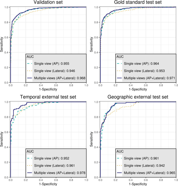
Area under the receiver operating characteristic curves of algorithm using multiple views (0.971, 0.978, and 0.965 for gold standard, temporal, and geographic external test sets, respectively) showed higher values than those using single view (0.964/0.953, 0.952/0.961, and 0.961/0.942 for AP view/lateral view of gold standard, temporal external, and geographic external test sets, respectively) in all test sets. The algorithm showed statistically significant higher specificity compared with radiologists (p = 0.018 and 0.012). There was substantial agreement between the algorithm and two radiologists and between two radiologists (κ = 0.79, 0.8, and 0.76).

Conclusion

The deep learning algorithm trained by multiple views showed better performance than that trained by single view. The diagnostic performance of the algorithm for detecting mastoiditis on mastoid series was similar to or higher than that of radiologists.

Introduction

Otomastoiditis is the second most common complication of acute otitis media (AOM) after tympanic membrane perforation [1]. Over the last several decades, the incidence of otomastoiditis as a complication of AOM has greatly decreased [1,2]. Nevertheless, improper management with antibiotics cannot prevent otomastoiditis and the incidence of otomastoiditis remains at approximately 1% [1]. Furthermore, the increasing numbers of immunocompromised patients who underwent organ transplantation surgery or received chemotherapy also increases the incidence of the occurrence of otomastoiditis. Diagnosis and early adequate treatment of otomastoiditis is very important, as the complications of otomastoiditis include sinus thrombosis and thrombophlebitis (transverse or sigmoid sinuses), encephalitis, and meningitis due to its proximity to intracranial structures [1,3].

High resolution temporal bone CT (TB CT) is the imaging modality of choice for the diagnosis of mastoiditis [4,5]. However, plain radiography of the mastoid (mastoid series) is still effective for screening mastoiditis in populations with very low prevalence such as pre-transplantation operation work up. Moreover, because the most commonly affected age group is the pediatric group, especially patients under two years old who are very sensitive to radiation exposure, simple radiography still has its role [2,6].

Because of the advancement in medical imaging techniques over the last century, there has been a tremendous increase in the amount of medical images. Simple radiographies are still the most commonly performed medical imaging until now due to both cost-effectiveness and clinical usefulness [7,8]. Therefore, simple radiographies take a large portion of radiologists’ work-loads [7–9]. In addition, accurate interpretation of simple radiographs requires an extensive amount of medical and radiologic knowledge and experience, as simple radiographies are composed of complex three-dimensional anatomic information projected into two-dimensional images [8].

Many studies have explored the application of deep learning technology to interpret simple radiographs (i.e., chest posterior-anterior [PA], Waters view, and mammography mediolateral oblique [MLO] view) to solve current problems in clinical practices including explosively increased radiologists’ work-loads and the intrinsic challenges of interpreting simple radiographs [10–14]. However, most studies used single-view images rather than multiple view images, unlike daily practices which usually use multiple view images in diagnosing diseases.

In this study, we developed a deep learning algorithm with a large dataset and evaluated its diagnostic performance in detecting mastoiditis with a mastoid series compared to the performance by head and neck radiologists. We also compared the diagnostic performance of the algorithm using multiple views (mastoid anterior-posterior [AP] view with lateral view) with that using single view (AP view or lateral view only).

Materials and methods

The Institutional Review Boards of Korea University Guro Hospital approved this study and informed consent was waived considering the retrospective design and anonymized data used in this study.

Dataset

Mastoid series for screening mastoiditis from 5,156 patients were collected from Korea University Guro Hospital (KUGH) that were taken between April 2003 and November 2018. Mastoid series were performed for screening mastoiditis not only in patients with suspected mastoiditis but also in patients planning to receive operations such as organ transplantation and cochlear implantation. In those cases, preoperative treatment of mastoiditis very important. The mastoid series consisted of an AP view and two lateral views (i.e., left and right lateral views). We excluded images that did not contain either the AP view or the bilateral views or the images that were uninterpretable due to artifacts. One hundred sixty-two patients were excluded according to these exclusion criteria. Among the remaining 4,994 patients, series of 396 patients who underwent TB CT examinations within seven days of the study date of their mastoid series were set aside as the gold standard test set. Majority of cases in the gold standard test set performed TB CT and mastoid series simultaneously. The mastoid series of the other 4,598 patients were used as the dataset for developing our deep learning algorithm. The training set and the validation set were generated by randomly dividing the dataset by 9:1.

We also collected temporally and geographically external test sets to further comprehensively verify the performance of the deep learning algorithm. The temporally external test set was collected from KUGH from December 2018 to April 2019 in 150 patients, and three patients were not included according to the exclusion criteria. The geographically external test sets were collected from Korea University Anam Hospital in 154 patients with the same time period.

We designed the deep learning algorithm to adopt an image set for one individual ear and to yield a classification result for the ear. An AP view was divided by the vertical bisector, and each half was fed into the algorithm as one individual training sample. A lateral view was directly used as an input training sample because the right and left lateral views already existed in separate images.

Labeling

Digital Imaging and Communication in Medicine (DICOM) files of the mastoid series were downloaded from the picture archiving and communication system (PACS) and all image data were anonymized for further analyses.

Two head and neck neuroradiologists (I.R. and H.N.J., both with 12 years of experience in this field) independently labeled mastoid series of the training and validation sets, temporal external test set, and geographic external test set and the labels were determined by consensus after the two radiologists discussed. The training and validation sets (mastoid series of 4,598 patients, total image sets of 9,196 ears) and the temporal (147 patients, 294 ears) and geographic (154 patients, 308 ears) external test sets were labeled based on the radiographic findings, whereas the gold standard test sets (mastoid series of 396 patients, image sets of 792 ears) were labeled based on the results of concurrent TB CT by one reader (I.R.).

For comparison of the diagnostic accuracy of the algorithm with head and neck neuroradiologists’ accuracy, two head and neck neuroradiologists with 12 years and 11 years of experience in this field (I.R. and L.S.) labeled mastoid series of the gold standard test set (images of 792 ears from 396 patients). The labeling criteria were same as the criteria used in labeling the training and validation sets.

Labeling TB CT and labeling mastoid series of gold standard test set were performed separately. Furthermore, mastoid series of gold standard test set were randomly mixed with other mastoid series in the training set and validation set when labeled.

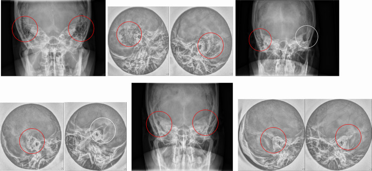
All the images in the dataset were labeled according to the following criteria in 5 categories: category 0, normal, clear mastoid air cells on both views (Fig 1A and 1B); category 1, mild, some haziness of mastoid air cells on any of AP view and lateral view (right ear in Fig 1C and 1D); category 2, severe, total haziness and sclerosis of mastoid air cells in both the AP and lateral views (Fig 1E and 1F); category 3, mastoidectomy state (left ear in Fig 1C and 1D); and category 4, unable to be labeled due to artifacts. Data sets labeled as category 3 or 4 were excluded from the training and validation sets and external validation sets. There were too few cases of postoperative images (category 3) to include for further analyses. However, postoperative cases (category 3) were included in the gold standard test set to evaluate how the algorithm classified the data. The gold standard test sets were labeled as category 0, normal; category 1, mild, soft tissue densities in some mastoid air cells; category 2, severe, soft tissue densities in near total air cells with sclerosis; and category 3, postoperative state according to the results of TB CT.

Fig 1. Typical images of each labeling category.

(a,b) AP view (a) and lateral view (b) show bilateral, clear mastoid air cells (red circles) with honey combing pattern of category 0. (c,d) right ear (red circles) of AP view (c) and lateral view (d) shows slightly increased haziness in mastoid air cells suggesting category 1 and left ear (white circles) of both views shows bony defects with air cavities suggesting category 3. (e, f) AP view (e) and lateral view (f) show bilateral, total haziness and sclerosis of mastoid air cells (red circles) suggesting category 2.

To simplify the interpretation of the results and to address the class imbalance issue due to the lack of positive samples, the labels were dichotomized with 0 as normal (category 0) and 1 as abnormal (category 1 and 2). The postoperative state (category 3) in the gold standard test set was also set as abnormal [1].

Deep learning algorithm

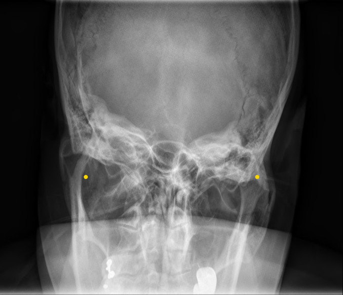
The AP view and the lateral views underwent the following preprocessing step before applying the deep learning algorithm. We cropped both ears in AP views assuming that all the images were taken at regular positions. For instance, the right ear in an AP view was cropped to have a size of 180×120 mm centered on 0.6 and 0.25 times the coordinates of the original image height and width and then the image was resized to 384×256 pixels. The left ear on the AP view was cropped in a similar way centered on the symmetrical coordinates. The right and left center points in the AP view are the points annotated in Fig 2. Outliers were excluded from the analyses. The lateral view was cropped to have a size of 140×140 mm at the center coordinates of the original image and was resized to 256×256 pixels. For data augmentation, horizontal and vertical shift and horizontal flipping were applied in the training set. We used the Pydicom library (Python Software Foundation; version 1.2.0) to process the images in the DICOM format.

Fig 2. Location of center points for right and left cropping in AP view.

The yellow dots represent the center points of cropping the right/left ears.

We performed the training on CUDA/cuDNN (versions 9.0 and 7.1, respectively) and TensorFlow library (version 1.12) for graphic processing unit acceleration on a Linux operating system. OS, CPU and GPU were Ubuntu 16.04, Intel® Xeon® CPU E5-2698 v4 @ 2.20GHz 80 cores, and Tesla V100-SXM2-32GB, respectively.

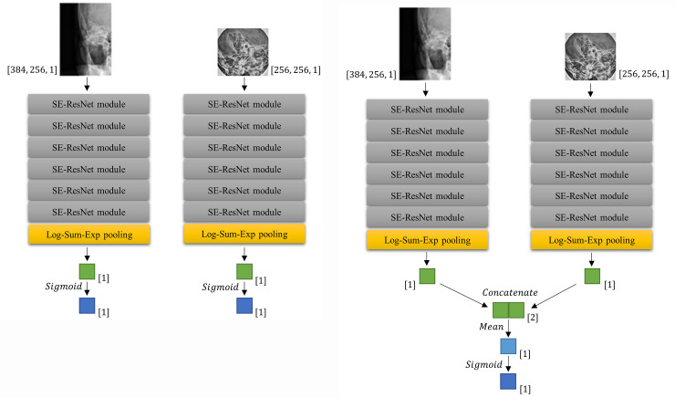
We designed two neural networks: i.e., one for a single view (an AP view or a lateral view, one image at a time, Fig 3A) and the other for multiple views (an AP view and two lateral views simultaneously, Fig 3B).

Fig 3. Network architectures for predicting mastoiditis.

The CNNs (convolutional neural networks) for single view (a) show a process in which AP and lateral views are separately trained in CNN. The CNN for multiple views (b) shows a process in which AP and lateral views are simultaneously trained. After Log-Sum-Exp pooling, the layers were also marked with dimensions. [1] means 1×1 size vector, and [2] means 1×2 size vector.

The convolutional neural network (CNN) for the single view consisted of a stack of six squeeze-and-excitation ResNet (SE-ResNet) modules [15] followed by the Log-Sum-Exp pooling [16] applied to the last SE-ResNet module (Fig 3A). Mastoiditis was predicted by applying Sigmoid function to the output of Log-Sum-Exp pooling. The weights of the network were initialized by Xavier initialization [17]. The learning rate decayed every 5,000 steps at the rate of 0.94 with the initial value of 0.01. The Cross-Entropy loss was minimized by employing the RMSProp optimizer [18], L2 regularization was applied to prevent overfitting, and batch size was set to 12.

The CNN for multiple views was constructed by combining the CNN applied to each view (Fig 3B). Each CNNs for single view were combined by concatenate and average the output of Log-Sum-Exp pooling of each single view network without additional weight. Finally, Sigmoid function was applied at the averaged value to predict mastoiditis. To enhance efficacy, we started training with the weights obtained from the training of each single views for the pre-training [19]. The learning rate decayed every 1,000 steps at the rate of 0.04 with 0.005 as the initial value smaller than in CNN for single view to fine-tune already gained weights. Loss function, optimizer, regularization term, and batch size were the same as for the CNN for single view. The CNNs we implemented were uploaded to the public repository (https://github.com/djchoi1742/Mastoid_CNN).

A class activation map was generated to identify which parts of the original image were activated when the CNN recognized mastoiditis. In the CNN both single view and multiple views, the class activation mappings of each view were obtained by resizing to their input size using bilinear interpolation based on the results immediately before the Log-Sum-Exp pooling step in Fig 3A and 3B. The class activation mappings were obtained by applying rectified linear activation function (ReLU) to these results in order to confirm the region strongly predicted to have mastoiditis. Since the presence or absence of mastoiditis was calculated by Sigmoid function as a final output, the region predicted to have mastoiditis was detected only on the class activation mapping for the image judged to have mastoiditis. Otherwise, no region was detected.

Statistical analysis

We used DeLong’s test for two correlated receiver operating characteristic curves (ROC curves) [20] to compare the diagnostic performance of the algorithm using multiple views with that using a single view. Sensitivity, specificity, and area under the receiver operating characteristic curve (AUC) were used as measures to evaluate the performance of the deep learning algorithm. We applied three cut-off points calculated from the validation set to the test datasets; i.e., the optimal cut-off point obtained by Youden’s J statistic, the cut-off point at which sensitivity was 95%, and the cut-off point at which specificity was 95%. Clopper-Pearson method [21] was applied to calculate 95% confidence intervals for sensitivity and specificity, and the method of DeLong et al. [20] was used to calculate 95% confidence intervals of AUC.

McNemar’s test for sensitivity and specificity was used to compare the diagnostic performance between the deep learning algorithm and the radiologist results. Cohen’s κ coefficient was used to evaluate the agreement between the results diagnosed by deep learning algorithm and the radiologist diagnosis. The level of agreement was interpreted as poor if κ was less than 0; slight, 0 to 0.20; fair, 0.21 to 0.40; moderate, 0.41 to 0.60; substantial, 0.61 to 0.80; and almost perfect, 0.81 to 1.00 [22]. Qualitative analysis was performed by showing the CNN class activation map [23].

All statistical analyses were performed with R statistical software version 3.6.1 (The R Foundation for Statistical Computing, Vienna, Austria). A p-value less than 0.05 was considered statistically significant.

Results

The baseline characteristics of training set, validation set, gold standard test set, temporal external test set, and geographic external test set are shown in Table 1. There was no statistical difference in label distribution between the temporal external test set and geographic external test set (P = 0.118). The ROC curves and DeLong’s test for two correlated ROC curves comparing the diagnostic performance between the algorithm using single view and the algorithm using multiple views in each dataset are shown in Fig 4 and Table 2, respectively. In comparison of the diagnostic performance of deep learning algorithm using multiple views (AP view and lateral view) with that using a single view (AP view or lateral view only), AUCs from the multiple views showed statistically significant higher values than AUCs using a single view (AP view or lateral view only) in the validation set and all test sets (gold standard test set, temporally external test set, and geographically external test set), except for AUC using a single AP view in the geographic external test set. Even the AUC using AP view in the geographic external test set also showed a lower value than AUC using multiple views; however, statistical significance was not shown (P = 0.246).

Table 1. Baseline characteristics of all data sets.

Characteristic			Training set (n = 8278)	Validation set (n = 918)	Test sets
					Gold standard test set (n = 792)	Temporal external test set (n = 294)	Geographic external test set (n = 308)
Number of patients			4139	459	396	147	154
Age
	<20 years		322	35	40	4	4
	20~29 years		262	32	16	4	7
	30~39 years		444	68	47	10	15
	40~49 years		912	97	85	21	28
	50~59 years		1131	114	119	60	59
	60~69 years		774	80	55	37	26
	70~79 years		258	30	27	8	14
	≥80 years		36	3	7	3	1
Sex
	Female		2353	247	225	70	69
	Male		1786	212	171	77	85
Label (based on conventional radiography)
	0, Normal		3155	349	261	159	175
	1, Abnormal		5123	569	531	135	133
		Mild	1806	200	129	56	44
		Severe	3317	369	402	76	89
		Postop	-	-	-	3	-
Label (based on CT)
	0, Normal		-	-	353	-	-
	1, Abnormal		-	-	439	-	-
		Mild	-	-	157	-	-
		Severe	-	-	258	-	-
		Postop	-	-	24	-	-
κ coefficient between two reviewers			0.78	0.77	0.76	0.79	0.79

Fig 4. The receiver operating characteristic curves (ROC curves) for validation set and three test sets.

The area under the ROC curves (AUCs) using the multiple views show statistically significant higher values than AUCs using a single view (AP view or lateral view only) in the validation set and all test sets.

Table 2. Comparison of the diagnostic performance between the algorithm using single view and the algorithm using multiple views in each data set based on labels by conventional radiography.

Dataset	Comparison	AUC (single view)	AUC (multiple views)	P*
Validation set	Single view (AP) vs Multiple views	0.955 (0.943–0.968)	0.968 (0.959–0.977)	<0.001*
	Single view (Lateral) vs Multiple views	0.946 (0.932–0.959)		<0.001*
Gold standard test set	Single view (AP) vs Multiple views	0.964 (0.953–0.975)	0.971 (0.962–0.981)	0.017*
	Single view (Lateral) vs Multiple views	0.953 (0.940–0.966)		<0.001*
Temporal external test set	Single view (AP) vs Multiple views	0.952 (0.931–0.974)	0.978 (0.965–0.990)	0.002*
	Single view (Lateral) vs Multiple views	0.961 (0.942–0.980)		0.004*
Geographic external test set	Single view (AP) vs Multiple views	0.961 (0.942–0.980)	0.965 (0.948–0.981)	0.246
	Single view (Lateral) vs Multiple views	0.942 (0.918–0.966)		0.003*

Data is shown to three decimal places, with the 95% confidence interval in parentheses.

AUC: Area under the receiver operating characteristic (ROC) curves.

P*: P-value of one-side DeLong’s test for two correlated ROC curves (Alternative hypothesis: AUC of multiple views was greater than AUC of single view).

*:<0.05 was significant.

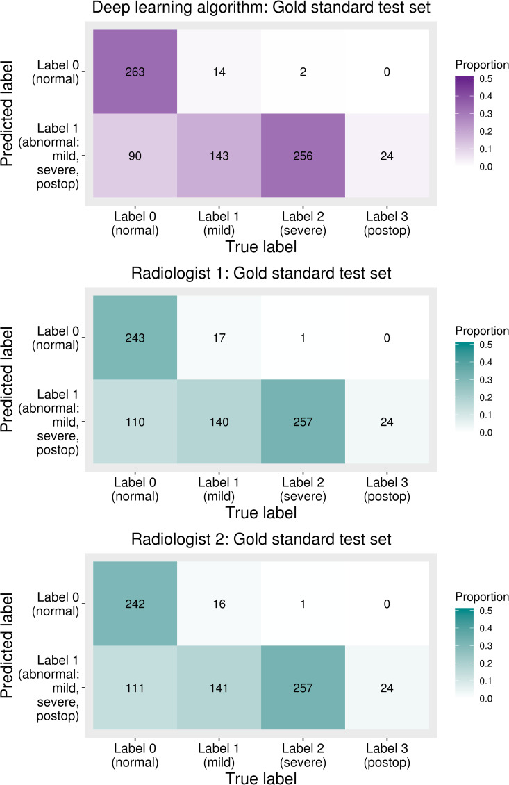
The sensitivity and specificity calculated based on the optimal cut-off point determined by Youden’s J statistic, the cut-off point for an expected sensitivity of 95%, and the cut-off point for an expected specificity of 95% described above to evaluate the diagnostic accuracy of the deep learning algorithm and radiologist results are summarized in Table 3. Usually, cut-off point is derived from the validation set assuming that we do not know the exact distribution of the test set [24]. This data was based on labels diagnosed with TB CT. With the optimal cut-off point, the sensitivity and specificity of the gold standard test set diagnosed by the deep learning algorithm were 96.4% (423/439, 95% confidence interval, 94.1% - 97.9%) and 74.5% (263/353, 95% confidence interval, 69.6% - 79.0%), respectively. The sensitivity of the deep learning algorithm was not significantly different from those of the radiologists (p-value = 0.752 and 1.000). However, the specificity diagnosed by the deep learning algorithm was significantly higher than those of the radiologists (p-value = 0.018 and 0.012, respectively). In addition, confusion matrices between the prediction of the deep learning algorithm and radiologists’ predictions based on the reference standard are shown in Fig 5. Gold standard labels were divided into categories 1, 2, and 3 to check how the deep learning algorithm and radiologists predicted normal or abnormal and to see the detailed results of each label. The postoperative category (category 3) was not included in training; however, this was considered abnormal in the gold standard test set. Severe (category 2) labels were predicted as abnormal except for two cases, and mild (category 1) labels were predicted as abnormal at about 90%; all postoperative data were predicted as abnormal.

Table 3. Comparison of diagnostic performance for gold standard test set between the deep learning algorithm (using multiple views) and radiologists based on the labels by standard reference (temporal bone CT).

Reader		Sensitivity	Pse	Specificity	Psp
Deep learning algorithm	Optimal cutoff	96.4% (423/439, 94.1–97.9%)		74.5% (263/353, 69.6–79.0%)
	Cutoff for 95% sensitivity	98.6% (433/439, 97.0–99.5%)		58.9% (208/353, 53.6–64.1%)
	Cutoff for 95% specificity	95.7% (420/439, 93.3–97.4%)		79.3% (280/353, 74.7–83.4%)
Radiologist	Radiologist 1	95.9% (421/439, 93.6–97.6%)	0.752	68.8% (243/353, 63.7–73.6%)	0.018*
	Radiologist 2	96.1% (422/439, 93.9–97.7%)	1.000	68.6% (242/353, 63.4–73.4%)	0.012*

Data are percentages and nominator/denominator, and 95% confidence interval in the parentheses.

P^se,P^sp: P values for comparing sensitivities/specificities between the deep learning algorithm based on optimal cutoff and the radiologists were determined by using McNemar’s test.

*:<0.05 was significant.

Fig 5. Confusion matrices between predicted labels and temporal bone CT based gold-standard labels.

Predicted labels are normal (label 0) or abnormal (label 1) since the deep learning algorithm was trained based on the dichotomized data (e.g., normal or abnormal).

There was substantial agreement between the radiologists and deep learning algorithm (κ coefficient between radiologist 1 and deep learning algorithm: 0.79, κ coefficient between radiologist 2 and deep learning algorithm, 0.8) in the gold standard test set. In addition, the κ coefficient between radiologist 1 and radiologist 2 was 0.76 in the same test set.

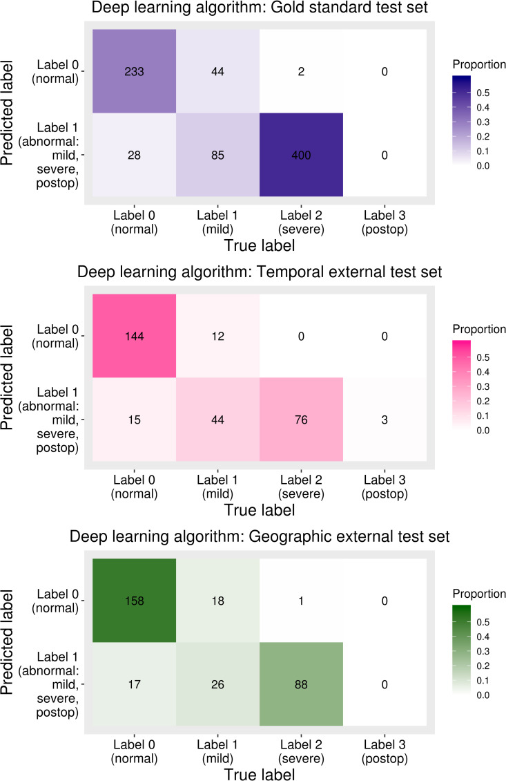
The AUC, sensitivity, and specificity of the test sets were calculated based on the labels diagnosed based on both AP view and lateral view. The AUC of the deep learning algorithm for gold standard test set, temporal external test set, and geographic external test set was 0.97 (95% confidence interval, 0.96–0.98), 0.98 (95% confidence interval, 0.97–0.99), and 0.97 (95% confidence interval, 0.95–0.98), respectively. The sensitivity and specificity of the deep learning algorithm of the three test sets are shown in Table 4. The sensitivity and specificity of the gold standard test set were 91.3% (95% confidence interval, 88.6–93.6%) and 89.3% (95% confidence interval, 84.9–92.8%), respectively. The sensitivity and specificity of the temporal external test set were 91.1% (95% confidence interval, 85.0–95.3%) and 90.6% (95% confidence interval, 84.9–94.6%), respectively, and those of the geographic external test set were 85.7% (95% confidence interval, 78.6–91.2%) and 90.3% (95% confidence interval, 84.9–94.2%), respectively. Under the optimal cut-off of the validation set, the sensitivity of the geographic test set was somewhat lower than that of the other two test sets. Confusion matrices between the conventional radiography-based label and predictions of the deep learning algorithm are shown in Fig 6. In all three test sets, the proportion of cases incorrectly diagnosed as normal in the mild labeled group was larger than that in the severe labeled group.

Table 4. Diagnostic performance of deep learning algorithm in all test sets based on labels by conventional radiography.

Diagnostic performance		Gold standard test set	Temporal external test set	Geographic external test set
AUC		0.971 (0.962–0.981)	0.978 (0.965–0.990)	0.965 (0.948–0.981)
Optimal cutoff	Sensitivity	91.3% (485/531, 88.6–93.6%)	91.1% (123/135, 85.0–95.3%)	85.7% (114/133, 78.6–91.2%)
	Specificity	89.3% (233/261, 84.9–92.8%)	90.6% (144/159, 84.9–94.6%)	90.3% (158/175, 84.9–94.2%)
Cutoff for 95% sensitivity	Sensitivity	96.8% (514/531, 94.9–98.1%)	97.8% (132/135, 93.6–99.5%)	97.0% (129/133, 92.5–99.2%)
	Specificity	75.5% (197/261, 69.8–80.6%)	79.2% (126/159, 72.1–85.3%)	80.6% (141/175, 73.9–86.2%)
Cutoff for 95% specificity	Sensitivity	89.3% (474/531, 86.3–91.8%)	90.4% (122/135, 84.1–94.8%)	85.0% (113/133, 77.7–90.6%)
	Specificity	92.7% (242/261, 88.9–95.6%)	93.7% (149/159, 88.7–96.9%)	91.4% (160/175, 86.3–95.1%)

Data are percentages and nominator/denominator and/or 95% confidence interval in the parentheses.

AUC: Area under the receiver operating characteristic curve.

Fig 6. Confusion matrices between the predicted labels of a deep learning algorithm and labels based on conventional radiography.

In all test sets, the proportion of the incorrectly diagnosed cases was larger in mild labeled group (category 1) than in severe labeled group (category 2).

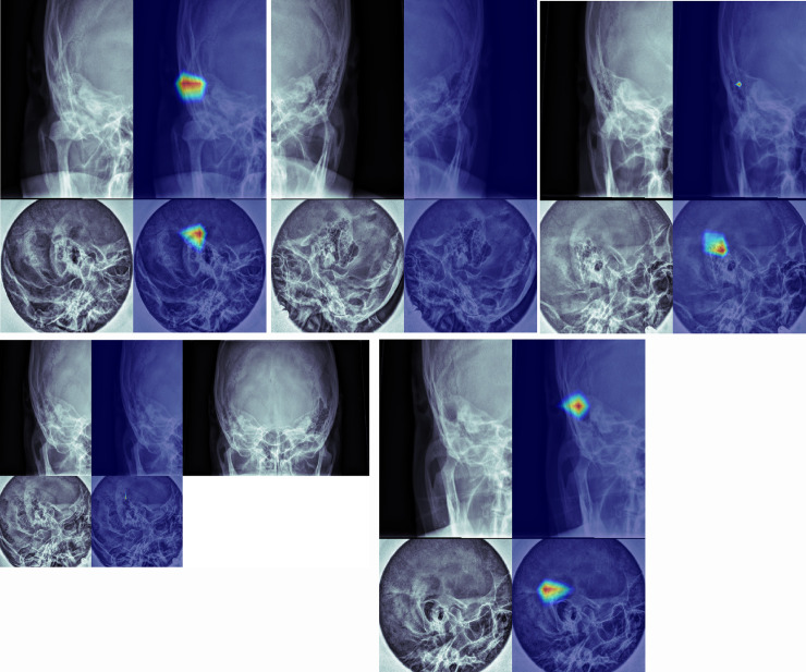
Class activation mappings of the sample images are shown in Fig 7 (true positive (a), true negative (b), false positive (c), false negative (d), and postoperative state (e) examples). These class activation mappings are obtained from the CNN for multiple view. If deep learning algorithm determined a case to be normal, neither AP view nor lateral view detected a specific region of the image (Fig 7B and 7D). In contrast, a case was determined as mastoiditis, lesion-related regions were detected in at least one of AP and lateral views (Fig 7A, 7C and 7E).

Fig 7. Class activation mappings of true positive (a), true negative (b), false positive (c), false negative (d), and postoperative state (e) examples.

(a) Lesion related regions in mastoid air cells are detected on both AP view and lateral view. (b) No specific region is detected in either AP view or lateral view. (c) A false lesion related region is detected on lateral view. (d) Equivocal haziness is suspected on both views. The algorithm diagnosed this case as normal. An AP view with bilateral sides (right upper) shows marked asymmetry suggesting abnormality in right side. (e) Both views show lesion related regions.

Although not considered in training, how the deep leaning algorithm determines both views that were labeled as postoperative state based on reference standard was also analyzed and the algorithm determined all the postoperative cases as abnormal (Fig 7E). In both views, abnormal regions in images were at the mastoid air cells.

Discussion

Over the last couple of years, great advancement and progression of deep learning technologies have become integrated into not only medical fields but also all other industrial fields [25–28]. Radiology is one of the most promising fields with respect to applications for new deep learning technologies, and many previous studies have suggested vast possibilities for new directions in this field [29–33].

The amount of medical images continues to increase explosively, and the average radiologist reads more than 100 simple radiograph examinations per day in the United States [7,8]. Application of deep learning technologies to radiology can be clinically very beneficial to radiologists and can be a new academic field in radiology.

In the present study, the deep learning algorithm trained by multiple views (mastoid AP view with lateral view) of the lesion showed better performance than that trained by single view (mastoid AP view or lateral view). This is very meaningful in the interpretation of medical images, since radiologists usually use multiple images rather than a single image in clinical practice for diagnosing diseases. For example, radiologists frequently use chest PA with a lateral view for evaluation of lung diseases, Waters view with Caldwell view and lateral view for evaluation of paranasal sinusitis, and MLO view with craniocaudal (CC) view for breast cancer screening using mammography. This is not limited to simple radiographs. For advanced imaging modalities, multiphase images of a lesion are used in CT scans and even multiphase with multiple sequences of a lesion are used in MR imaging.

In this study, the deep learning algorithm could diagnose mastoiditis with accuracy similar to or higher than that of head and neck radiologists. The sensitivity (96.4%) and specificity (74.5%) of the deep learning algorithm were higher than those of head and neck neuroradiologists (sensitivities, 95.9% and 96.1%; specificities, 68.8% and 68.6%) in diagnosing mastoiditis using TB CT as the standard reference. In terms of specificity, there was a statistically significant difference.

Even though the deep learning algorithm cannot directly replace radiologists in diagnosing diseases with images, radiologists’ work-loads can be reduced by the development of deep learning algorithms with very high sensitivity. In this case, algorithms would interpret a large portion of images and radiologists would check only positive or equivocal cases. This workflow would be especially helpful for areas with few radiologists or locations where access to radiologists is cost prohibitive [8,12]. Since the simple radiographs still take major part of radiologists’ work-loads these days, deep learnings using simple radiographs are especially meaningful.

In this study, we did not simply want to evaluate the ability of the deep learning algorithm to diagnose mastoiditis with mastoid series. Unlike anatomic locations that have been studied during the last several years, including breast, paranasal sinuses, and even lung, mastoid air cells show considerable variations in terms of pneumatization between individuals and they change greatly during age [34–37]. The mastoid lateral view is also a summation of multiple complex anatomic structures such as mastoid air cells, temporo-mandibular joints, complex skull base, and even auricles. Even though there were a great deal of variations in mastoid air cells and complex anatomic structures around mastoid air cells, in this study, the class activation maps consistently showed the exact location of diseased mastoid air cells. This showed the possibility of deep learning algorithms for use in the interpretation of medical images that usually have huge anatomic diversities and variations, as long as the algorithms are trained with large enough datasets.

This study has several limitations. First, the training set and validation set had no reference standards (TB CT), and only the gold standard test set had TB CT data as a reference standard. However, the diagnostic performance of the deep learning algorithm using the gold standard test set showed better results than that using the validation set. The diagnostic performance using the external test sets also showed similar results. Second, if the deep learning algorithm found regions related to mastoiditis in only one of the two views, the algorithm often misdiagnosed a normal case as having mastoiditis and vice versa. This was similar to the actual image interpretation processes in which both views were read at the same time by head and neck radiologists. Third, radiologists used mastoid AP views with both sides of mastoid air cells simultaneously in interpreting images as used in clinical practices. In contrast, the deep learning algorithm used cropped images of the unilateral mastoid. However, this means that the deep learning algorithm was at a marked disadvantage compared with radiologists. Because there is no significant anatomic variation between bilateral mastoid air cells in one person, while there are huge variations between individuals [35], assessing symmetry of bilateral mastoid air cells in one person is very useful in the diagnosis of mastoiditis. Despite this issue, the diagnostic performance of the deep learning algorithm was similar to or higher than that of radiologists. In addition, the assessment of symmetry in human bodies on radiologic studies is a frequently used method in imaging diagnosis of diseases. Therefore, we are now developing deep learning algorithms to evaluate the symmetry of anatomies in radiologic images.

Conclusion

This study showed that deep learning algorithm trained by multiple views of the lesion showed better performance than that trained by single view. Despite considerable anatomic variations of mastoid air cells between individuals and summation of complex anatomic structures in mastoid series, deep learning algorithm depicted the exact location of diseased mastoid air cells and showed a similar or higher performance, as compared with head and neck radiologists. Based on this result, deep learning algorithms might be applied to the interpretation of medical images that usually have huge anatomic diversities and variations, as long as trained by large enough datasets.

Supporting information

S1 File

(ZIP)

S2 File

(ZIP)

S3 File

(ZIP)

Data Availability

All relevant data are within the manuscript and its Supporting Information files.

Funding Statement

IR, Grant No: 2017R1C1B5076240, National Research Foundation of Korea, URL: www.nrf.re.kr; KJL, Grant No: 13-2019-006, Seoul National University Bundang Hospital Research Fund, URL: www.snubh.org. The funders had no role in study design, data collection and analysis, decision to publish, or preparation of the manuscript.

References

• 1.Palma S, Bovo R, Benatti A, Aimoni C, Rosignoli M, Libanore M, et al. Mastoiditis in adults: a 19-year retrospective study. Eur Arch Otorhinolaryngol. 2014;271:925–931. 10.1007/s00405-013-2454-8 [DOI] [PubMed] [Google Scholar]
• 2.Popescu C, Ionita E, Mogoanta CA, Simionescu C, Patru E. Clinical and histopathological aspects in otomastoiditis. Rom J Morphol Embryol. 2009;50:453–460. [PubMed] [Google Scholar]
• 3.van den Aardweg MT, Rovers MM, de Ru JA, Albers FW, Schilder AG. A systematic review of diagnostic criteria for acute mastoiditis in children. Otol Neurotol. 2008;29:751–757. 10.1097/MAO.0b013e31817f736b [DOI] [PubMed] [Google Scholar]
• 4.Mafee MF, Singleton EL, Valvassori GE, Espinosa GA, Kumar A, Aimi K. Acute otomastoiditis and its complications: role of CT. Radiology. 1985;155:391–397. 10.1148/radiology.155.2.3983389 [DOI] [PubMed] [Google Scholar]
• 5.Rho MH, Kim DW, Kim SS, Sung YS, Kwon JS, Lee SW. Tuberculous otomastoiditis on high-resolution temporal bone CT: comparison with nontuberculous otomastoiditis with and without cholesteatoma. AJNR Am J Neuroradiol. 2007;28:493–496. [PMC free article] [PubMed] [Google Scholar]
• 6.Oestreicher-Kedem Y, Raveh E, Kornreich L, Popovtzer A, Buller N, Nageris B. Complications of mastoiditis in children at the onset of a new millennium. Ann Otol Rhinol Laryngol. 2005;114:147–152. 10.1177/000348940511400212 [DOI] [PubMed] [Google Scholar]
• 7.Kamel SI, Levin DC, Parker L, Rao VM. Utilization Trends in Noncardiac Thoracic Imaging, 2002–2014. J Am Coll Radiol. 2017;14:337–342. 10.1016/j.jacr.2016.09.039 [DOI] [PubMed] [Google Scholar]
• 8.Lee SM, Seo JB, Yun J, Cho YH, Vogel-Claussen J, Schiebler ML, et al. Deep Learning Applications in Chest Radiography and Computed Tomography: Current State of the Art. J Thorac Imaging. 2019;34:75–85. 10.1097/RTI.0000000000000387 [DOI] [PubMed] [Google Scholar]
• 9.Hong AS, Levin D, Parker L, Rao VM, Ross-Degnan D, Wharam JF. Trends in Diagnostic Imaging Utilization among Medicare and Commercially Insured Adults from 2003 through 2016. Radiology. 2020;294:342–350. 10.1148/radiol.2019191116 [DOI] [PMC free article] [PubMed] [Google Scholar]
• 10.Kim HG, Lee KM, Kim EJ, Lee JS. Improvement diagnostic accuracy of sinusitis recognition in paranasal sinus X-ray using multiple deep learning models. Quant Imaging Med Surg. 2019;9:942–951. 10.21037/qims.2019.05.15 [DOI] [PMC free article] [PubMed] [Google Scholar]
• 11.Kim Y, Lee KJ, Sunwoo L, Choi D, Nam CM, Cho J, et al. Deep Learning in Diagnosis of Maxillary Sinusitis Using Conventional Radiography. Invest Radiol. 2019;54:7–15. 10.1097/RLI.0000000000000503 [DOI] [PubMed] [Google Scholar]
• 12.Lakhani P, Sundaram B. Deep Learning at Chest Radiography: Automated Classification of Pulmonary Tuberculosis by Using Convolutional Neural Networks. Radiology. 2017;284:574–582. 10.1148/radiol.2017162326 [DOI] [PubMed] [Google Scholar]
• 13.Singh R, Kalra MK, Nitiwarangkul C, Patti JA, Homayounieh F, Padole A, et al. Deep learning in chest radiography: Detection of findings and presence of change. PLoS One. 2018;13(10):e0204155 10.1371/journal.pone.0204155 [DOI] [PMC free article] [PubMed] [Google Scholar]
• 14.Yala A, Schuster T, Miles R, Barzilay R, Lehman C. A Deep Learning Model to Triage Screening Mammograms: A Simulation Study. Radiology. 2019:293;38–46. 10.1148/radiol.2019182908 [DOI] [PubMed] [Google Scholar]
• 15.Hu J, Shen L, Albanie S, Sun G, Wu E, editors. Squeeze-andexcitation networks. IEEE conference on computer vision and pattern recognition; 2018. [Google Scholar]
• 16.Yao L, Prosky J, Poblenz E, Covington B, Lyman K. Weakly supervised medical diagnosis and localization from multiple resolutions. arXiv preprint arXiv. 2018:180307703. [Google Scholar]
• 17.Glorot X, Bengio Y, editors. Understanding the difficulty of training deep feedforward neural networks. the thirteenth international conference on artificial intelligence and statistics; 2010. [Google Scholar]
• 18.Hinton G, Srivastava N, Swersky K. Neural networks for machine learning lecture 6a overview of mini-batch gradient descent 2012. Available from:https://www.cs.toronto.edu/~hinton/coursera/lecture6/lec6.pdf. [Google Scholar]
• 19.Yosinski J, Clune J, Bengio Y, and Lipson H. How transferable are features in deep neural networks? In Advances in neural information processing systems 27 2014, 3320–3328. [Google Scholar]
• 20.DeLong ER, DeLong DM, Clarke-Pearson DL. Comparing the areas under two or more correlated receiver operating characteristic curves: a nonparametric approach. Biometrics. 1988;44:837–845. [PubMed] [Google Scholar]
• 21.Clopper CJ, Pearson ES. The use of confidence or fiducial limits illustrated in the case of the binomial. Biometrika. 1934;26:404–413. [Google Scholar]
• 22.McHugh ML. Interrater reliability: the kappa statistic. Biochem Medica. 2012;22:276–282. [PMC free article] [PubMed] [Google Scholar]
• 23.Zhou B, Khosla A, Lapedriza A, editors. Learning deep features for discriminative localization. IEEE Conference on Computer Vision and Pattern Recognition; 2016. [Google Scholar]
• 24.Gulshan V, Peng L, Coram M, et al. Development and validation of a deep learning algorithm for detection of diabetic retinopathy in retinal fundus photographs. JAMA. 2016;316:2402–2410. 10.1001/jama.2016.17216 [DOI] [PubMed] [Google Scholar]
• 25.Hinton G, Deng L, Yu D, Dahl GE, Mohamed AR, Jaitly N, et al. Deep Neural Networks for Acoustic Modeling in Speech Recognition. Ieee Signal Proc Mag. 2012;29:82–97. [Google Scholar]
• 26.Leung MKK, Xiong HY, Lee LJ, Frey BJ. Deep learning of the tissue-regulated splicing code. Bioinformatics. 2014;30:121–129. 10.1093/bioinformatics/btt614 [DOI] [PMC free article] [PubMed] [Google Scholar]
• 27.Ren SQ, He KM, Girshick R, Sun J. Faster R-CNN: Towards Real-Time Object Detection with Region Proposal Networks. Ieee T Pattern Anal. 2017;39:1137–1149. 10.1109/TPAMI.2016.2577031 [DOI] [PubMed] [Google Scholar]
• 28.Zhao R, Yan RQ, Chen ZH, Mao KZ, Wang P, Gao RX. Deep learning and its applications to machine health monitoring. Mech Syst Signal Pr. 2019;115:213–237. [Google Scholar]
• 29.Aldoj N, Lukas S, Dewey M, Penzkofer T. Semi-automatic classification of prostate cancer on multi-parametric MR imaging using a multi-channel 3D convolutional neural network. Eur Radiol. 2020:30;1243–1253. 10.1007/s00330-019-06417-z [DOI] [PubMed] [Google Scholar]
• 30.Grovik E, Yi D, Iv M, Tong E, Rubin D, Zaharchuk G. Deep learning enables automatic detection and segmentation of brain metastases on multisequence MRI. J Magn Reson Imaging. 2020:51;175–182. 10.1002/jmri.26766 [DOI] [PMC free article] [PubMed] [Google Scholar]
• 31.Kiryu S, Yasaka K, Akai H, Nakata Y, Sugomori Y, Hara S, et al. Deep learning to differentiate parkinsonian disorders separately using single midsagittal MR imaging: a proof of concept study. Eur Radiol. 2019:29;6891–6899. 10.1007/s00330-019-06327-0 [DOI] [PubMed] [Google Scholar]
• 32.Ko SY, Lee JH, Yoon JH, Na H, Hong E, Han K, et al. Deep convolutional neural network for the diagnosis of thyroid nodules on ultrasound. Head Neck. 2019;41:885–891. 10.1002/hed.25415 [DOI] [PubMed] [Google Scholar]
• 33.Lee JH, Baek JH, Kim JH, Shim WH, Chung SR, Choi YJ, et al. Deep Learning-Based Computer-Aided Diagnosis System for Localization and Diagnosis of Metastatic Lymph Nodes on Ultrasound: A Pilot Study. Thyroid. 2018;28:1332–1338. 10.1089/thy.2018.0082 [DOI] [PubMed] [Google Scholar]
• 34.Koc A, Ekinci G, Bilgili AM, Akpinar IN, Yakut H, Han T. Evaluation of the mastoid air cell system by high resolution computed tomography: three-dimensional multiplanar volume rendering technique. J Laryngol Otol. 2003;117:595–598. 10.1258/002221503768199906 [DOI] [PubMed] [Google Scholar]
• 35.Lee DH, Jun BC, Kim DG, Jung MK, Yeo SW. Volume variation of mastoid pneumatization in different age groups: a study by three-dimensional reconstruction based on computed tomography images. Surg Radiol Anat. 2005;27:37–42. 10.1007/s00276-004-0274-7 [DOI] [PubMed] [Google Scholar]
• 36.Luntz M, Malatskey S, Tan M, Bar-Meir E, Ruimi D. Volume of mastoid pneumatization: three-dimensional reconstruction with ultrahigh-resolution computed tomography. Ann Otol Rhinol Laryngol. 2001;110(5 Pt 1):486–490. 10.1177/000348940111000516 [DOI] [PubMed] [Google Scholar]
• 37.Todd NW, Pitts RB, Braun IF, Heindel H. Mastoid size determined with lateral radiographs and computerized tomography. Acta Otolaryngol. 1987;103:226–231. [PubMed] [Google Scholar]
Decision Letter 0
Yuchen Qiu
18 Jun 2020
PONE-D-20-11571
Deep learning in diagnosis of mastoiditis using multiple mastoid views
PLOS ONE
Dear Dr. Ryoo,
Thank you for submitting your manuscript to PLOS ONE. After careful consideration, we feel that it has merit but does not fully meet PLOS ONE’s publication criteria as it currently stands. Therefore, we invite you to submit a revised version of the manuscript that addresses the points raised during the review process.
Please submit your revised manuscript by Aug 02 2020 11:59PM. If you will need more time than this to complete your revisions, please reply to this message or contact the journal office at plosone@plos.org. When you're ready to submit your revision, log on to https://www.editorialmanager.com/pone/ and select the 'Submissions Needing Revision' folder to locate your manuscript file.
Please include the following items when submitting your revised manuscript:
• A rebuttal letter that responds to each point raised by the academic editor and reviewer(s). You should upload this letter as a separate file labeled 'Response to Reviewers'.
• A marked-up copy of your manuscript that highlights changes made to the original version. You should upload this as a separate file labeled 'Revised Manuscript with Track Changes'.
• An unmarked version of your revised paper without tracked changes. You should upload this as a separate file labeled 'Manuscript'.
If you would like to make changes to your financial disclosure, please include your updated statement in your cover letter. Guidelines for resubmitting your figure files are available below the reviewer comments at the end of this letter.
If applicable, we recommend that you deposit your laboratory protocols in protocols.io to enhance the reproducibility of your results. Protocols.io assigns your protocol its own identifier (DOI) so that it can be cited independently in the future. For instructions see: http://journals.plos.org/plosone/s/submission-guidelines#loc-laboratory-protocols
We look forward to receiving your revised manuscript.
Kind regards,
Yuchen Qiu, Ph.D.
Academic Editor
Journal Requirements:
When submitting your revision, we need you to address these additional requirements.
1. Please ensure that your manuscript meets PLOS ONE's style requirements, including those for file naming. The PLOS ONE style templates can be found at
https://journals.plos.org/plosone/s/file?id=wjVg/PLOSOne_formatting_sample_main_body.pdf and
https://journals.plos.org/plosone/s/file?id=ba62/PLOSOne_formatting_sample_title_authors_affiliations.pdf
2. Please include captions for your Supporting Information files at the end of your manuscript, and update any in-text citations to match accordingly. Please see our Supporting Information guidelines for more information: http://journals.plos.org/plosone/s/supporting-information.
[Note: HTML markup is below. Please do not edit.]
Reviewers' comments:
Reviewer's Responses to Questions
Comments to the Author
1. Is the manuscript technically sound, and do the data support the conclusions?
The manuscript must describe a technically sound piece of scientific research with data that supports the conclusions. Experiments must have been conducted rigorously, with appropriate controls, replication, and sample sizes. The conclusions must be drawn appropriately based on the data presented.
Reviewer #1: Yes
Reviewer #2: Yes
Reviewer #3: Partly
**********
2. Has the statistical analysis been performed appropriately and rigorously?
Reviewer #3: Yes
3. Have the authors made all data underlying the findings in their manuscript fully available?
The PLOS Data policy requires authors to make all data underlying the findings described in their manuscript fully available without restriction, with rare exception (please refer to the Data Availability Statement in the manuscript PDF file). The data should be provided as part of the manuscript or its supporting information, or deposited to a public repository. For example, in addition to summary statistics, the data points behind means, medians and variance measures should be available. If there are restrictions on publicly sharing data—e.g. participant privacy or use of data from a third party—those must be specified.
4. Is the manuscript presented in an intelligible fashion and written in standard English?
PLOS ONE does not copyedit accepted manuscripts, so the language in submitted articles must be clear, correct, and unambiguous. Any typographical or grammatical errors should be corrected at revision, so please note any specific errors here.
Reviewer #2: No
5. Review Comments to the Author
Please use the space provided to explain your answers to the questions above. You may also include additional comments for the author, including concerns about dual publication, research ethics, or publication ethics. (Please upload your review as an attachment if it exceeds 20,000 characters)
Reviewer #1: This article compared the diagnostic performance of mastoiditis with Squeeze-and-Excitation Networks(SENet) trained by single view radiographic images with that trained by multiple view images and with radiologists' rating. The reference standards are the two radiologists' rating on plain radiography. Because the specificity of diagnosing mastoiditis is low on the plain radiography, the authors also provide the testing results based on radiologists' rating from CT images. The algorithms trained on 4139 patients and tested on three testing sets and showed the SENet trained on by multiple views images achieved better performance than that trained by single view images. Compare with reference standard from CT, the SENet showed similar sensitivity with radiologists and higher specificity than radiologists.
However, the authors need to find similar literature as benchmarks to compare the performance.
Authors write all data are fully available without restriction. How about the image data and labels?
The title is too general.
Line 3 add anteroposterior (AP)
Line 9 add case numbers for training and validation sets.
Line 15 add AUC values
Rephase the sentence on line 22.
Line 43 This also contributes to a tremendous increase in radiologists’ work
loads. What is this refer to?
Line 66 What is the inclusion criteria in detail? Do somehow mastoiditis need a screening? Why the mastoid series didn't include any other diseases?
What are the criteria for those patients underwent TB CT after radiography? Do you think those patients' plain radiographic images are different from the rest?
What if the two radiologists labeled different?
Show kappa coefficients between two radiologists for each dataset.
Why I.R. and L.S. instead of H.N.J. label the gold standard test set again or for CT instead of radiographic? How to get the final consensus?
It seems I.R. read both CT and plain radiography.
In the gold standard testing set, you made two types of labels, plain radiographic one and CT one. Please express clearly. And clarify it for each AUC result of gold standard testing set.
Line 102 Show a typical case for each category.
LIne 122 Why did 120*180 mm resize to 384*256 pixels? How do you determine the center point? Is there any outliers?
Line 126 Do horizontal and vertical shift on the original image or on the cropped image with zero paddings?
Line 130 add CPU GPU types and memories.
Draw the network architecture of single and multiple views, especially showing the difference of inputs.
For single view, learning rate decayed every 5000 steps at the rate of 0.94 with the initial value of 0.01. While those parameters change to 1000, 0.04, 0.005. Please explain the reason, or add new experiments to evaluate the parameter effects. The batch size is normal to set as 32,64,128 etc instead of 12.
The pediatric group is the most common. Age with mean and sd in table 1 are not good metrics. Maybe use percentage for each age group.
Clarity what the Deep learning algorithm is in table 3, multi-views or single-view?
The authors use the cut-off point at which sensitivity was 95%, and the cut-off point at which specificity was 95%. However, in the table 3 and 4. the metrics are not 95%.
Redesign table 4. It is hard to read. Maybe put sensitivity and specificity together for each point.
Which dataset is the images of Fig4 from? I think using gold-standard testing set is better due to the CT labels.
Line 372 typo "rained".
The authors did not show location results for "deep learning algorithm depicted the exact location of diseased mastoid air cells". Some selected images in Fig4 are not enough.
Line 375 rephase similar to superior... to
Reviewer #2: The authors had presented a study to compare the diagnostic performance of deep learning algorithm trained by single view or multiple views. They evaluate the performance of the algorithms trained by the two strategies and also compared those trained algorithms with expert manual diagnostic performance. The conclusion of the study is that the deep learning algorithm trained by multiple views perform better than algorithms trained by single view. Also the algorithms trained by multiple views can achieve similar (or even better) performance than the radiologists.
The conclusion drawn by the authors are meaningful, but the first part of the conclusion is predictable without the study. As stated by the authors, in practical, manual procedure would use multi-view instead of single view. Meanwhile, the accuracy of algorithms trained by using multi-view would be expected to outperform algorithms trained by using one single view. According to the ROC curves shown by the authors, even though the performances are significantly different according to statistical analysis , the accuracy numbers are not that different.
The authors have done thorough statistical analysis to support its claims. However, I believe the authors should clearly discuss the innovation or significance of this study. Currently, the paper gave out a signal that it proved an well-expected conclusion and there is limited to none innovation in the methodologies. This is a bit difficult to justify the significance of the work.
The paper is not well organized. Repetitive contents show up a lot. For instance, page 6, line 94-101 are repetitive. The paragraphs before Conclusion section are also poorly organized. The authors should re-organize the paper.
One minor question: In page 8, why are the learning rate of the two CNN with very different decay rate (0.94 vs 0.04) and initial value (0.01 vs 0.005)?
Reviewer #3: This manuscript explores mastoiditis classification with multiple view and single view and the comparison with radiologists. The manuscript is easy to understand and well-written. However, several limitations and points for further clarifications are listed below:
1. Why using the patients w/ TB CT as the gold standard test set? Is there a diagnostic accuracy difference compare to multiple view? If yes, what’s the accuracy difference?
2. The gold standard test set labeling is not clearly described in Page 6, line 94-101. Only until I read the result section, I start to realize how the labeling was conducted for the gold standard test set. I was confused by line 94 and line 100, as there are two types of labeling descriptions. Maybe the authors state ahead of that the gold standard test set was labeled twice, one was based on the concurrent TB CT by I.R. and H.N.J., the other time was based on mastoid series like in the training/validation set by I.R. and L.S.. Same for describing the labeling criteria for gold standard test set in Line 102-113, it is confusing that at the beginning saying “all the image in the dataset were labeled according…” and later on saying that “The gold standard test sets were labeled as … according to the results of TB CT.”
3. How to control if the two neuroradiologists have different opinions on the same patient, and what if the labeling is different based on TB CT and mastoid series for the gold standard test set? Which one should be used as the final classification label?
4. The deep learning method in Page 8 is not clearly described. How were the CNNs combined with multiple views? A structure figure is suggested for better illustration. Is that the CNN model is trained for each view respectively first, and further to average the last SE-ResNet module’s Log-Sum-Exp pooling values for all individual views to build the multiple view model? Is there a finetuning for the multiple view model? If yes, how did it conducted? If due to page/word count limitations, please include the details in a supplementary file.
5. In Table 1. the authors should give the full description of the abbreviations as notes. What does “CR” stands for? Please use a dash “-” to indicate the content is not available. The labels are different based on different imaging (CR and TB CT). Which is the final label of the gold standard test set, based on CR or CT? (refer to Question #3).
6. The notations of Figure 4 are not clear, I’m assuming the left side is the input image, and the right side is the outputs based on the attentions. It will be much clear if the authors can circle/point out where the lesions are in true positive (a), false negative (d), and postoperative state (e).
7. It’s suggested to provide the confusion matrix like in Fig.2 but for based on the mastoid series.
8. A normal/abnormal case is based on an individual patient or an individual ear? Is diagnostic accuracy calculated as ear-based or patient-based? If one patient has both ears as otomastoiditis, how can the authors determine the classification accuracy if the results show one ear is positive and another ear is negative?
6. PLOS authors have the option to publish the peer review history of their article (what does this mean?). If published, this will include your full peer review and any attached files.
If you choose “no”, your identity will remain anonymous but your review may still be made public.
Do you want your identity to be public for this peer review? For information about this choice, including consent withdrawal, please see our Privacy Policy.
Reviewer #1: No
Reviewer #3: No
[NOTE: If reviewer comments were submitted as an attachment file, they will be attached to this email and accessible via the submission site. Please log into your account, locate the manuscript record, and check for the action link "View Attachments". If this link does not appear, there are no attachment files.]
While revising your submission, please upload your figure files to the Preflight Analysis and Conversion Engine (PACE) digital diagnostic tool, https://pacev2.apexcovantage.com/. PACE helps ensure that figures meet PLOS requirements. To use PACE, you must first register as a user. Registration is free. Then, login and navigate to the UPLOAD tab, where you will find detailed instructions on how to use the tool. If you encounter any issues or have any questions when using PACE, please email PLOS at figures@plos.org. Please note that Supporting Information files do not need this step.
PLoS One. 2020 Nov 11;15(11):e0241796. doi: 10.1371/journal.pone.0241796.r002
Author response to Decision Letter 0
24 Jul 2020
We appreciate your elaborate reviews for our manuscript. We did our best to answer your comments.
R1-1:Authors write all data are fully available without restriction. How about the image data and labels?
--> All the mastoid series (images) were uploaded with labels (by both radiologists and algorithm). However, due to the very large volume of dataset (more than 9,000 image data sets) image data of training/validation set were compressed.
R1-2:The title is too general.
--> According to your suggestion, we changed the title to “Performance of deep learning to detect mastoiditis using multiple conventional radiographs of mastoid”.
R1-3:Line 3 add anteroposterior (AP)
--> Thank you for your kind comment. We added ”anterior-posterior”. (L3)
R1-4:Line 9 add case numbers for training and validation sets.
--> According to your suggestion, we added case numbers.(L9)
R1-5:Line 15 add AUC values
--> We added those values.(L16-19)
R1-6:Rephase the sentence on line 22.
--> We appreciate your kind comment. We rephrased the sentence. “It could diagnose mastoiditis on mastoid series with similar to superior diagnostic performance to radiologists”-->“The diagnostic performance of the algorithm for detecting mastoiditis on mastoid series was similar to or higher than that of radiologists.” (L24-25)
R1-7:Line 43 This also contributes to a tremendous increase in radiologists’ workloads. What is this refer to?
--> Thank you for your keen comment. It looks confusing. We changed the sentence to “Simple radiographies take a large portion of radiologists’ work-loads.” (L47-48)
R1-8:Line 66 What is the inclusion criteria in detail? Do somehow mastoiditis need a screening? Why the mastoid series didn't include any other diseases?
--> Mastoid series were usually performed for screening mastoiditis (infection/inflammation) before operations such as organ transplantation and cochlear implantation. In those cases, preoperative treatment of mastoiditis is very important. (immunosuppresants will be used in patients after organ transplantation surgery, cochlear implant electrodes will go through mastoid air cells in cochlear implant op) Also, mastoid series were also performed in patients with suspected mastoiditis. (L69)
Mastoid series were used for detecting mastoiditis. Other diseases are very rare in mastoid air cells and also even those rare diseases (such as tumorous condition) are usually presented as mastoiditis patterns in imaging.
R1-9:What are the criteria for those patients underwent TB CT after radiography? Do you think those patients' plain radiographic images are different from the rest?
-->Actually majority of cases in gold standard test sets (which have both mastoid series and TB CT) performed TB CT and mastoid series simultaneously. Some clinicians performed both studies. (TB CT for precise diagnosis and mastoid series as base line study for following up because multiple/serial following up with CT is not good in terms of cost/effectiveness and ionizing radiation (As in pneumonia patients, who can perform chest CT at initial diagnosis and then serial following up studies are usually done using serial chest radiographies) We don’t think that those cases are different from others. Also we analyzed the data based on an individual ear (not per patient) and unilateral diseases are more frequent than bilateral diseases.Therefore, even if those cases had more mastoiditis than the others, contralateral normal mastoid air cells were also included in it.
R1-10:What if the two radiologists labeled different?
--> Thank you for your keen comment. For those cases with disagreement, two radiologists discussed to reach a consensus. (L96)
R1-11:Show kappa coefficients between two radiologists for each dataset.
--> According to your suggestion we inserted that information in Table 1.
R1-12:Why I.R. and L.S. instead of H.N.J. label the gold standard test set again or for CT instead of radiographic? How to get the final consensus?
--> Because I.R. and H.N.J. labeled near 10,000 image sets (training and validation sets, external validation sets) during a relatively short period of time, we thought that there could be some kind of training effect and we wanted to check this out. (As a result, L.S. also showed similar diagnostic ability to I.R..) So we wanted to compare the ability of algorithm and other head and neck radiologist (L.S.) other than those two radiologists using gold standard test set.
It seems I.R. read both CT and plain radiography.Yes. However, labeling TB CT and labeling radiographs were performed separately (blinded). When labeling the plain radiographs of gold standard set by I.R., those plain radiographs (around 800 image sets) were randomly mixed with other 9,000 images in training/validation sets.
Because TB CT results are very straightforward, labeling TB CT results was done by one reader (I.R.).(L101)
R1-13:In the gold standard testing set, you made two types of labels, plain radiographic one and CT one. Please express clearly. And clarify it for each AUC result of gold standard testing set.
--> We appreciate your insightful comment. We agree that we should clearly describe that.(L94-106)
We also added the information “based on labels by conventional radiography or standard reference (TB CT)” in Table 2, 3, 4.
R1-14:Line 102 Show a typical case for each category.
--> According your suggestion, we inserted typical images. (figure 1)
R1-15:Line 122 Why did 120*180 mm resize to 384*256 pixels? How do you determine the center point? Is there any outliers?
-->Thank you for the comments. We corrected from120*180mm to 180*120mm. The left/right center points in the AP view are the points annotated in the image below. Outliers are excluded from the analysis.(L135)
R1-16:Line 126 Do horizontal and vertical shift on the original image or on the cropped image with zero paddings?
--> Horizontal and vertical shift were used in the training process.
R1-17:Line 130 add CPU GPU types and memories.
--> We added those types and memories.(L144-145)
R1-18: Draw the network architecture of single and multiple views, especially showing the difference of inputs.
For single view, learning rate decayed every 5000 steps at the rate of 0.94 with the initial value of 0.01. While those parameters change to 1000, 0.04, 0.005. Please explain the reason, or add new experiments to evaluate the parameter effects. The batch size is normal to set as 32,64,128etc instead of 12.
--> According to your suggestion, we inserted the network architecture (figure 2).
The weight of multiple view networks was fine-tuned using the weights obtained from the single view networks as initial values. Therefore, the initial value, decay rate, and decay step were reduced in this process. The batch size was set to 12 due to limitation of GPU memory. It was the maximum size that could be trained on one GPU. We added some explanations with relevant reference. (L162-170)
R1-19:The pediatric group is the most common. Age with mean and sd in table 1 are not good metrics. Maybe use percentage for each age group.
--> Age is presented in groups instead of mean and sd. Also, number of each sex is corrected in Table 1.
R1-20:Clarity what the Deep learning algorithm is in table 3, multi-views or single-view?
--> Thank you for your keen comment. It is the result using multiple views. We added it.
R1-21:The authors use the cut-off point at which sensitivity was 95%, and the cut-off point at which specificity was 95%. However, in the table 3 and 4the metrics are not 95%.
--> It means a cutoff point that was 95% sensitivity in the validation set, not in each test sets. Related texts and reference are added. (L236-238)
R1-22:Redesign table 4. It is hard to read. Maybe put sensitivity and specificity together for each point.
--> According to your suggestion, we redesigned the table. The sensitivity and specificity values for each cutoff are presented.
R1-23:Which dataset is the images of Fig4 from? I think using gold-standard testing set is better due to the CT labels.
--> We agree that it would be better to use images in the gold standard set. Therefore all the images except for Fig 4d (new Fig 6d) were from gold standard test set. However we could not find typical false negative images which have bilateral asymmetry on AP view in gold standard set. (No false negative images in gold standard set showed marked asymmetry on AP view)
R1-24:Line 372 typo "rained".Thank you for your kind comment. We corrected it. (L386)
R1-25:The authors did not show location results for "deep learning algorithm depicted the exact location of diseased mastoid air cells". Some selected images in Fig4 are not enough.
--> Thank you for your comment. Only the images that the algorithm predicted as abnormal showed hot spots in class activation maps. Those spots corresponded to the mastoid air cells depicted in Fig 1.
According to your suggestion (R1-14), we inserted typical images of each category with annotation of the exact location of mastoid air cells (Fig 1)
R1-26:Line 375 rephase similar to superior... to
--> According to your suggestion, we rephrased the sentence. “the diagnostic performance of the deep learning algorithm was similar to or higher than that of radiologists”.We also corrected another sentence in Conclusion section.(L378-379, L389-390)
R2-1:The conclusion drawn by the authors are meaningful, but the first part of the conclusion is predictable without the study. As stated by the authors, in practical, manual procedure would use multi-view instead of single view. Meanwhile, the accuracy of algorithms trained by using multi-view would be expected to outperform algorithms trained by using one single view. According to the ROC curves shown by the authors, even though the performances are significantly different according to statistical analysis , the accuracy numbers are not that different.
--> We appreciate your insightful comments. We totally agree with you that we can easily expect that algorithms trained by multiple views outperform those using single view like humans do. However it is a kind of expectation and we don’t know exactly what the algorithms do if there is discrepancy between AP view and lateral views. So we just wanted to confirm that there is additive value of multiple views even though it looked like a somewhat obvious result.
R2-2:The authors have done thorough statistical analysis to support its claims. However, I believe the authors should clearly discuss the innovation or significance of this study. Currently, the paper gave out a signal that it proved an well-expected conclusion and there is limited to none innovation in the methodologies. This is a bit difficult to justify the significance of the work.
--> Thank you for your keen comment.
Unlike previously studied (deep learning studies) simple radiographs (e.g., mammography of breast, waters views of paranasal sinuses, chest PA of lung), mastoid views are summations of many complex anatomic structures around mastoid air cells (e.g., temporo-mandibular joints, complex skull bases, and even auricles). Also mastoid air cells have considerable anatomic variations (even though breast, lung, sinuses have many variations, mastoid pneumatization patterns are much more diverse) between individuals and even in a person, they change greatly during age. Therefore, even radiologists are reluctant to interpret mastoid views if they are not trained head and neck radiologists. So we wanted to know whether the algorithm trained by data of around 5,000 patients can find regions of interest consistently (class activation map showed that) and even further whether it can predict those images well comparable to head and neck radiologists. The results showed its potential.Regarding that many parts of human bodies have huge anatomic variations, it is meaningful. And in terms of reducing radiologists’ work-loads, studies using simple radiographs (which have taken majority of medical images until now) are useful.
During performing this study, we also found that analyzing symmetry would be very important and helpful to improve the ability of algorithms (especially for very complex/diverse anatomic structures, Of course, this has been a frequently used method in interpreting medical images by radiologists). So we are doing related studies, now. This study is also a kind of bridging study to future studies.
We added some of this content in Discussion.
R2-3:The paper is not well organized. Repetitive contents show up a lot. For instance, page 6, line 94-101 are repetitive. The paragraphs before Conclusion section are also poorly organized. The authors should re-organize the paper.
--> The two paragraphs in “Labeling”(page 6) are not repetitive contents.
We agree that those paragraphs are quite confusing.
Firstly, training/validation set, temporal external test set, geographic external test set were labeled by two radiologists (I.R. and H.N.J). And gold standard test set was labeled based on TB CT results.
Then, to compare the diagnostic performance of algorithm with radiologists’ performance, two radiologists (I.R. and L.S.) labeled gold standard test set (mastoid series). However this time, another radiologist (L.S. instead of H.N.J) labeled gold standard set. Because I.R. and H.N.J. labeled near 10,000 image sets (training and validation sets, external test sets) during a relatively short period of time, we thought that there could be some kind of training effect and we wanted to check this out. (As a result, L.S. also showed similar diagnostic ability to I.R..)
This content was not described clearly in the manuscript and this made confusion. We rephrased some sentences.(L94-106)
We also reorganized the “Discussion” section (before Conclusion).
R2-4:One minor question: In page 8, why are the learning rate of the two CNN with very different decay rate (0.94 vs 0.04) and initial value (0.01 vs 0.005)?
--> The weight of multiple view network was fine-tuned using the weights obtained from the single view networks as initial values. Therefore, the initial value and decay rate were reduced in the CNNs combined with multiple views. We added some explanations with relevant reference. (L162-170)
R3-1: Why using the patients w/ TB CT as the gold standard test set? Is there a diagnostic accuracy difference compare to multiple view? If yes, what’s the accuracy difference?
--> The result of TB CT is very straight forward. If there’s soft tissue density in mastoid air cells and/or sclerotic change of mastoid bone, it is mastoiditis. However, mastoid series (plain radiography) are sometimes very difficult to tell mastoiditis from normal (as described in the manuscript, e.g., summation of complex anatomic structures, individual anatomic variations). Therefore two radiologists read the mastoid series together in all the other data sets. In the gold standard set, However, Cohen’s κ coefficients between TB CT label and radiologist 1 (I.R.) and TB CT label and radiologist 2 (L.S.) were substantial (both 0.66 (95% C.I.: 0.61-0.72)).
R3-2:The gold standard test set labeling is not clearly described in Page 6, line 94-101. Only until I read the result section, I start to realize how the labeling was conducted for the gold standard test set. I was confused by line 94 and line 100, as there are two types of labeling descriptions. Maybe the authors state ahead of that the gold standard test set was labeled twice, one was based on the concurrent TB CT by I.R. and H.N.J., the other time was based on mastoid series like in the training/validation set by I.R. and L.S.. Same for describing the labeling criteria for gold standard test set in Line 102-113, it is confusing that at the beginning saying “all the image in the dataset were labeled according…” and later on saying that “The gold standard test sets were labeled as … according to the results of TB CT.”
--> Thank you for your detailed comments. We totally agree that it is quite confusing.
Then, to compare the diagnostic performance of algorithm with radiologists’ performance, two radiologists (I.R. and L.S.) labeled gold standard test set (mastoid series). However this time, another radiologist (L.S. instead of H.N.J) labeled gold standard set. Because I.R. and H.N.J. labeled near 10,000 image sets (training and validation sets, external validation sets) during a relatively short period of time, we thought that there could be some kind of training effect and we wanted to check this out. (As a result, L.S. also showed similar diagnostic ability to I.R..)
We described more explanation of this.(L94-106)
R3-3.How to control if the two neuroradiologists have different opinions on the same patient, and what if the labeling is different based on TB CT and mastoid series for the gold standard test set? Which one should be used as the final classification label?
--> Two radiologists discussed the cases with different opinions to reach a consensus.(L96)
When comparing the abilities of algorithms using single view with those using multiple views, we used the labels by two radiologists (as in the other data sets (training/validation, temporal, geographic external test sets)). However, when comparing the ability of algorithm with radiologists’, we used the TB CT data as standard reference. (Because human (radiologists’) labeling should be also tested by standard reference in this comparison) We clearly described (added) this information in the table legends.(Tables 2-4)
R3-4.The deep learning method in Page 8 is not clearly described. How were the CNNs combined with multiple views? A structure figure is suggested for better illustration. Is that the CNN model is trained for each view respectively first, and further to average the last SE-ResNet module’s Log-Sum-Exp pooling values for all individual views to build the multiple view model? Is there a finetuning for the multiple view model? If yes, how did it conducted? If due to page/word count limitations, please include the details in a supplementary file.
--> Thank you for your kind comments. We inserted the architectures of the multiple view model (Figure 2). The multiple view model was fine-tuned.The fine-tuning process for the CNNs combined with multiple views and related references were also added.(L154-170)
R3-5.In Table 1.the authors should give the full description of the abbreviations as notes. What does “CR” stands for? Please use a dash “-” to indicate the content is not available. The labels are different based on different imaging (CR and TB CT). Which is the final label of the gold standard test set, based on CR or CT? (refer to Question #3).
--> Thank you for your kind recommendations. CR stands for conventional radiography. We also added dashes in the blanks. (Table 1)
(same as the answer to R3-3) When we compared the abilities of algorithms using single view with those using multiple views, we used the labels by two radiologists (as in the other data sets). However, when we compared the ability of algorithm with radiologists’, we used the TB CT data as standard reference. (Because human (radiologists’) labeling should be also tested by standard reference in this comparison) We clearly described (added) this information in the table legends.(Tables 2-4)
R3-6.The notations of Figure 4 are not clear, I’m assuming the left side is the input image, and the right side is the outputs based on the attentions. It will be much clear if the authors can circle/point out where the lesions are in true positive (a), false negative (d), and postoperative state (e).
--> We appreciate your comments. Right side images are original images and left side images are class activation maps. Only the cases that the algorithm predicted as abnormal showed hot spots on the class activation maps. (Nothing was detected on class activation maps in cases classified as normal by the algorithm.) We thought that it would be better to annotate the location of mastoid air cells on AP view and lateral view separately than to overlay the annotations on the Fig 4 (new Fig 6). So we added (new) typical images of each category with annotations (red or white circles) of the exact locations of mastoid air cells in Fig 1.
R3-7.It’s suggested to provide the confusion matrix like in Fig.2 but for based on the mastoid series.
--> Confusion matrices between the conventional radiography (mastoid series) based label and predictions of the deep learning algorithm are shown in Fig 5 (previous Fig 3).
R3-8.A normal/abnormal case is based on an individual patient or an individual ear? Is diagnostic accuracy calculated as ear-based or patient-based? If one patient has both ears as otomastoiditis, how can the authors determine the classification accuracy if the results show one ear is positive and another ear is negative?
--> All the data including diagnostic performance are based on an individual ear (not per patient)
Attachment
Submitted filename: response to reviwers comments 200721.docx
Decision Letter 1
9 Sep 2020
PONE-D-20-11571R1