MODELING EV KINETICS FOR USE IN EARLY CANCER DETECTION

Abstract

Tumor-derived extracellular vesicles (EV) represent promising biomarkers for monitoring cancers. Technological advances have improved our ability to measure EV reliably in blood using protein, RNA or lipid detection methods. However, it is less clear how efficacious current EV assays are for the early detection of small and thus curable tumors. Here, we developed a mathematical model to estimate key parameter values and future requirements for EV testing. Tumor volumes in mice correlated well with increases in total number of circulating EV allowing us to calculate EV shed rates for four different published cancer models. Model extrapolations to human physiology showed good agreement with published clinical data. Specifically, we show that current bulk EV detection systems are ~104 -fold too insensitive to detect human cancers of ~1 cm³. Conversely, we predict that emerging single EV methods will allow blood based detection of cancers of < 1 mm³ in humans.

Table of Contents

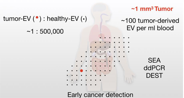
A mathematical-model was used to predict the concentration of tumor-derived EVs in circulation as a function of tumor size. Emerging single-EV technologies (SEA, DEST, ddPCR) are positioned to detect rare, tumor-EVs for the early discovery of small tumors (< 1 mm³) in humans.

INTRODUCTION

The only way to definitively cure aggressive cancers (e.g. pancreatic, lung) is to surgically resect them when they are still localized. For example, in pancreatic cancer, only 20% of patients will present with surgically resectable disease, while 40% will present with localized but surgically unresectable disease and 40% will present with metastatic disease. For those 20% of patients who were initially deemed surgically resectable, the 5 year cure rate has been a low 20%. If we are to cure more patients with cancer, new diagnostic tools are necessary to identify patients with preclinical and truly localized disease.

Technological advances have improved the capacity to detect circulating biomarkers in blood samples, including tumor-associated extracellular vesicle (EV, including exosomes and microvesicles)^[1], mutated or methylated cell-free DNA (cfDNA)^[2], metabolic parameters (e.g. onset of diabetes, muscle wasting)^[3], or combinations of these analytes ^[4]. Not all patients with localized tumors will have sufficient quantity of circulating cfDNA for detection and analysis, thus EV have emerged as a promising complementary method. We and others have developed a number of different analytical methods to analyze EV^[5–7]. Many of the earlier techniques relied on bulk measurements requiring ~ 10⁴-10⁶ EV for a single measurement. Yet, the identification of a small number of tumor-originating EV (such as those found in microscopic cancers) in a background of host EV may be impossible by bulk methods. One way to solve the problem is to develop single (“digital”) EV analysis techniques, which are now emerging^[8–11]. Armed with these technological advances key biological questions regarding the utility of EV as biomarkers can now be answered.

Most clinical EV studies have been conducted in advanced and metastatic disease. It is still unclear whether EV released by small tumors (<1 cm³) can indeed be detected by EV analysis in blood. A large number of factors influence the answer (e.g. tumor EV shed rates, clearance rates, concomitant host EV production) and which are often difficult to dissect experimentally. Conversely, in the mouse where genetically engineered models exist, the pharmacokinetics and mass laws are different (i.e. a 1 cm³ tumor in the mouse can be lethal whereas it is resectable in humans). To address these issues, we have been interested in modeling tumoral EV production and elimination. Using such an approach we were interested in predicting detection rates as well as the required diagnostic sensitivities and specificities of newly emerging EV tests and markers. Based on common pharmacological models and experimentally known literature values^[12] we present a computational model to address a number of interrelated variables such as the correlations between blood EV levels and tumor volume, EV levels and time of tumor progression, and circulating levels and pharmacokinetic parameters. We were particularly interested in addressing three main clinical questions: i) what are the circulating bulk EV (bEV) and tumor EV (tEV) levels as a function of tumor mass, ii) what are the different tumor sizes that would be detectable by different EV analytical techniques and iii) what are the diagnostic requirements for early cancer detection?

RESULTS

Model description and assumption

In mouse models of cancer, the number of circulating EV increases as tumors grow. For example, it has been shown in mice that tumors larger than 200 mm³ can increase total circulating bulk EV (bEV) by 5-fold^[13], whereas in humans some studies have shown increases by 1–2 orders of magnitude, or more^[14]. Several other parameters have been established experimentally and these form part of our modeling: i) the half-life of circulating EV is generally short (less than 5 minutes), but has a long terminal half-life in mice^[15]; ii) the small percent of EV that persist in circulation are likely due to EV partitioning into another compartment; iii) circulating EV are generally cleared by the liver, presumably by hepatic macrophages^[16,17]; and iv) while capillary beds of the liver are fenestrated and discontinuous allowing for EV intravasation, most organs have tight vasculature rendering them less permeable to EV uptake^[18,19]. Based on these experimental observations, we created a pharmacokinetic model (Figure 1; see formula in Methods). In essence, we divided the model into an EV production and an EV biodistribution/elimination part, each with sub-parameters. With respect to the latter we assumed primary liver distribution and elimination, with the potential of additional elimination routes, such as into urine and feces. To explain the persistence of some EV at later times resulting in the long terminal-half life observed in mice we also included a vascular endothelial binding component. To distinguish between bEV and tEV a baseline of healthy EV (hEV) was calculated, such that bEV = hEV + tEV. The production of tEV from the tumor was assumed to deposit the majority of tEV into circulation due to the leaky tumor vasculature and all EV in circulation were assumed to follow the same distribution and elimination patterns.

Figure 1: Overview.

The number of EVs in circulation available to assay is determined by the processes governing their distribution and elimination as well as their production. Tumors are assumed to produce EVs that are released into circulation that are then subject to vascular binding events and organ uptake. EVs are assumed to be predominately taken up by organs with fenestrated vasculature, such as the liver, where resident macrophages play a dominant role in eliminating them from circulation.

Modeling distribution and elimination

In order to model EV production and levels in circulation it is crucial to first have an understanding of the mechanisms that govern EV distribution and elimination. We thus set out to model the distribution of EV in mice. Figure 2 shows experimental data where B16 cell-line derived tEV were systemically administered into mice via the tail-vein injection^[20]. While the majority of dosed tEV disappear from circulation within the first ten minutes, some B16 tEV could still be detected in circulation up to 4 hours after being dosed. In line with expectations that organs with tight vasculature are impermeable to tEV extravasation, B16 tEV failed to accumulate to any appreciable extent in the majority of tissue (e.g. brain, heart, kidney, muscle, etc.). To maintain a robust model, a simplifying assumption that EV distribution is restricted to fenestrated organs (e.g. liver) was employed. In support of this assumption and in contrast to other tissues, liver showed rapid accumulation and retention of over 30% of the injected dose. While liver distribution and retention described the initial distribution phase well, it was not able to fit the long terminal half life observed. To improve fits and capture this critical observation, we hypothesized that some EV were able to persist in circulation due to a transient binding to vascular walls. To establish EV binding capacity to endothelial cells, human umbilical vein endothelial cells (HUVECs) were incubated with increasing doses of B16 tEV. This experiment illustrated that tEV show substantial binding to vascular cells in vitro (Supplementary Figure 1).

Figure 2: Distribution elimination model.

A. Systemically administered exogenous B16 EVs show rapid clearance from blood with concomitant rapid accumulation in the liver. Other organs (not shown) displayed minimal EV uptake (< 10% in total). Some B16 EVs were recovered in the urine and feces. A distribution and elimination model of ordinary differential equations depicted in figure 1 was used to fit (blue line) the experimental data (red dots) obtained from^[14]. The model fits described the data well across the collection period.

By incorporating a k_on and k_off to the vasculature for our EV distribution model we were able to fit the blood and liver data well both at early and later times (blood R² = 0.999, liver R² = 0.957). The estimated rapid association with the vasculature asserts that the majority of EV that disappear from circulation within the first 5 minutes are bound to the vascular walls. Since there was experimental data for urine and feces, we were additionally able to estimate the renal and fecal elimination rates. The other elimination pathway estimated was the hepatic elimination of EV that distribute into the liver. Specifically, the experimental data show the following parameters for EV distribution and elimination: T_1/2-⍺: 0.735 minutes; T_1/2-β: 87.6 minutes; Blood_%SS: 1.30%; Liver_%SS: 63.2%; Vascular-Wall_%SS: 35.5%; Hepatic-Clearance%: 90.04; Renal-Clearance%: 5.94; Fecal-Clearance%: 4.03 (Table 1).

Table 1:

Summary of experimental and theoretical parameters

	Parameter	Description	Species/Cancer	Estimate	(CV%) / [95% CI]	Notes
Distribution and Elimination Model	Vd-m	Volume of distribution [ml]	Mouse	1.53	Fix	Shah & Betts (2012) scaled to 25g mouse
	Vd-h	Volume of distribution [ml]	Human	6,004	Fix	Shah & Betts (2012) scaled to 75kg male
	t1/2	Blood half-life [min]	Mouse/Human	⍺: 0.735 β: 87.6	-	Calculated from Model
	RenalEXC	Renal Elimination [day−1]	Mouse/Human	1.932 × 10−2	(29.31)	Model Estimate
	FecalEXC	Fecal Elimination [day−1]	Mouse/Human	1.031 × 10−2	(16.00)	Model Estimate
	RESuptake	Hepatic Uptake [day−1]	Mouse/Human	0.3055	(5.516)	Model Estimate
	vascKon	Vasculature Kon [day−1]	Mouse/Human	0.6397	(5.418)	Model Estimate
	vascKoff	Vasculature Koff [day−1]	Mouse/Human	2.336 × 10−2	(18.18)	Model Estimate
	HepEli	Hepatic Elimination [day−1]	Mouse/Human	6.264 × 10−3	(7.961)	Model Estimate
Tumor Growth and tEV Production Model	kTgr	Tumor Growth Rate [day−1]	B16 MelanomaPeinado et al (2012)	0.1185	(8.4) / [0.0998 – 0.1393]	Gompertz Fit
	TumorMax	Max Tumor Volume [ml]		2,590	(14.8) / [1,979 – 3,669]	Gompertz Fit
	ktEV-SHED	Shed Rate of Tumor EVs [day−1]		6.522 × 10−2	(21.81)	Model Estimate
	kTgr	Tumor Growth Rate [day−1]	PYMT BreastSharma et al (2017)	0.1724	(14.5) / [0.1307 – 0.2365]	Malthusian Fit
	TumorMax	Max Tumor Volume [ml]		N/A	-	-
	ktEV-SHED	Shed Rate of Tumor EVs [day−1]		4.010	(17.76)	Model Estimate
	kTgr	Tumor Growth Rate [day−1]	KPC PancreaticSharma et al (2017)	1.424 × 10−2	(7.1) / [0.0072 – 0.0229]	Gompertz Fit
	TumorMax	Max Tumor Volume [ml]		477.3	(7.6) / [401.0 – 673.8]	Gompertz Fit
	ktEV-SHED	Shed Rate of Tumor EVs [day−1)		0.2208	(5.399)	Model Estimate
	kTgr	Tumor Growth Rate [day−1]	KIC PancreaticSharma et al (2017)	7.852 × 10−2	(13.9) / [0.0615 – 0.1133]	Gompertz Fit
	TumorMax	Max Tumor Volume [ml]		2081	(15.9) / [1,546 – 2,973]	Gompertz Fit
	ktEV-SHED	Shed Rate of Tumor EVs [day−1]		4.954 × 10−2	(13.49)	Model Estimate

EV production rate is largely constant over the tumor life-time

Having established a generic mathematical model for EV distribution and elimination, we next analyzed bEV levels as a function of tumor volumes. This is important since different cancers grow at different rates, and thus will produce and shed tEV differently into circulation. We identified experimental data from four murine cancer models where tumor volumes and serial bEV values had been published: i) B16 melanoma model^[14], ii) PYMT breast cancer^[13], iii) Kras^G12d/P53^−/− (KPC) pancreatic cancer^[13] and iv) KIC pancreatic cancer models^[13]. In order to estimate bEV in circulation, it was first necessary to find a suitable model of tumor growth for these data. B16, KPC, and KIC tumor models were well described by a Gompertz growth function that estimates an exponential tumor growth rate and a self-limiting tumor-volume maximum (B16 R² = 0.998, KPC R² = 0.976, KIC R² = 0.982) while PYMT was best described by simple Malthusian (exponential only) growth (R² = 0.998), although it also fit well with a Gompertz growth function (Figure 3a). PYMT tumors showed the most aggressive growth rate with a doubling time of 4.0 days. B16 xenografts showed a doubling time of 8.4 days whereas the doubling times of KIC tumors was 12.7 days and the doubling time of KPC tumors was estimated to be 48.5 days (Figure 3a).

Figure 3: Production model.

A) Tumor growth for four preclinical mouse models of cancer, KIC (Pancreatic Ductal Adenocarcinoma)^[13], KPC (Pancreatic Ductal Adenocarcinoma)^[13], B16 (metastatic melanoma)^[14], and PYMT (ER- Breast Cancer)^[13], were fit to either a Gompertz or Malthusian growth model. B) The tumor growth parameters (from A) and the previously estimated distribution and elimination parameters were fixed and tEV-SHED rates and hEV baselines were estimated to fit the total bEVs in circulation. C) The total tEV in circulation is shown by subtracting the baseline of hEV. Error bars / shaded regions depict observed / model-generated standard deviation.

Having described the tumor volumes, we next sought a mathematical relationship to describe bEV production over time as a function of tumor size assuming hEV levels remain constant. The initial assumption was that tEV were shed from tumors at an intrinsic rate set by the unit cell, and therefore tumor volume and increases in circulating bEV would be correlated. For time-matched experimental bEV concentrations and tumor volume data a high degree of correlation over the tumor lifetime was observed for KIC (R²=0.99), KPC (R²=0.99), and B16 (R²=0.98). The PYMT data showed high correlation for tumors smaller than 20 mm³ (R²=0.98) with evidence of a lower tEV production rate at later times (overall R²=0.53). Seeking a generalizable model, we fit all four datasets using a time-invariant first-order shed rate parameter. The cancer-type specific k_tEV-Shed parameter fit the data satisfactorily (KIC R² = 0.727, B16 R² = 0.853, KPC R² = 0.917, and PYMT R² = 0.632) for all four cancer models (Figure 3b). Among these cancer types, we witnessed a 81 fold range in shed rates. Interestingly, tumor aggressiveness as gauged by growth rate did not necessarily correlate with tEV shedding. While B16 and KIC tumors were fast growing and reached a larger volume, they had the lowest rate of tEV shedding (0.06522 and 0.04954 day⁻¹ respectively). The tEV shed rate estimated for the slower growing KPC tumors was significantly higher (0.2233 day⁻¹). Even though KPC tumors remained much smaller than B16 or KIC tumors, similar increases in circulating bEV were observed, indicative of a higher tEV shed rate. The fastest growing tumor, PYMT, did have the highest tEV shed rate (4.010 day⁻¹).

EV in circulation as a function of tumor volume in mouse and humans

The modeling indicates that each 1 mm³ of tumor volume in mice results in 4.0 × 10⁴ to 3.7 × 10⁶ tEV per ml blood for low to high tEV-shedding (Figure 4a). Based on this observed range of tEV shed rates, we next modeled tEV levels in human cancers. We made the following assumptions: i) parameters that govern the distribution and elimination of EV in mice can be extrapolated to humans; ii) the physiologic volume of distribution (total blood volume) in humans is ~4,000 fold greater than in mice; and iii) that human tumors grow at a slower rate of k_Tgr = 0.023 day⁻¹ (30 day doubling time) and to a larger volume with a maximum of 1,500 cm³. Our first assumption is supported by observations that the kinetics of lipid nanoparticles cleared by the reticuloendothelial (RES) / mononuclear phagocyte (MPS) system are relatively conserved between mice and humans ^[21]. The second assumption is well documented in the literature^[12] and accounts for the simple “dilution effect” of tEV into a larger circulation volume. The third assumption is based on scaling the average maximum tumor volume in mice to humans by body weight, however, provided the parameter estimate is kept reasonably large, small tumors in humans still track closely to exponential growth. The resulting simulation from these assumptions demonstrates that for humans, each 1 mm³ of tumor volume would add 23 tEV per ml blood for low-shed rate tumors to up to 1900 tEV per ml of blood for high-shed rate tumors (Figure 4b). Since tEV shed rates were simulated from the mouse data, the decreased slope of tEV per mm³ of tumor volume in humans is mostly attributable to the larger distribution volume of blood in humans compared to mice.

Figure 4: Predicting human tEV from mouse data.

A) The relationship between tumor volume and tEV in circulation from the EV production and distribution / elimination model is shown for the four preclinical mouse cancer types^[13,14]. Higher tEV shed rates result in a steeper relationship. Shaded region represents the 95% confidence interval for the tEV shed rate estimate. B) The model was adapted for human predictions by scaling tumor growth parameters, blood volume, and simulating the observed range of tEV shed rates. Note, x-axis for mice is mm³ and for humans is cm³.

Comparing model predictions to human clinical data

Considering we witnessed a greater than 80-fold range in EV shed rates for the four preclinical mouse models of cancer available, it is likely that actual EV shedding across the spectrum of human cancers may span an even larger range. In order to simulate expected increases in total EV, a 2-fold higher EV shed rate and 2-fold lower shed rate than the highest and lowest observed shed rates were included (gray region). The mean of the observed shed rates was simulated as the best estimation of expected fold increases in circulating EV as a function of a growing tumor (Figure 5a).

Figure 5: Predictions in humans / detection comparison.

A) The increase in total circulating bEVs in humans as a function of tumor burden is presented in fold-changes over the baseline of hEV, the mean of the observed shed rates expanded by two-fold in mouse tumors is depicted as a blue line while the highest and lowest shed rate observed in mouse models is depicted by the gray shaded region. B) Model predicted fold-increases in bEV were compared to available clinical data. The model correlated well with clinical data from three different cancer types (R²=0.956, blue dashed line. Black dashed line represents the line of identity). C) The range of tEV predicted from the observed shed rates as a function of tumor volume for humans is plotted in gray, while the geometric mean is plotted as a blue line. Reported detection limits of different EV analytical assays are shown along with the theoretical size-limits of detectable tumor. D) Since not all tEV may be differentiable from hEV, a range of ‘cancer marker’ percent-positive tEV graph is shown. For example, if only 1% of tEV have a chosen ‘cancer marker’ or marker panel, then single-EV analytical assays could still in theory be deployed to detect cancer as small as 0.001 cm³ (white arrows).

As can be seen, appreciable percentage increases in total circulating EV is not expected until tumors are already quite large (> 50 cm³, about the size of a golfball). In advanced disease however, many patients present with tumors of several cm³ up to 1,000 cm³ or even more, especially when metastatic sites are considered and summated. Therefore, the model does predict that these patients would indeed have fold-level increases in circulating EV, as has been reported^[22]. In order to validate the model for predicting increases in circulating EV in later-stage human cancers we identified three studies^[23–25] where increases in circulating EV were reported alongside tumor volumes or with cancer staging that allowed for inferred tumor volumes. The model-calculated fold increases in circulating EV was well matched to observed fold increases (Figure 5b R²=0.929). These observations indicate that the model is indeed accurate in predicting EV levels in clinical samples.

Detection of small human tumors by tEV analysis

What are the different tumor sizes that would be detectable by different EV analytical techniques? To answer this question we applied the model to predict thresholds of tumor detection for various EV-detection assays. According to literature reports and our own experience, bulk methods such as ELISA, or Western Blot, often require at a minimum ~ 10⁴-10⁶ EV per sample to reliably detect abundant EV markers^[5]. For the highest EV-shedding tumors, these methods might capture tumors as small as ~1 cm³. However, the mean EV shed rate observed predicts that bulk methods would be more suited toward assaying larger tumors (~10 cm³) such as for therapy monitoring. To detect small tumors, more sensitive assays are required. These include approaches such as μNMR, iMER, iMEX, nPLEX, among others, that have achieved orders of magnitude higher sensitivity over traditional approaches^[5]. For a typical tumor, all of these approaches are predicted to be able to detect lesions smaller than 1 cm³ (Figure 5c). For single-EV resolution or near-single-EV resolution assays such as SEA^[8], DEST^[26], or ddPCR^[11] it may even be possible to detect tumors as small as 1×10⁻⁵ cm³ (10 microgram, or about 10,000 tumor cells). The challenge however is to find EV biomarkers (or combinations, i.e. “signatures”) that can distinguish tEV unequivocally from other host cell EV based on molecular markers.

To model the different scenarios of tEV detectability, we plotted tumor volume against different levels of tEV specificity (i.e. from 100% of tEV containing a unique and detectable ‘cancer marker’ down to only 1 in 10,000 tEV carrying a unique marker) (Figure 5d). While no actual data exists on what these percentages are in human samples, we expect that only 0.1–10% of tEV actually carry unique markers that would allow them to be differentiated from host cells. Based on current technical feasibilities (e.g. multiplexed SEA) and assuming 1% of tEV are distinguishable from hEV, we estimate human cancer detection ranges in the order of 0.1 mm³ for high-tEV-shedding or 7 mm³ for low-tEV-shedding tumors.

Single EV Analysis opens a window to earlier cancer detection

Our next application of the model was to illustrate how different tEV detection assays are positioned to detect tumors earlier given typical tumor growth rates in humans. A slow growing tumor that doubles in volume every year, and a tumor that grows at a 10x faster rate (doubling nearly every month) were simulated. Since most clinical data suggested a higher-end shed rate we used 1.0 day⁻¹ as the k_tEV-SHED parameter value. For typical tumors growing at a moderately aggressive ~1-month doubling rate, the model predicts that bulk methods would not open any windows to earlier cancer detection. More sensitive methods however, should be able to detect tEV within the first 3 years of tumor growth, nearly three years before the tumor reaches a size of 1 cm³ and would thus be readily detectable by medical imaging (Figure 6). Since many cancers grow slowly, and have likely been growing undetectable for several years or decades before detection, we also simulated a tumor growing at a yearly doubling rate. For such slow-growing tumors, single-EV analysis assays are predicted to detect cancer over 3-decades before they could be easily identified by imaging.

Figure 6: Time window of tEV detection.

A) For tumors that double every month and shed tEV at the higher end of observed rates aligning with human clinical data, the model predicts that after ~2 years of tumor growth there will be ~100 tEV per ml, a number that should be detectable by single-EV imaging even if only 1% of tEV are positive for a chosen marker. This is ~3-years before the tumor would reach a size of 1 cm³ and be readily detected by imaging. B) Many human tumors grow much slower. For tumors that double every year, the model predicts that tumors could be detected early in the third decade of growth, still decades before reaching a size readily caught by imaging.

DISCUSSION

We have developed a mathematical framework to predict ranges of EV during cancer development and progression as has been done for other blood-based biomarkers^[27–29]. The main motivation for developing the mathematical foundation was to create a working model in which the effects of physiological variations on EV levels could be predicted. This in turn would help interpretation of the divergent literature, sometimes absent clinical data, the non-reproducibility of some EV molecular markers in clinical trials and necessary requirements for next generation EV diagnostics.

Based on preclinical murine data in melanoma, breast and pancreatic cancer, we first developed a model of EV production and merged it with biodistribution and elimination principles. Since the developed model fit the experimental mouse data well, we then extrapolated the model to predict human EV levels. Similarly, the model predictions aligned well with available clinical data in advanced cancers^[24,25,30]. Divergences in model predictions are most likely a result of a few limitations and other considerations unaccounted for. First, the model currently does not include circadian variations in biomarker shedding, as may be expected in tumors or other organs, because these fluctuations have not been adequately studied to date. Second, the tumor burden volume reported here represents the total number of biomarker-shedding primary and metastatic cells. Lastly, the model does not account for different shedding rates or growth rates in primary and metastatic tumor cell, or for the possibility that tumor EV shed rates could vary over time. Irrespective of these limitations, we were particularly interested in three questions: i) what are the circulating tEV and bEV levels as a function of tumor mass, ii) what are the different tumor sizes that would be detectable by different EV analytical techniques and iii) what are the diagnostic requirements for early cancer detection?

Relationship between tumor size, bEV and tEV

EV are shed by a variety of host and tumor cells and circulating EV levels are invariably a combination of both. In healthy individuals, conservative estimates of bEV levels are at least 10⁷⁻⁸ per mL of blood ^[31] but in cancer patients these numbers can increase to > 10⁹ per mL in advanced stages^[32]. These higher levels of bEV are likely a combination of tEV, as well as EV shed by inflammatory cells associated with cancer (iEV) and drifts in baseline levels of EV. Reports that cancer cells shed EV markedly more than healthy cells ^[33,34], and observations that cancer patients have elevated levels of circulating EV has positioned EV as a prime candidate for liquid biopsy and cancer diagnosis strategies. However, there are no longitudinal studies able to link tumor size to increases in circulating tEV in humans.

By modeling tumor growth with increases in circulating bEV in preclinical mouse models of cancer we were able to predict the relationship between tumor size and circulating bEV in humans. The data supported linear first-order distribution and elimination processes across the observed range. This allowed us to capture the amount of circulating bEV as a function of tumor volume well for four different preclinical cancer models by simply using a single first-order EV shed rate. In humans, each 1 mm³ increase in tumor volume is predicted to correspond to an increase in circulating bEV of ~23 to 1,900 EV per ml. Therefore, each cm³ increase in tumor volume is expected to increase the baseline of circulating bEV in a human patient by ~1% (0.07 to 2.5%). By steady state considerations, assuming the level of EV in circulation is 4.2 × 10⁷ per ml and the cellular volume of healthy tissue is 5.4 × 10⁷ mm³, then healthy tissue corresponds to ~0.78 hEV per ml per mm³. This means our model predicts cancer cells shed tEV at about ~40 – 1,200 times the rate of healthy cells, which fits well with what has been reported in vitro and in vivo ^[34].

While the primary goal of the current study was to look at blood levels of EV, a notable take-away from these modeling efforts was that the fecal and renal elimination routes should not be overlooked. Due to the concentrating effect of both renal and fecal elimination, both urine and feces could easily contain EV concentrations approaching or exceeding EV concentrations in blood. At steady state, assuming an adult human urinated 1,000 ml and excreted 500 g of feces per day, the concentration of EVs would be 1.06-fold higher per milliliter urine and 1.44-fold higher per gram feces than the blood concentration per milliliter. In support of this, reports have shown EV concentrations in urine on the order of 10⁸ to 10^{10 [35]}. However, It is unclear if the tEV biomarkers are transformed by these elimination processes.

The presence of uniquely identifying molecular markers on tEV is critical to detect and differentiate tEV from host cell EV. As the ability to measure specific tEV by the use of molecular markers increases, diagnostic accuracy of tests would undoubtedly increase. A number of tEV “specific” biomarkers and signatures have been described relying on protein^[36] or RNA signatures^[37–39]. For example it has been shown that colorectal cancer EV contain EGFR, EpCAM, CD24 and GPA33, pancreatic cancer contain EGFR, EPCAM, WNT2, MUC1^[1] and glioblastoma contain IDH1132, EGFRv3^[8]. New biomarkers are constantly being described and the question of which ones are best markers and marker combinations remains to be answered. It is becoming clear however, that a single biomarker alone may not be able of detecting tEV with sufficient sensitivity and specificity.

Diagnostic capabilities of established EV analytical techniques

A number of EV diagnostic techniques are commonly available. Total bEV concentration in blood can be readily measured by nanoparticle tracking analysis (NTA)^[40], resistive pulse sensing ^[41], flow cytometry^[42] among others. However, due to the large variability in bEV baselines across healthy individuals and the observation that low-EV-shedding tumors would not appreciably increase the total concentration of bEVs (tEV << hEVs), these strategies are unlikely to be helpful in detecting cancer. Therefore, tEV analysis is usually based on the measurement of specific molecular markers. Our team has developed a series of technologies to quantify and assay tEV in blood samples^[5]. These technologies differ in i) detection sensitivity, ii) throughput capability, iii) ability to differentiate hEV or tEV via molecular markers and iv) cost. Specific examples of new technologies include nanoplasmonics^[33], μNMR^[43,44], acoustics^[45], magneto electrochemical sensing^[46], and bead-based analyses^[47]. These technologies often play different/complementary roles in biological research and in clinical applications (e.g. longitudinal treatment monitoring; early detection). For example, in a research setting lower throughput/higher sensitivity methods may be preferred, whereas in a clinical setting throughput, sensitivity/specificity and cost do matter. Figure 5c summarizes the diagnostic sensitivities of some of these technologies and predicts what tumor sizes would be detectable with each of them. It is of particular interest to point out that both IMEX (electrochemical sensing; fast and inexpensive) and nPLEX (plasmonic sensing) are both theoretically capable of detecting cancers ~ 0.1 cm³ in size.

Diagnostic requirements for early cancer detection

It is predicted that emerging single EV analytical techniques will further increase the detection sensitivity of tEV. A number of single EV analytical methods have been proposed. These include analysis by microscopic imaging of immobilized vesicles (SEA)^[8,9], modified flow cytometry^[8,48–51], and digital ELISA^[26]. Finally, a new method for ultra-sensitive protein based single EV analysis is immuno digital droplet polymerase chain reaction (iddPCR) described in a companion article in this issue^[11]. Using these approaches it should be possible to detect human cancers as small as 0.01 mm³.

MATERIALS AND METHODS

Data sources

Physiological volumes were obtained from^[12]. B16 pharmacokinetic and distribution data was obtained from ^[20]. Levels of bEVs for KIC, KPC, and PYMT cancer models as well as corresponding tumor size for PYMT tumors was obtained from^[13]. For KPC, tumor volume data was obtained from^[52] and KIC tumor volume was obtained from^[53]. B16 bEV levels and tumor volumes were obtained from^[14].

For clinical validation in ovarian cancer, the tumor volume used was the average tumor size upon diagnosis of stage III and IV patients reported by Horvath et al^[54] and increases in circulating bEVs was obtained from^[23]. For liver cancer, the tumor volumes and bEVs were reported in text ^[25]. For colorectal cancer, tumor volumes and corresponding EV levels were provided by the study authors^[24].

Data Handling

All data was obtained directly from the study authors or through digitation of primary figures (PlotDigitizer 2.6.8). For modeling the tumor growth dynamics in units of mm³ the assumption that each mm³ contains 1 × 10⁶ cells was employed. With this understanding B16 initial tumor volume was fixed to 1.0 since 1 × 10⁶ cells were initially implanted. For KIC, constraining the initial tumor volume to a minimum of 1 × 10⁻⁶ (one cell) improved parameter estimation of tumor growth rate and maximum volume even with the sparse data. For linking the EV production model to the raw data reported by Sharma et al. tEV in circulation were converted from reported units to EV numbers per ml by the following transformations: first, the picogram exposed phosphatidylethanolamine (PE) was converted to molecular units via PE molecular weight (692 g mol⁻¹) and then to EV numbers by assuming mol% of EV lipid was 5% ^[55] and that a representative 100 nm EV contains 8 ×10⁴ lipid molecules. Phosphatidylserine-positive (PS+) EVs were scaled to total EVs by assuming 66.5% of spherical blood EVs are PS+ ^[31]. To validate model predictions with observed human clinical tEV increases it was necessary to normalize the data to facilitate meaningful comparisons. Due to disparate EV isolation and quantification methods, numbers of EV per ml in human blood is routinely reported in a range of 10⁷ to 10¹² EVs per ml ^[42], with the higher end estimations almost certainly resulting from co-contaminating lipid particles or protein aggregates. While 10⁹ is a uniformly accepted baseline of healthy EV numbers per ml, here we used the ~20-fold more conservative value 4.2 × 10⁷ since this number was established from a well-validated total-capture electron microscopy method devoid of many of the problematic biases introduced by other enumeration methods such as NTA or flow cytometry ^[31]. The reported baseline of healthy volunteer data was normalized to this value and patient EV numbers were normalized by the same factor to make EV-number to EV-number comparisons. Alternately, model validation with human clinical data was performed by comparing predicted fold-changes in EVs with observed fold-changes in EVs of cancer patients over the within-study healthy controls. For the individual level data available for colorectal cancer patients, a binning approach followed by outlier test was conducted to correct for a small number of small-tumor patients with very high EV concentrations.

Model

Equations 1 – 5 describe tEV distribution and elimination in mass units where: vasc_kon is the first order rate constant describing association of tEV to the vascular walls, vasc_koff is the first order rate constant describing dissociation of tEV from the vascular walls back into circulation, Renal_EXC and Fecal_EXC are the first order rate constants of tEV eliminated into urine and feces, respectively, RES_uptake is the first order rate constant of hepatic uptake, and Hep_Eli is the first order rate constant of tEV eliminated in the liver (days⁻¹).

Equation 6 describes the tumor growth dynamics and production of tEV. k_Tgr is the first order growth rate of the tumor (days⁻¹) and Tumor_Max is the maximum tumor volume (mm³). Under the case where a tumor is present, tEV input from equation 6 is modeled in equation 1 by the first order tumor-EV shed rate: k_tEVSHED (days⁻¹). For PYMT tumor growth, the log term was omitted allowing for uninhibited Malthusian growth.

$$\frac{d\text{tEV}}{dt}=-\left({vasc}_{Kon}\times \text{tEV}\right)-\left({Renal}_{EXC}\times \text{tEV}\right)-\left({Fecal}_{EXC}\times \text{tEV}\right)-\left(RE{S}_{uptake}\times \text{tEV}\right)+\left({vasc}_{Koff}\times \text{VASC}\right)+\left(\text{ TUMOR }\times ktE{V}_{SHED}\right)$$ Eq. 1,

Tumor EVs in circulation:

Tumor EVs bound to vasculature:

$$\frac{d\text{ VASC }}{dt}=\left(vas{c}_{Kon}\times \text{tEV}\right)-\left(vas{c}_{Koff}\times \text{VASC}\right)$$ Eq. 2,

Tumor EVs cleared by the liver:

$$\frac{d\text{ LIVER }}{dt}=\left(\text{tEV}\times RE{S}_{uptake}\right)-\left(\text{LIVER}\times He{p}_{Eli}\right)$$ Eq. 3,

Tumor EVs cleared renally:

$$\frac{d\text{ URINE }}{dt}=\left(\text{tEV}\times Rena{l}_{EXC}\right)$$ Eq. 4,

Tumor EVs cleared fecally:

$$\frac{d\text{ FECES }}{dt}=\left(\mathrm{tEV}\times Feca{l}_{EXC}\right)$$ Eq. 5,

Tumor volume:

$$\frac{d\text{TUMOR}}{dt}=k_{Tgr}\times \log \left(\frac{Tu{mor}_{Max}}{\text{TUMOR}}\right)\times \text{TUMOR}$$ Eq. 6,

Model Fitting

Model fitting was performed in consecutive stages. First, distribution and elimination model parameters were estimated using the maximum likelihood algorithm with ADAPT v5. In parallel, tumor growth rates and maximums were estimated using the Gompertz (B16, KIC, KPC) or Malthusian (PYMT) functions built within Graphpad Prism v8. The parameter values from these steps were then fixed to estimate the hEV baseline, and k_tEV-Shed rate parameters for the tEV production model also within ADAPT using the maximum likelihood algorithm. The variance model was: V_i = (intercept + slope · Y (t_i))² where V_i is the variance of the response at the ith time point, t_i is the actual time at the ith time point, and Y(t_i) is the predicted response at time t_i from the model. Variance parameters intercept and slope were estimated together with system parameters. Model performance was evaluated by goodness-of-fits, visual inspection, sum of square residuals, Akaike Information Criterion, and Coefficient of Variation (CV) of the estimated parameters.

Statistical Analysis

Pre-processing of data was performed as described in ‘Data Handling’. All data are presented as mean ± S.D. or 95% confidence interval as indicated in the figure legend. For each experiment sample size (n) is determined by the corresponding original report and no additional statistical tests have been run. Model suitability for tumor growth kinetics was performed within Graphpad Prism 8.2.1. All tumor growth models passed the the “Replicates test for lack of fit” (p = 0.9946 PYMT, p = 0.6330 KPC, p = 0.9620 B16, p = 0.4397 KIC, evaluated at ⍺ 0.05).

REFERENCES

- [1].Yang KS, Im H, Hong S, Pergolini I, Del Castillo AF, Wang R, Clardy S, Huang CH, Pille C, Ferrone S, Yang R, Castro CM, Lee H, Del Castillo CF,Weissleder R. Sci Transl Med 2017, 9, [DOI] [PMC free article] [PubMed] [Google Scholar]
- [2].Bettegowda C, Sausen M, Leary RJ, Kinde I, Wang Y, Agrawal N, Bartlett BR, Wang H, Luber B, Alani RM, Antonarakis ES, Azad NS, Bardelli A, Brem H, Cameron JL, Lee CC, Fecher LA, Gallia GL, Gibbs P, Le D, Giuntoli RL, Goggins M, Hogarty MD, Holdhoff M, Hong SM, Jiao Y, Juhl HH, Kim JJ, Siravegna G, Laheru DA, Lauricella C, Lim M, Lipson EJ, Marie SK, Netto GJ, Oliner KS, Olivi A, Olsson L, Riggins GJ, Sartore-Bianchi A, Schmidt K, Shih LM, Oba-Shinjo SM, Siena S, Theodorescu D, Tie J, Harkins TT, Veronese S, Wang TL, Weingart JD, Wolfgang CL, Wood LD, Xing D, Hruban RH, Wu J, Allen PJ, Schmidt CM, Choti MA, Velculescu VE, Kinzler KW, Vogelstein B, Papadopoulos N,Diaz LA. Sci Transl Med 2014, 6, 224ra24. [Google Scholar]
- [3].Yuan C, Clish CB, Wu C, Mayers JR, Kraft P, Townsend MK, Zhang M, Tworoger SS, Bao Y, Qian ZR, Rubinson DA, Ng K, Giovannucci EL, Ogino S, Stampfer MJ, Gaziano JM, Ma J, Sesso HD, Anderson GL, Cochrane BB, Manson JE, Torrence ME, Kimmelman AC, Amundadottir LT, Vander Heiden MG, Fuchs CS,Wolpin BM. J Natl Cancer Inst 2016, 108, djv409. [DOI] [PMC free article] [PubMed] [Google Scholar]
- [4].Cohen JD, Li L, Wang Y, Thoburn C, Afsari B, Danilova L, Douville C, Javed AA, Wong F, Mattox A, Hruban RH, Wolfgang CL, Goggins MG, Dal Molin M, Wang TL, Roden R, Klein AP, Ptak J, Dobbyn L, Schaefer J, Silliman N, Popoli M, Vogelstein JT, Browne JD, Schoen RE, Brand RE, Tie J, Gibbs P, Wong HL, Mansfield AS, Jen J, Hanash SM, Falconi M, Allen PJ, Zhou S, Bettegowda C, Diaz LA, Tomasetti C, Kinzler KW, Vogelstein B, Lennon AM,Papadopoulos N. Science 2018, 359, 926. [DOI] [PMC free article] [PubMed] [Google Scholar]
- [5].Shao H, Im H, Castro CM, Breakefield X, Weissleder R,Lee H. Chem Rev 2018, 118, 1917. [DOI] [PMC free article] [PubMed] [Google Scholar]
- [6].Im H, Lee K, Weissleder R, Lee H,Castro CM. Lab Chip 2017, 17, 2892. [DOI] [PMC free article] [PubMed] [Google Scholar]
- [7].Im H, Shao H, Weissleder R, Castro CM,Lee H. Expert Rev Mol Diagn 2015, 15, 725. [DOI] [PMC free article] [PubMed] [Google Scholar]
- [8].Lee K, Fraser K, Ghaddar B, Yang K, Kim E, Balaj L, Chiocca EA, Breakefield XO, Lee H,Weissleder R. ACS nano 2018, 12, 494. [DOI] [PMC free article] [PubMed] [Google Scholar]
- [9].Fraser K, Jo A, Giedt J, Vinegoni C, Yang KS, Peruzzi P, Chiocca EA, Breakefield XO, Lee H,Weissleder R. Neuro Oncol 2018, [DOI] [PMC free article] [PubMed] [Google Scholar]
- [10].Ko J, Wang Y, Gungabeesoon J, Pittet M, Weitz D,Weissleder R (2019). Droplet-based single EV sequencing for rare immune subtype discovery. Proceedings from μ-TAS 2019. [Google Scholar]
- [11].Ko J, Wang Y, Carlson JC, Marquard A, Gungabeesoon J, Charest A, Weitz D, Pittet M,Weissleder R. Adv Biosystems 2020, in press. [DOI] [PMC free article] [PubMed] [Google Scholar]
- [12].Shah DK,Betts AM. J Pharmacokinet Pharmacodyn 2012, 39, 67. [DOI] [PubMed] [Google Scholar]
- [13].Sharma R, Huang X, Brekken RA,Schroit AJ. British journal of cancer 2017, 117, 545. [DOI] [PMC free article] [PubMed] [Google Scholar]
- [14].Peinado H, Alečković M, Lavotshkin S, Matei I, Costa-Silva B, Moreno-Bueno G, Hergueta-Redondo M, Williams C, García-Santos G,Ghajar CM. Nature medicine 2012, 18, 883. [DOI] [PMC free article] [PubMed] [Google Scholar]
- [15].Morishita M, Takahashi Y, Nishikawa M,Takakura Y. J Pharm Sci 2017, 106, 2265. [DOI] [PubMed] [Google Scholar]
- [16].Charoenviriyakul C, Takahashi Y, Morishita M, Matsumoto A, Nishikawa M,Takakura Y. Eur J Pharm Sci 2017, 96, 316. [DOI] [PubMed] [Google Scholar]
- [17].Imai T, Takahashi Y, Nishikawa M, Kato K, Morishita M, Yamashita T, Matsumoto A, Charoenviriyakul C,Takakura Y. J Extracell Vesicles 2015, 4, 26238. [DOI] [PMC free article] [PubMed] [Google Scholar]
- [18].Wisse E, Jacobs F, Topal B, Frederik P,De Geest B. Gene Ther 2008, 15, 1193. [DOI] [PubMed] [Google Scholar]
- [19].Sarin H. J Angiogenes Res 2010, 2, 14. [DOI] [PMC free article] [PubMed] [Google Scholar]
- [20].Morishita M, Takahashi Y, Nishikawa M, Sano K, Kato K, Yamashita T, Imai T, Saji H,Takakura Y. J Pharm Sci 2015, 104, 705. [DOI] [PubMed] [Google Scholar]
- [21].Gabizon A, Shmeeda H,Barenholz Y. Clin Pharmacokinet 2003, 42, 419. [DOI] [PubMed] [Google Scholar]
- [22].Logozzi M, De Milito A, Lugini L, Borghi M, Calabrò L, Spada M, Perdicchio M, Marino ML, Federici C, Iessi E, Brambilla D, Venturi G, Lozupone F, Santinami M, Huber V, Maio M, Rivoltini L,Fais S. PLoS One 2009, 4, e5219. [DOI] [PMC free article] [PubMed] [Google Scholar]
- [23].Schwich E, Rebmann V, Horn PA, Celik AA, Bade-Döding C, Kimmig R, Kasimir-Bauer S,Buderath P. Cancers (Basel) 2019, 11, [DOI] [PMC free article] [PubMed] [Google Scholar]
- [24].Tian Y, Ma L, Gong M, Su G, Zhu S, Zhang W, Wang S, Li Z, Chen C, Li L, Wu L,Yan X. ACS Nano 2018, 12, 671. [DOI] [PubMed] [Google Scholar]
- [25].Julich-Haertel H, Urban SK, Krawczyk M, Willms A, Jankowski K, Patkowski W, Kruk B, Krasnodębski M, Ligocka J, Schwab R, Richardsen I, Schaaf S, Klein A, Gehlert S, Sänger H, Casper M, Banales JM, Schuppan D, Milkiewicz P, Lammert F, Krawczyk M, Lukacs-Kornek V,Kornek M. J Hepatol 2017, 67, 282. [DOI] [PubMed] [Google Scholar]
- [26].Yang KS, Ciprnai D, Oshea A, Fletcher-Mercaldo S, Mino-Kenudson M, Fernadez C,Weissleder R. Sci Transl Med 2020, in review. [Google Scholar]
- [27].Hori SS,Gambhir SS. Sci Transl Med 2011, 3, 109ra116. [DOI] [PMC free article] [PubMed] [Google Scholar]
- [28].Hazelton WD,Luebeck EG. Sci Transl Med 2011, 3, 109fs9. [DOI] [PMC free article] [PubMed] [Google Scholar]
- [29].Eftimie R,Hassanein E. Journal of translational medicine 2018, 16, 73. [DOI] [PMC free article] [PubMed] [Google Scholar]
- [30].Schwich E, Rebmann V, Horn PA, Celik AA, Bade-Döding C, Kimmig R, Kasimir-Bauer S,Buderath P. Cancers (Basel) 2019, 11, [DOI] [PMC free article] [PubMed] [Google Scholar]
- [31].Arraud N, Linares R, Tan S, Gounou C, Pasquet JM, Mornet S,Brisson AR. J Thromb Haemost 2014, 12, 614. [DOI] [PubMed] [Google Scholar]
- [32].König L, Kasimir-Bauer S, Bittner AK, Hoffmann O, Wagner B, Santos Manvailer LF, Kimmig R, Horn PA,Rebmann V. Oncoimmunology 2017, 7, e1376153. [DOI] [PMC free article] [PubMed] [Google Scholar]
- [33].Whiteside TL. Adv Clin Chem 2016, 74, 103. [DOI] [PMC free article] [PubMed] [Google Scholar]
- [34].Ferguson SW, Megna JS,Nguyen J (2018). Composition, Physicochemical and Biological Properties of Exosomes Secreted From Cancer Cells In Diagnostic and Therapeutic Applications of Exosomes in Cancer (pp. 27–57). Elsevier. [Google Scholar]
- [35].Vogel R, Coumans FA, Maltesen RG, Böing AN, Bonnington KE, Broekman ML, Broom MF, Buzás EI, Christiansen G, Hajji N, Kristensen SR, Kuehn MJ, Lund SM, Maas SL, Nieuwland R, Osteikoetxea X, Schnoor R, Scicluna BJ, Shambrook M, de Vrij J, Mann SI, Hill AF,Pedersen S. J Extracell Vesicles 2016, 5, 31242. [DOI] [PMC free article] [PubMed] [Google Scholar]
- [36].Im H, Shao H, Park YI, Peterson VM, Castro CM, Weissleder R,Lee H. Nat Biotechnol 2014, 32, 490. [DOI] [PMC free article] [PubMed] [Google Scholar]
- [37].Skog J, Würdinger T, van Rijn S, Meijer DH, Gainche L, Sena-Esteves M, Curry WT, Carter BS, Krichevsky AM,Breakefield XO. Nat Cell Biol 2008, 10, 1470. [DOI] [PMC free article] [PubMed] [Google Scholar]
- [38].Ebrahimkhani S, Vafaee F, Hallal S, Wei H, Lee MYT, Young PE, Satgunaseelan L, Beadnall H, Barnett MH, Shivalingam B, Suter CM, Buckland ME,Kaufman KL. NPJ Precis Oncol 2018, 2, 28. [DOI] [PMC free article] [PubMed] [Google Scholar]
- [39].Lai X, Wang M, McElyea SD, Sherman S, House M,Korc M. Cancer Lett 2017, 393, 86. [DOI] [PMC free article] [PubMed] [Google Scholar]
- [40].Gardiner C, Ferreira YJ, Dragovic RA, Redman CW,Sargent IL. J Extracell Vesicles 2013, 2, [DOI] [PMC free article] [PubMed] [Google Scholar]
- [41].Mørk M, Pedersen S, Botha J, Lund SM,Kristensen SR. Scand J Clin Lab Invest 2016, 76, 349. [DOI] [PubMed] [Google Scholar]
- [42].van der Pol E, Coumans FA, Grootemaat AE, Gardiner C, Sargent IL, Harrison P, Sturk A, van Leeuwen TG,Nieuwland R. J Thromb Haemost 2014, 12, 1182. [DOI] [PubMed] [Google Scholar]
- [43].Issadore D, Min C, Liong M, Chung J, Weissleder R,Lee H. Lab Chip 2011, 11, 2282. [DOI] [PMC free article] [PubMed] [Google Scholar]
- [44].Lee H, Sun E, Ham D,Weissleder R. Nat Med 2008, 14, 869. [DOI] [PMC free article] [PubMed] [Google Scholar]
- [45].Lee K, Shao H, Weissleder R,Lee H. ACS Nano 2015, 9, 2321. [DOI] [PMC free article] [PubMed] [Google Scholar]
- [46].Jeong S, Park J, Pathania D, Castro CM, Weissleder R,Lee H. ACS Nano 2016, 10, 1802. [DOI] [PMC free article] [PubMed] [Google Scholar]
- [47].Lin HY, Yang KS, Curley C, Lee H, Welch MW, Wolpin BM, Weissleder R, Im H,Castro C. BioRxIV 2018, [DOI] [PMC free article] [PubMed] [Google Scholar]
- [48].Campos-Silva C, Suárez H, Jara-Acevedo R, Linares-Espinós E, Martinez-Piñeiro L, Yáñez-Mó M,Valés-Gómez M. Sci Rep 2019, 9, 2042. [DOI] [PMC free article] [PubMed] [Google Scholar]
- [49].Morales-Kastresana A,Jones JC. Methods Mol Biol 2017, 1545, 215. [DOI] [PMC free article] [PubMed] [Google Scholar]
- [50].Nolan JP,Duggan E. Methods Mol Biol 2018, 1678, 79. [DOI] [PubMed] [Google Scholar]
- [51].Welsh JA, Holloway JA, Wilkinson JS,Englyst NA. Front Cell Dev Biol 2017, 5, 78. [DOI] [PMC free article] [PubMed] [Google Scholar]
- [52].Olive KP, Jacobetz MA, Davidson CJ, Gopinathan A, McIntyre D, Honess D, Madhu B, Goldgraben MA, Caldwell ME,Allard D. Science 2009, 324, 1457. [DOI] [PMC free article] [PubMed] [Google Scholar]
- [53].Cruz VH, Arner EN, Du W, Bremauntz AE,Brekken RA. JCI insight 2019, 4, [DOI] [PMC free article] [PubMed] [Google Scholar]
- [54].Horvath LE, Werner T, Boucher K,Jones K. Medical hypotheses 2013, 80, 684. [DOI] [PubMed] [Google Scholar]
- [55].Ferguson SW,Nguyen J. J Control Release 2016, 228, 179. [DOI] [PubMed] [Google Scholar]
Associated Data
This section collects any data citations, data availability statements, or supplementary materials included in this article.