Mine Gas Concentration Forecasting Model Based on an Optimized BiGRU Network

Abstract

To improve the utilization of mine gas concentration monitoring data with deep learning theory, we propose a gas concentration forecasting model with a bidirectional gated recurrent unit neural network (Adamax-BiGRU) using an adaptive moment estimation maximum (Adamax) optimization algorithm. First, we apply the Laida criterion and Lagrange interpolation to preprocess the gas concentration monitoring data. Then, the MSE is used as the loss function to determine the parameters of the hidden layer, hidden nodes, and iterations of the BiGRU model. Finally, the Adamax algorithm is used to optimize the BiGRU model to forecast the gas concentration. The experimental results show that compared with the recurrent neural network, LSTM, and gated recurrent unit (GRU) models, the error of the BiGRU model on the test set is reduced by 25.58, 12.53, and 3.01%, respectively. Compared with other optimization algorithms, the Adamax optimization algorithm achieved the best forecasting results. Thus, Adamax-BiGRU is an effective method to predict gas concentration values and has a good application value.

1. Introduction

Most coal mines in China are gas-bearing mines, and gas accidents occur frequently, which seriously threatens the safety of coal production.^1,2 The monitoring and forecasting of gas concentrations is of great significance for preventing gas accidents and ensuring coal mine production safety. At present, coal companies have installed safety monitoring systems to monitor gas concentrations, but the functions performed by these systems are primarily disaster identification and response. The value of these monitoring data has not been fully exploited, resulting in an insufficient ability to predict and warn about gas accidents.

To improve the forecasting accuracy of coal mine gas concentrations, scholars around the world have performed a great deal of research. In general, gas concentration forecasting methods in recent years can be classified into two categories: methods based on traditional machine learning and methods based on deep learning. The methods based on traditional machine learning are as follows: He et al. proposed a gas content forecasting model based on linear quadratic exponential smoothing;³ Guo et al., Zhao et al., Ren, and Wang et al. proposed gas concentration forecasting methods based on the autoregressive integrated moving average mode model;⁴⁻⁷ Yao and Qiu proposed a mine gas concentration forecasting algorithm based on an improved back-propagation neural network;⁸ Zhou et al. proposed a differential gray model and radial basis function forecasting model for the gas content of deep coal seams;⁹ Li et al. and K. J. Wang and J. Y. Wang proposed a gas concentration forecasting model for a fully mechanized coal mining face based on a support vector machine;^10,11 Gong and Li proposed a forecasting model for underground gas concentrations based on data fusion;¹² Jia and Deng proposed a combined forecasting model for mine gas concentrations based on a pan-average calculation;¹³ and Zhang et al. proposed a dynamic gas concentration forecasting model.¹⁴ These studies have made certain contributions to the construction and optimization of mine gas forecasting models. However, the data sets targeted by these studies are relatively small. With the continuous increase in the amount of data in monitoring systems, building a model for big data to improve the accuracy and stability of forecasting gas concentrations is still an urgent problem to be solved.¹⁵

At present, the most effective type of method for processing big data is deep learning. Since the Hinton team won the ImageNet competition using a deep learning method in 2012,¹⁶ an increasing number of scholars have begun to pay attention to deep learning and apply it. In natural language processing,^17,18 speech recognition,¹⁹ machine translation,²⁰ image understanding,²¹ and other fields, breakthrough results have been achieved. In the view of the advantages of deep learning, some scholars have also applied it in the field of gas concentration forecasting. Li et al. preliminarily discussed the application of long short-term memory (LSTM) in coal mine gas forecasting and warning systems,²² which confirmed the effectiveness of LSTM in gas concentration forecasting. Sun et al. also performed dynamic forecasting of the gas concentration in a mining face based on LSTM;²³ Li et al., Ma et al., and Jia et al. predicted the gas concentration in a coal mining face based on recurrent neural network (RNN) and gated recurrent unit (GRU) models.²⁴⁻²⁶ These studies initially verified the effectiveness of deep learning models in the field of gas concentration forecasting. However, LSTM has many parameters and a complicated structure, which is prone to overfitting problems. As a variant of LSTM, a GRU has a simple structure, few parameters, and a short training time, which is more advantageous than LSTM. However, a GRU only considers the forward information in a sequence and does not consider the reverse information. In most cases, considering the reverse information can improve the forecasting accuracy of the model. The forward information implements the “consider the above information” function by adding the results of the previous operation to the current operation. The reverse information is the addition of the reverse operation to the GRU. It can be understood as reversing the input sequence and calculating the output in the way of GRU again. The final result is a simple stack of the result of forward GRU and reverse GRU.

Thus, the author proposes a forecasting model of gas concentration based on Adamax-BiGRU. First, the mine gas monitoring data are preprocessed, and then the Laida criterion²⁷ and Lagrange interpolation method²⁸ are applied to preprocess the outliers and missing values in the monitoring data; next, the monitoring data are spatially reconstructed to obtain the input of the GRU training sample. Second, based on the GRU model, the mean-square error (MSE) is used as the loss function, and the Adamax optimization algorithm is used to construct a two-way GRU learning model suitable for gas concentration time series and to determine the GRU model parameters for learning.

Finally, the gas concentration data of a coal mine working face are used for the test. The results show that compared with other deep learning models and optimization algorithms, the use of Adamax-BiGRU for gas concentration forecasting achieves good application results.

2. Theory and Modeling

2.1. Data Preprocessing

The Laida criterion and Lagrange interpolation method are applied to preprocess the outliers and missing values in the coal mine safety monitoring data.

2.1.1. Laida Criterion

Suppose that the measured value is measured with equal accuracy, and x₁, x₂, ..., x_n are obtained independently, and the arithmetic mean x and residual error v_i = x_i – x (i = 1, 2, ..., n) are calculated. The standard deviation σ is calculated according to Bessel’s formula, if the residual error v_b (1 ≤ b ≤ n) of a certain measured value x_b satisfies the formula: |v_b| = |x_b – x| > 3σ, it is considered that x_b is a bad value with a gross error value and should be eliminated.

2.1.2. Lagrange Interpolation

In general, if the function value y₀, y₁, ..., y_n of y = f(x) at different n + 1 points x₀, x₁, ..., x_n is known, then one can consider constructing a polynomial whose degree does not exceed n through these n + 1 points to satisfy the formula 1

1

To estimate any point ξ, ξ ≠ x_i, i = 0, 1, 2, ..., n, you can use the value of P_n(ξ) as the approximate value of the exact value f(ξ). This method is called “interpolation”.

The formula 1 is the interpolation condition (criteria), including the minimum interval [a, b] of x_i (i = 0, 1, ..., n), where a = min{x₀, x₁, ..., x_n}, b = max{x₀, x₁, ..., x_n}.

2.2. Bidirectional Gated Circulation Unit

A GRU is a variant of an RNN. An RNN has a “memory” function for processing sequence data. It adopts a chain structure, taking the “memory” of the previous moment and the state of the current moment as the input information, and enters a loop structure to obtain a new output. Because an RNN repeats the same operation at each time point, it has a very deep calculation graph. Therefore, similar to multilayer neural networks, RNNs face the problems of gradient explosion, gradient disappearance, and long-term dependence. To solve these problems for RNNs, Hochreiter and Schmidhuber proposed LSTM in 1997.²⁹ Like an RNN, an LSTM neural network also has a chain structure, but compared with the simple layer of neurons in the RNN, the LSTM neuron cycle module has more parameters, its structure is more complicated, and it is not easy for it to converge. To overcome the shortcomings of LSTM, Cho proposed the LSTM variant GRU in 2014.³⁰ The GRU simplifies LSTM, so its calculation speed is much faster than that of LSTM.

The classic GRU structure uses unidirectional propagation along the sequence transfer direction, and each time t is only related to past times. However, in some cases, when building a model, if the feedback of a future sequence value at a certain moment is considered, the model can be modified with this future information. Therefore, a two-way GRU model is built, as shown in Figure 1. Its basic idea is as follows: for each training sequence, two RNN models are established in the forward and backward directions, and the hidden-layer nodes of the two models are connected to the same output layer. This data processing method can provide complete historical and future information for each time point in the input sequence of the output layer.

Figure 1.

Structure of BiGRU.

In Figure 1, each GRU neural unit is processed in two directions: GRU¹ is a forward GRU, and its internal structure is shown in Figure 2; GRU² is a reverse GRU, and its internal structure is shown in Figure 3.

Figure 2.

Inner structure of a forward GRU neuron.

Figure 3.

Inner structure of a backward GRU neuron.

The forward calculation in Figure 2 proceeds as follows

Suppose r⃗_t is the reset gate of the positive input GRU at time t. The formula is as follows

2

In the formula, σ is the sigmoid function; x⃗_t and h⃗_t–1 are the current input value and the last activation value, respectively; W⃗_r is the input weight matrix; and U⃗_r is the weight matrix for cyclic connections.

Similarly, suppose z⃗_t is the update gate of the forward GRU at time t; the formula is as follows

3

Suppose h⃗_t is the activation value of the positive input GRU at time t, which is a compromise between the last activation value h⃗_t–1 and the candidate activation value h̃_t–

4

The formula for h̃_t– is as follows

5

In the above formula, · is the Hadamard product.

When the reset gate r⃗_t is closed, that is, its value is close to 0, the GRU ignores the previous activation value h⃗_t–1 and is only affected by the current input x⃗_t. This allows h̃_t to discard irrelevant information, thereby expressing useful information more effectively.

On the other hand, the update gate z⃗_t controls how much information in h⃗_t–1 can be passed to the current h⃗_t. This is the key to the design of the results of this unit. Its function is similar to that of the memory unit in LSTM, which can help the GRU remember long-term information.

Similarly, the reverse GRU calculation formula in Figure 3 is shown in formulas 6–9.

6

7

8

9

The results of the two directions are averaged to obtain the final output h_t.

10

2.3. Forecasting Model Structure of the Gas Concentration

The change in the mine gas concentration monitoring data is time-varying and nonlinear and cannot be predicted by a simple linear relationship. A neural network has obvious advantages in predicting complex nonlinear time-varying sequences. Therefore, a gas concentration forecasting model based on a BiGRU is constructed to predict the trend of the mine gas concentration.

For a mine gas concentration time series X, the structure of the forecasting model based on an optimized BiGRU is designed as shown in Figure 4.

Figure 4.

Structure of the gas concentration forecasting model.

Among them, the input is the gas concentration time series, the learning parameters are learned through BiGRU, and the output is the predicted gas data.

3. Model Optimization

Deep learning is a highly iterative process, and training takes a long time. To shorten the model convergence time, researchers have proposed a variety of optimization algorithms. The most commonly used deep learning optimization algorithm is the gradient descent method and its variants, including batch gradient descent, stochastic gradient descent (SGD), gradient descent with momentum (GDM), adaptive gradient descent (AdaGrad), adaptive delta gradient descent (AdaDelta), Nesterov accelerated gradient (NAG) descent, and other methods. However, the gradient descent method has the disadvantages that it is difficult to choose a suitable learning rate, it easily converges to a local optimum, and the convergence process produces fluctuations. Therefore, some scholars have proposed algorithms such as root-mean-square prop (RMSProp), adaptive moment estimation (Adam), and adaptive moment estimation max (Adamax); the Adam algorithm in particular has achieved good results. Because Adam is an RMSProp with a momentum term, it is good at handling nonstationary targets and has low memory requirements. It can calculate different adaptive learning rates for different parameters. Adamax is an improved version of Adam and often achieves better results than Adam. Therefore, the Adamax algorithm is proposed to optimize the gas concentration BiGRU forecasting model.

3.1. Optimization Framework for a Deep Neural Network

The parameter to be optimized in the DNN is ω, and the objective function is f(ω). The optimization problem in deep learning can be described as finding a suitable set of parameters ω to minimize the loss function. To find this set of parameters more quickly, we often update the parameters by calculating the gradient of the objective function with respect to the current parameters.

The optimization framework of DNNs can be described as follows: the initial learning rate is set to w, and then iterative optimization begins. In the t-th training cycle (epoch), the update parameters are calculated using the following steps:

• (1)Calculate the gradient g_t of the objective function with respect to the current parameters:

11

• (2)Calculate the first-order momentum m_t and second-order momentum V_t based on the historical gradient, different optimization algorithms use different formulas:
  (a) SGD: The characteristic is that it does not use momentum, converges slowly, and easily falls into local extremes, so its gradient update m_t is directly equal to g_t.

  12

  13
  (b) SGD with momentum: uses the momentum of the gradient and converges faster than SGD.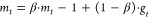

  14

  15
  (c) Adagrad: The second-order momentum is used, and the step size can be adjusted adaptively, but its second-order momentum accumulates the entire history, and the learning may be stopped early.

  16
  (d) AdaDelta/RMSProp: Second-order momentum is used, but its update method is different from AdaGrad. AdaGrad accumulates all historical second-order momentum, and AdaDelta accumulates part of it. It can avoid ending the study early.

  17
  (e) Adam: Adam combines the first-order momentum with the second-order momentum, which greatly accelerates the convergence rate. Its first-order momentum update method is the same as SGD with momentum; the second-order momentum update method is the same as AdaGrad.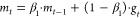

  18

  19

  (f) Adamax: Adamax is a variant of Adam. This method provides a simpler range formula change on the upper limit of the learning rate.

20

• (3)Calculate the descending gradient η_t at the current moment:

21

• (4)Update ω according to the descending gradient:

22

The difference between the different optimization algorithms is reflected in the different calculation methods of g_t, m_t, and V_t in steps (1) and (2).

3.2. Adamax Optimization Algorithm

The Adamax algorithm is a variant of Adam, and it sets a simpler range for the upper limit of the learning rate.

In Adamax, the gradient of formula 11 is calculated using formula 23

23

The first-order momentum is calculated using formula 24

24

The second-order momentum is calculated using formula 25

25

Among these variables, β₁ and β₂ are hyperparameters that control the first-order momentum and second-order momentum, respectively. Its value is determined by optimization algorithm.

Formula 23 is substituted into formulas 24 and 25, and then formulas 24 and 25 are substituted into formulas 21 and 22 to update the parameter ω.

4. Experiment

4.1. Experimental Data

A total of 103,598 monitoring data points obtained from a comprehensive coal mining face from 16:25:00 on January 2, 2019, to 23:50:00 on December 31, 2019, at a sampling interval of 5 min were used as the experimental data. Because of the partial absence of the original data, 1142 data points were missing. The original data were preprocessed by applying the Laida criterion and Lagrange interpolation method, and the number of processed data points was 104,740. The average value of the preprocessed data was 0.143033; the standard deviation was 0.083732; the minimum value was 0; and the maximum value was 0.984. The data were divided into a training set and a test set according to the ratio 9:1, and there were no missing or imputed data in the test set.

4.2. Evaluation Index

To test the effectiveness of the gas concentration forecasting method based on Adamax-BiGRU, a certain index must be used to comprehensively measure and evaluate the forecasting effect. Here, the MSE is used to evaluate the model.

Models using an RNN and LSTM are compared, as well as optimization algorithms using SGD, SGDM, NAG, RMSProp, AdaGrad, AdaDelta, and Adam.

4.3. Experimental Steps

The experiment is performed with the following steps:

Step 1: Data preprocessing. First, the Laida criterion is applied to address the noise in the gas concentration monitoring data.

Second, the Lagrange interpolation method is used to interpolate the missing values of the monitoring data to obtain the processed monitoring data.

Finally, the values of the application data set are normalized to [0, 1].

Step 2: The gas concentration time series monitoring data are spatially reconstructed, and input samples are constructed for training the Adamax-BiGRU model.

Step 3: The structure of the BiGRU neural network is determined—that is, the number of hidden layers of the BiGRU, the number of neurons in each layer, and the value of the epoch;

Step 4: In order to update and calculate the network parameters that affect the training and output of the BiGRU model, make it approximate or reach the optimal value, thereby minimizing the loss function. The Adamax optimization algorithm is applied to optimize the BiGRU model and establish a forecasting model;

Step 5: The model forecasting effect on the test set is verified, and the forecasting data is denormalized to visualize the forecasting result with MSE.

The MSE is the expected value of the square of the difference between the estimated value of the parameter ŷ_t and the true value of the parameter y_t. The calculation formula is as follows

26

Through the above five steps, gas concentration forecasting based on the Adamax-BiGRU model can be performed.

5. Results and Discussion

5.1. Determination of the Model Parameters

To determine the parameters of the Adamax-BiGRU model, the convergence of the MSE on the training set is compared for different parameter values to select the optimal number of hidden layers, the number of nodes in the hidden layers and the number of iterations. The following parameters are determined by comparison: the number of hidden layers is 2; the number of neurons is 32; the value of the batch size is 20; the learning rate is 0.01; and the number of iterations is 5.

First, the number of training rounds is preset to epochs = 100; then, the error of the BiGRU on the training set for each round is shown in Figure 5. It can be seen from Figure 5 that after epochs = 40, the training error and verification error are basically stable. Therefore, setting epochs = 40 can meet the training requirements.

Figure 5.

Error of the training set in the BiGRU with different epochs.

5.2. Comparison of Different Models

The same structure is constructed based on the RNN, LSTM, GRU, and BiGRU gas concentration forecasting models, and the optimization algorithm uses Adam. The experimental results of the RNN, LSTM, GRU, and BiGRU models on the test set are shown in Figures 6–9. All data are shown in subgraph (a), and the 6000th to the 6500th data are shown in Subgraph (b). The data comparison of the experimental results is shown in Table 1.

Figure 6.

Prediction effect of the RNN model on the test set. (a) All data of the test set. (b) 6000th to the 6500th data of the test set.

Figure 9.

Prediction effect of the BiGRU model on the test set. (a) All data of the test set. (b) 6000th to the 6500th data of the test set.

Table 1. Comparison of the Experimental Results of Different Models.

model	running time/s	MSE of the training set	MSE of the test set
RNN	4	0.000564	0.000563
LSTM	5	0.000517	0.000479
GRU	4	0.000477	0.000432
BiGRU	4	0.000457	0.000419

Figure 7.

Prediction effect of the LSTM model on the test set. (a) All data of the test set. (b) 6000th to the 6500th data of the test set.

Figure 8.

Prediction effect of the GRU model on the test set. (a) All data of the test set. (b) 6000th to the 6500th data of the test set.

From Figures 6–9, it can be seen that the forecasting effect of the RNN is poor, followed by LSTM, and the forecasting effect of the GRU and BiGRU models is good.

As seen from Table 1, the running time of the BiGRU is the same as that of the RNN, but the error of the training and test sets is reduced by 18.97 and 25.58%, respectively; compared to LSTM, the running time of the BiGRU is reduced by 25%, and the error of the training set and test set is reduced by 11.61 and 12.53%, respectively. Compared with the unidirectional GRU model, the running time is consistent, but the error of the training set and test set is reduced by 4.19 and 3.01%, respectively. Taken together, the BiGRU achieves the best forecasting results.

5.3. Comparison of the Different Optimization Algorithms

To further improve the forecasting effect of the BiGRU model, the GRU model is optimized. The experimental results of different optimization algorithms based on the GRU model are shown in Table 2, and the experimental results of different optimization algorithms based on the BiGRU model are shown in Table 3.

Table 2. Comparison of the Experimental Results of Different Optimization Algorithms for the GRU Model.

model	running time/s	MSE of the training set	MSE of the test set
SGD	3	0.000899	0.000836
SGDM	3	0.000470	0.000435
NAG	4	0.000469	0.000433
RMSProp	3	0.000459	0.000421
AdaGrad	4	0.000478	0.000439
AdaDelta	4	0.000474	0.000436
Adam	4	0.000463	0.000432
Adamax	4	0.000458	0.000423

Table 3. Comparison of the Experimental Results of Different Optimization Algorithms for the BiGRU Model.

model	running time/s	MSE of the training set	MSE of the test set
SGD	3	0.000544	0.000497
SGDM	3	0.000467	0.000433
NAG	5	0.000460	0.000428
RMSProp	3	0.000455	0.000415
AdaGrad	4	0.000471	0.000432
AdaDelta	4	0.000477	0.000433
Adam	4	0.000457	0.000419
Adamax	4	0.000447	0.000413

As seen in Tables 2 and 3, compared with other optimization algorithms, Adamax achieves the best forecasting effect on both the training set and the test set. Compared with the Adamax-GRU model and the Adamax-BiGRU model, the Adamax-BiGRU model achieves better forecasting results.

6. Conclusions and the Future Work

(1) A gas concentration forecasting algorithm based on Adamax-BiGRU is proposed, which forecasts gas concentration time series. (2) By comparing optimization algorithms, such as SGD, SGDM, NAG, RMSProp, AdaGrad, AdaDelta, Adam, and Adamax, the optimization algorithm for the BiGRU model that is most suitable for mine gas concentration data forecasting is determined to be Adamax. (3) The application to an actual data set shows that compared with the RNN and LSTM models, the Adamax-BiGRU model achieves better forecasting results with a lower time complexity and has greater practical application value. (4) In future work, the internal network structure of the BiGRU model will be further studied and optimized to achieve faster convergence speed and prediction accuracy.

The authors declare no competing financial interest.

References

- Liu Y. J.; Yuan L.; Xue J. H.; Tian Z. C. Analysis on the occurrence law of gas disaster accidents in coal mine from 2007 to 2016. Min. Saf. Environ. Protect. 2018, 45, 124–128. [Google Scholar]
- Yuan L. Innovation and development of safety science and technology in coal industry of China. Saf. Coal Mines 2015, 46, 5–11. [Google Scholar]
- He J.; Liu L. B.; Tang Y. J. Gas content prediction based on linear double exponential smooth method. Coal Sci. Technol. 2014, 42, 48–50. [Google Scholar]
- Guo S. W.; Tao Y. F.; Li C. Dynamic forecasting of gas concentration based on time series. Ind. Mine Autom. 2018, 44, 20–25. [Google Scholar]
- Zhao M. C.; He A. M.; Qu S. J. Research on time series forecasting method of gas data on fully mechanized mining face. Ind. Mine Autom. 2019, 45, 80–85. [Google Scholar]
- Ren X. D. Application research of gas concentration forecasting and early earning model in Luning Mine. Coal Mine Mod. 2020, 2, 47–49. [Google Scholar]
- Wang P.; Wu Y. P.; Wang S. L.; Wu X. M. Study on Lagrange-ARIMA real-time forecasting model of mine gas concentration. Coal Sci. Technol. 2019, 47, 141–146. [Google Scholar]
- Yao Q. H.; Qiu B. H. Prediction algorithm of gas concentration in coal mine based on improved BP neural network. Coal Technol. 2017, 36, 182–184. [Google Scholar]
- Zhou X. L.; Zhang G.; Lyu C.; Huang H. A grey model for predicting the gas content in the deep coal seam and its application via the neural network of the difference radial basis function. J. Saf. Environ. 2017, 17, 2050–2055. [Google Scholar]
- Li H.; Jia J.; Yang X. Y.; Song C. R. Gas concentration forecasting model for fully mechanized coal mining face. Ind. Mine Autom. 2018, 44, 48–53. [Google Scholar]
- Wang K. J.; Wang J. Y. Forecasting of gas concentration based on SVM optimized by memetic algorithm. Coal 2020, 29, 4–6. [Google Scholar]
- Gong S. F.; Li Y. S. Forecasting of underground gas concentration state based on data fusion. J. Xi’an Univ. Sci. Technol. 2018, 38, 506–514. [Google Scholar]
- Jia P. T.; Deng J. Coal mine gas concentration Combination prediction model based on universal average operation. China Saf. Sci. J. 2012, 22, 41–46. [Google Scholar]
- Zhang Z. Z.; Qiao J. F.; Yu W. Forecasting coalmine gas concentration based on dynamic neural Network. Contr. Eng. China 2016, 23, 478–483. [Google Scholar]
- Wang G. F.; Wang H.; Ren H. W.; Zhao G. R.; Pang Y. H.; Du Y. B.; Zhang J. H.; Hou G. 2025 scenarios and development path of intelligent coal mine. J. China Coal Soc. 2018, 43, 295–305. 10.13225/j.cnki.jccs.2018.0152. [DOI] [Google Scholar]
- Krizhevsky A.; Sutskever I.; Hinton G. E. ImageNet Classification with Deep Convolutional Neural Networks. Adv. Neural Inf. Process. Syst. 2012, 25, 1097–1105. [Google Scholar]
- Sak H.; Senior A. W.; Beaufays F. Long short term memory based recurrent neural network architectures for large vocabulary speech recognition. Comput. Sci. 2014, 13, 338–342. [Google Scholar]
- Sundermeyer M.; Schlüter R.; Ney H. LSTM neural networks for Language modeling. Interspeech 2012, 31, 601–608. [Google Scholar]
- Nammous M. K.; Saeed K.; Kobojek P. Using a small amount of text-independent speech data for a BiLSTM large-scale speaker identification approach. J. King Saud Univ. Comput. Inf. Sci. 2020, 10.1016/j.jksuci.2020.03.011. [DOI] [Google Scholar]
- Sánchez-Gutiérrez M. E.; González-Pérez P. P. Discriminative neural network pruning in a multiclass environment: A case study in spoken emotion recognition. Speech Commun. 2020, 120, 20–30. 10.1016/j.specom.2020.03.006. [DOI] [Google Scholar]
- Liu C.; Wang C.; Sun F. C.; Rui Y.. Image2 Text: a multimodal caption generator. ACM Multimedia, 2016; pp 746–748.
- Li W. S.; Wang L.; Wei C. Application and design of LSTM in coal mine gas forecasting and warning system. J. Xi’an Univ. Sci. Technol. 2018, 38, 1027–1035. [Google Scholar]
- Sun Z. Y.; Cao Y. L.; Yang D.; Han C. J.; Ma X. M.; Zhao Y. R. Dynamic forecasting of gas concentration in mining face based on long short-term memory neural network. Saf. Coal Mines 2019, 50, 152–157. [Google Scholar]
- Li S. G.; Ma L.; Pan S. B.; Shi X. L. Research on forecasting model of gas concentration based on RNN in coal mining face. Coal Sci. Technol. 2020, 48, 33–38. [Google Scholar]
- Ma L.; Pan S. B.; Dai X. G.; Song S.; Shi X. L. Gas concentration forecasting model of working face based on PSO-Adam-GRU. J. Xi’an Univ. Sci. Technol. 2020, 40, 363–368. [Google Scholar]
- Jia P.; Liu H.; Wang S.; Wang P. Research on a mine gas concentration forecasting model based on a GRU network. IEEE Access 2020, 8, 38023–38031. 10.1109/access.2020.2975257. [DOI] [Google Scholar]
- Yang Z.; Tian L.; Li C.. A Fast Video Shot Boundary Detection Employing OTSU’s Method and Dual Pauta Criterion. 2017 IEEE International Symposium on Multimedia (ISM), Taichung, 2017; pp 583–586. [Google Scholar]
- Li X.; Zhao J.; Zhao X.; Xu J.. Application of an Improved Lagrangian Interpolation Prediction Method in Continuous Power Flow Calculation. 2019 6th International Conference on Systems and Informatics (ICSAI), Shanghai, China, 2019; pp 209–212. [Google Scholar]
- Hochreiter S.; Schmidhuber J.; Schmidhuber J. Long short-term memory. Neural Comput. 1997, 9, 1735–1780. 10.1162/neco.1997.9.8.1735. [DOI] [PubMed] [Google Scholar]
- Cho K.; Van Merrienboer B.; Gulcehre C.; Bahdanau D.; Bougares F.; Schwenk H.; Bengio Y.. Learning phrase representations using RNN encoder-decoder for statistical machine translation. 2014, arXiv:1406.1078 [cs.CL]. [Google Scholar]