Spatial variations in the estimated production of reactive oxygen species in the epithelial lung lining fluid by iron and copper in fine particulate air pollution

Supplemental Digital Content is available in the text.

Abstract

Background:

Certain metals may play an important role in the adverse health effects of fine particulate air pollution (PM_2.5), but few models are available to predict spatial variations in these pollutants.

Methods:

We conducted large-scale air monitoring campaigns during summer 2016 and winter 2017 in Toronto, Canada, to characterize spatial variations in iron (Fe) and copper (Cu) concentrations in PM_2.5. Information on Fe and Cu concentrations at each site was paired with a kinetic multilayer model of surface and bulk chemistry in the lung epithelial lining fluid to estimate the possible impact of these metals on the production of reactive oxygen species (ROS) in exposed populations. Land use data around each monitoring site were used to develop predictive models for Fe, Cu, and their estimated combined impact on ROS generation.

Results:

Spatial variations in Fe, Cu, and ROS greatly exceeded that of PM_2.5 mass concentrations. In addition, Fe, Cu, and estimated ROS concentrations were 15, 18, and 9 times higher during summer compared with winter with little difference observed for PM_2.5. In leave-one-out cross-validation procedures, final multivariable models explained the majority of spatial variations in annual mean Fe (R² = 0.68), Cu (R² =0.79), and ROS (R² = 0.65).

Conclusions:

The combined use of PM_2.5 metals data with a kinetic multilayer model of surface and bulk chemistry in the human lung epithelial lining fluid may offer a novel means of estimating PM_2.5 health impacts beyond simple mass concentrations.

What this study adds

Certain metal components in PM_2.5 are thought to contribute to air pollution health effects. However, few models are available to estimate exposures for individual metals or their impact on important biological mechanisms such as oxidative stress. In this study, we combined data for PM_2.5 iron and copper with a kinetic multilayer model of surface and bulk chemistry in the lung epithelial lining fluid. In doing so, we estimated the impact that these metals may have on the production of reactive oxygen species in exposed populations. The models presented offer a novel means of estimating PM_2.5 health impacts in population-based studies.

Ambient fine particulate air pollution (PM_2.5) is associated with a range of adverse cardiovascular and respiratory outcomes and is an important contributor to global disease burden.¹ However, surprisingly little is known about the specific components/sources of PM_2.5 that are most relevant to health and exposures are traditionally assigned as particle mass concentrations.

Of the potential candidates, metal components in PM_2.5 are thought to play an important role in determining overall PM_2.5 health effects owing to their ability to cause oxidative stress in biological systems.^2,3 However, few models are available to estimate spatial variations in PM_2.5 metal concentrations for use in population-based studies.⁴ Moreover, separating the individual health effects of specific metal components remains a challenge owing to strong correlations between elements.⁴ An alternative approach is to examine the combined impact of multiple elements based on a shared mechanisms of action: oxidative stress.

Lakey et al⁵ recently developed a kinetic multilayer model of surface and bulk chemistry in the lung epithelial lining fluid (KM-SUB-ELF). This model can be used to estimate reactive oxygen species (ROS) concentrations (nM; i.e., OH, HO₂, O₂⁻, H₂O₂) generated in the human respiratory tract in response to inhaled pollutants including Cu and Fe in PM_2.5. Briefly, the KM-SUB-ELF model estimates ROS generation in the lung epithelial lining fluid by resolving mass transport and chemical reactions between pollutants and antioxidants/surfactants in the lung.⁵ This model provides chemical baseline estimates of exogenous ROS concentrations generated in response to Fe and Cu in PM_2.5 but does not resolve endogenous ROS generated via biological interactions and/or responses of the immune system. Nevertheless, this model may provide a useful means of estimating the combined health impacts of Fe and Cu in PM_2.5.

In this study, our goal was to characterize possible spatial variations in the combined impact of Fe and Cu in PM_2.5 on ROS production in exposed populations by combining spatial monitoring data with the KM-SUM-ELF model. Land use regression models were developed to predict spatial variations in ROS, Fe, and Cu in Toronto, Canada, for use in future cohort studies.

Methods

Spatial monitoring study

Two large-scale PM_2.5 monitoring campaigns were conducted across Toronto, Canada, during August/September 2016 (summer) and February/March 2017 (winter). During summer sampling, daily mean temperatures ranged from 18.3°C to 27.2°C, whereas winter temperatures ranged from −8.8°C to 7.5°C. Total precipitation was similar during summer (38.2 mm) and winter (39.7 mm) sampling periods.

Monitoring sites were identified to capture the variability of microenvironments in Toronto while maximizing spatial coverage. A neighborhood map of the city was used whereby each neighborhood was characterized in terms of road density, population density, employment density, and percentage of commercial land use. Neighborhoods were then grouped into a predetermined number of clusters (30 clusters) using a k-means clustering technique such that internal similarities were maximized, whereas similarities between groups were minimized. Finally, sites were identified manually, maximizing spatial coverage, while ensuring that two to three sites were in each cluster. In total, 67 sites were successfully monitored in summer and 42 sites were monitored in winter with 28 sites monitored during both seasons (a map of the monitoring locations is shown in Supplemental Figure S1; http://links.lww.com/EE/A16).

Integrated 2-week samples were collected at each site using Teflon filters with cascade impactors at a flow rate of 5 L/min. During each campaign, all PM_2.5 samples were collected simultaneously using preset pump timers and separate sampling kits at each location. This eliminated the need to adjust for temporal differences in air pollution concentrations between sites as all sites were monitored over exactly the same time period. PM_2.5 mass concentrations were determined gravimetrically before metals analysis by x-ray fluorescence (XRF).

PM_2.5 metals analyses

Copper and iron concentrations in PM_2.5 samples were determined using x-ray fluorescence (XRF) according to United States Environmental Protection Agency (EPA) Method IO-3.3 in Compendium of Methods for the Determination of Metals in Ambient Particulate Matter (EPA 625/R-96/010a). Concentrations of 31 other elements were also obtained and were used primarily for correlations analyses and to identify common groupings of elements. Throughout this paper, Fe and Cu refer to concentrations in PM_2.5.

Estimating reactive oxygen species concentrations using a kinetic multilayer model of surface and bulk chemistry in the lung epithelial lining fluid model

The KM-SUB-ELF model was recently developed and described in detail by Lakey et al.⁵ Briefly, the model consists of a surface surfactant layer containing lipids and proteins and the epithelial lining fluid bulk with a thickness of 0.5 μm, which is the average thickness of ELF in bronchi.⁶ The bulk layer contains four antioxidants: ascorbate, uric acid, glutathione, and α-tocopherol at concentrations of 40, 207, 109, and 0.7 μM, respectively, which are typical concentrations in the bronchoalveolar region of the respiratory tract.^6,7 Mass transport and over 50 chemical reactions are explicitly treated in the model. The reactions are listed alongside their rate coefficients in the supplementary information of Lakey et al⁵ and include the reactions of ROS with antioxidants and surfactants, the formation of ROS from the redox cycling of Fe and Cu ions with ascorbate and oxygen, the interconversion of ROS due to Fenton and Fenton-like chemistry, and the destruction of O₂⁻ radicals due to the presence of the superoxide dismutase enzyme.^8,9 The concentration of Fe and Cu ions in the epithelial lining fluid was estimated using known airborne concentrations of Fe and Cu in PM_2.5 according to the following equation:

where MW is the molecular weight of the species, breathing rate was assumed to be 1.5 m³/h,^10,11 PM deposition rate was set to 45%,¹² and total ELF volume was 20 ml.^13,14 The fractional solubilities of Fe and Cu were assumed to be 0.1 and 0.4, respectively.^15–17 Error bars for the different ROS concentrations were calculated by varying the range of Fe and Cu fractional solubilities between 0.05 and 0.25 and 0.2 and 0.6, respectively.⁵ These ranges of solubilities for Fe and Cu were considered to recognize the fact that XRF analyses do not reveal the precise structure of metal speciation complexes which can impact solubility in the lung lining fluid. The accumulation time was set to 2 hours as inhaled particles can accumulate in the respiratory tract over several hours before they are removed by the immune system and metabolic activity.¹⁸ It is important to note that ROS concentrations obtained from KM-SUB-ELF model simulations estimate exogenous ROS concentrations generated in the lung in response to Fe and Cu; endogenous ROS generated through biological interactions (e.g., ROS generation from macrophage activation) are not considered in the calculations.

Extraction of land use and traffic parameters for land use regression models

Various land use and built environment attributes were derived for each monitoring site using ArcMap 10.4.1 (ESRI, Redlands, CA). Land use composition was computed within circular buffers of 100, 200, 300, 500, 700, and 1000 meters and included specific categories for residential, commercial, governmental/institutional, resource/industrial, parks, open area, water, and building footprints (DMTI Spatial (Database 2014), Richmond Hill, Ontario, Canada). Moreover, the length of bus routes, highways, major roads, and rail lines were derived in each buffer (City of Toronto Open Data portal 2016). Other variables computed within the buffers included population density (Toronto Neighbourhood and Demographics data of 2013), mean and maximum building height, number of bus stops, number of road intersections, and number of trees (City of Toronto Open Data portal 2016). Finally, the average hourly traffic volume between 6 am and 7 pm was derived using a traffic assignment model and an Origin-Destination (OD) matrix of trips extracted from the Transportation Tomorrow Survey (TTS) (year 2011) for the Greater Toronto and Hamilton Area (GTHA). Distances between each sampling location and the closest rail line, major road, highway, Pearson airport, shore, City Center, and industrial NOx and PM emitting facility (National Pollutant Release Inventory website of the Government of Canada) were also estimated and squared terms were also examined for these parameters during model development.

Statistical analyses

Multivariable linear regression models were used to estimate spatial variations in Fe, Cu, and their impact on ROS generation in the human respiratory tract. Separate models were developed for summer (based on 67 sites) and for annual mean concentrations as too few sites were available to justify separate models for winter. The database for annual mean concentrations was generated by averaging values across the summer and winter seasons. For sites missing winter PM_2.5 data, multivariable linear regression models were used to predict missing values (i.e., for winter PM_2.5, Fe, and Cu) based on PM_2.5 mass and composition data from the 28 sites with complete data for both seasons. These predictive models are shown in Supplemental Table S1; http://links.lww.com/EE/A16 and had R² values ranging from 0.70 to 0.82. R² values decreased in leave-one-out cross-validation procedures (ranging from 0.55 for Fe to 0.37 for PM_2.5), but root mean square errors remained low (e.g., 0.79 μg/m³ for PM_2.5) (Supplemental Table S1; http://links.lww.com/EE/A16). In total, models for annual averages are based on data for 67 sites.

Fe and Cu concentrations were modeled as percentages of total PM_2.5 mass concentrations (e.g., Fe/PM_2.5 × 100%) to improve model fit (relative to absolute metal concentrations) and to reduce correlations between the two elements. Models for ln(Fe) and ln(Cu) are presented in the supplemental material (Tables S4 and S5; http://links.lww.com/EE/A16) but are not discussed further as they did not perform as well as models for proportions of Fe and Cu in PM_2.5. Our model building procedure followed several steps: (1) Single variable linear regression models were examined for each of the candidate predictor variables outline above; (2) Variables that were associated with the outcome (i.e., 95% confidence interval excluded the null) were retained for potential inclusion in the final model; (3) Spearman’s correlations were determined for the candidate predictors identified in step 2 and highly correlated variables (r > 0.7) were removed (retaining the best predictor of each correlated pair); for parameters with multiple buffer sizes, the buffer size that was most strongly associated with the outcome was retained; and (4) All parameters retained after step 3 were included in the model; “nonsignificant” parameters were only removed if doing so improved model fit (i.e., increased the adjusted R² value and decreased the root mean square error). We did not impose preconceived rules on the direction of effects for parameters included in the model. A leave-one-out cross-validation procedure was used to evaluate final model performance using the loocv procedure in Stata version 15 (Statacorp, College Station, Texas).

Correlations between individual PM_2.5 metal components were examined to evaluate potential sources of these contaminants. Specifically, we visualized these relationships using the qgraph and corrplot packages in R (version 3.3.0). The “spring” layout in the qgraph package displays correlations between metals as a network: more highly correlated nodes are grouped together and are linked by thinker, more darkly colored lines.

Mapping the land use regression models

Maps of exposure surfaces were generated by first dividing the city of Toronto into grid cells of 100 × 100 meters using ArcMap. Next, the final set of predictors for land use regression models for Fe, Cu, and ROS were computed for the mid-point of each grid cell. Finally, the predicted values for each mid-point were calculated and associated with the corresponding grid cell for mapping.

Results

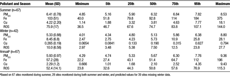
Descriptive statistics for ambient PM_2.5 mass concentrations and Fe, Cu, and their estimated impact on ROS generation in the lung lining fluid are shown in Table. In general, spatial variations in Fe, Cu, and ROS greatly exceeded that of PM_2.5 mass concentrations. In addition, Fe, Cu, and ROS concentrations were 15, 18, and 9 times higher during summer compared with winter, respectively, with little difference observed for PM_2.5 mass concentrations (Supplemental Figure S2; http://links.lww.com/EE/A16). As expected, correlations between metals in PM_2.5 were high (Figure 1 and Supplemental Figure S3; http://links.lww.com/EE/A16) and suggested three primary groupings: (1) One containing elements such as Fe, Cu, and Ba that are associated with roadway emissions including brake ware^19,20; (2) One containing crustal elements (i.e., Al, Si, Ca) related to resuspended soil; and (3) A grouping of Mn and Zn. As ROS concentrations were derived from Fe and Cu, Spearman correlations between summer Fe and Cu and ROS were high at 0.93 and 0.95, respectively. Correlations between annual ROS concentrations and Fe and Cu were 0.94 and 0.96, respectively.

Figure 1.

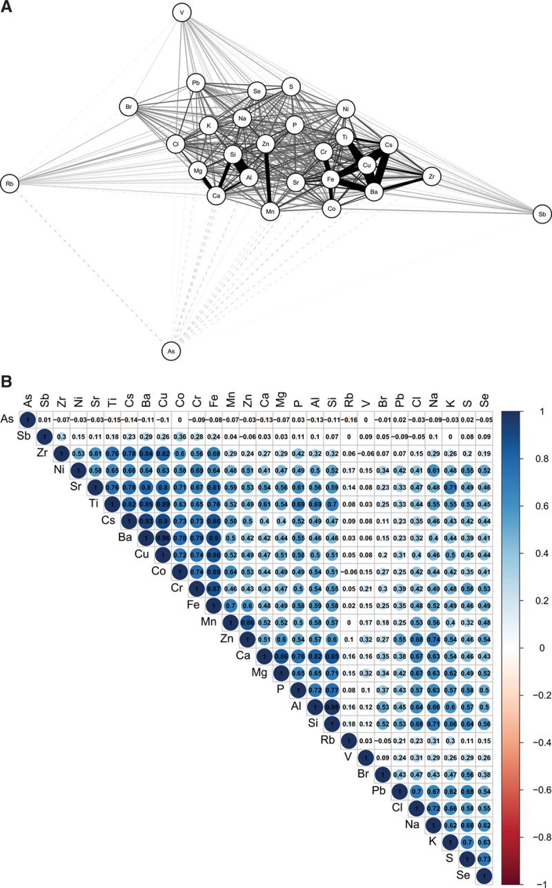
Correlations between PM_2.5 metals during summer. A, Network plot with more highly correlated metals grouped more closely together and linked by darker, thicker lines (dashed lines indicate inverse correlations). Numeric correlation values are illustrated in B.

Table.

Descriptive Statistics for PM2.5 (μg/m3), Fe (ng/m3), Cu (ng/m3), and the Estimated Impact of Fe and Cu on ROS (nM) in Toronto, Canada

Final land use regression models for Fe, Cu, and their estimated impact on ROS generation in the human lung are shown in Figure 2 (summer) and Figure 3 (annual). Standardized model coefficients (and 95% confidence intervals) and cross-validation results are also presented in Supplemental Tables S2 and S3; http://links.lww.com/EE/A16. In general, models for Cu performed best with cross-validation R² values of 0.77 and 0.79 for the summer and annual models, respectively. Spatial variations in Cu were predominantly explained by variables related to traffic proximity, although population density was also included in the annual model. Traffic parameters were also important determinants of Fe, but other factors including rail line proximity (or length of rail lines within a 1000 meters buffer) and proximity to Pearson airport were also identified as important determinants of Fe concentrations; cross-validation R² values for the summer and annual mean Fe models were 0.53 and 0.68, respectively.

Figure 2.

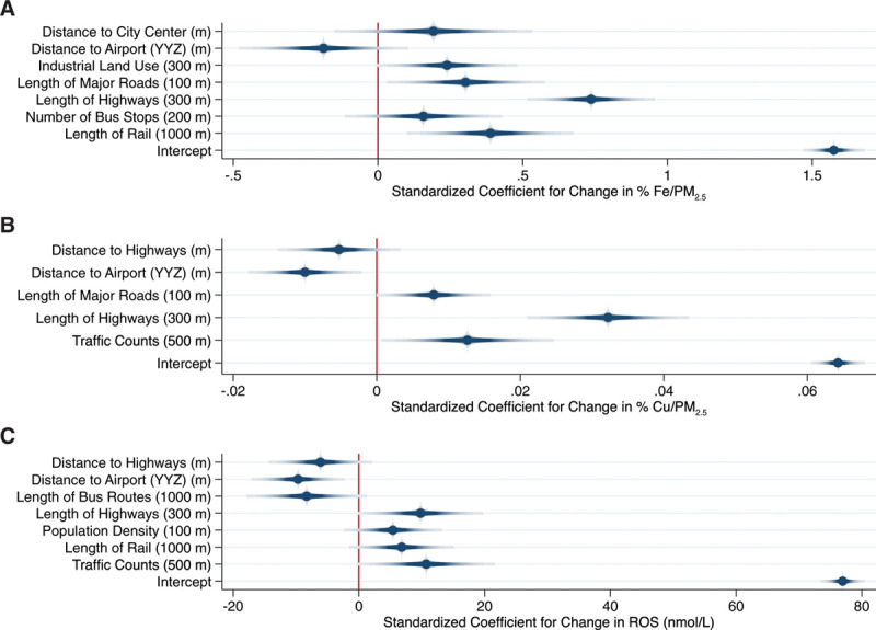
Land use regression models for Fe (% mass), (A: Model R² = 0.68; Cross-validation R² = 0.53), Cu (% mass), (B: Model R² = 0.81; Cross-validation R² = 0.77), and their estimated impact on ROS (C: Model R² = 0.64; Cross-validation R² = 0.56) during summer in Toronto, Canada. Dots and shaded lines reflect point estimates and 95% confidence intervals.

Figure 3.

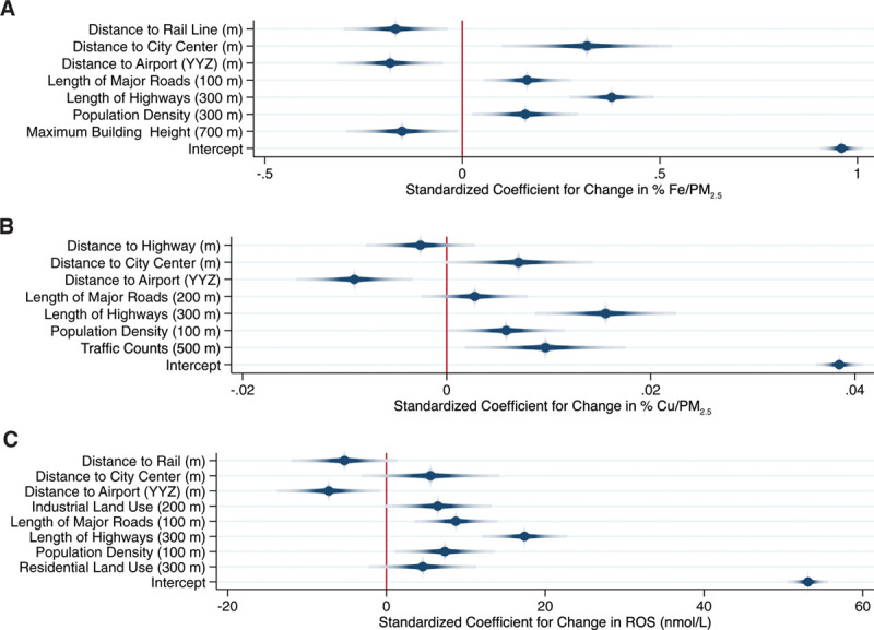
Land use regression models for annual mean Fe (% mass) (A: Model R² = 0.72; Cross-validation R² = 0.68), Cu (% mass) (B: Model R² = 0.81; Cross-validation R² = 0.79), and their estimated impact on ROS (C: Model R² = 0.71; Cross-validation R² = 0.65) in Toronto, Canada. Dots and shaded lines reflect point estimates and 95% confidence intervals.

Not surprisingly, final ROS models reflected components of both the Fe and Cu models with length of highways within 300 meters being the strongest predictor of ROS in both summer and annual models. Other important predictors of annual mean ROS generation included rail line proximity, population density, proximity to Pearson airport, and industrial land use within 200 meters. Distance to city center appeared in all three annual models with increasing distance from city center associated with higher concentrations. This primarily reflects the fact that Toronto is surrounded by major highways/roadways, and thus, moving further from the city center brings you closer to these major sources of exposure. Mean variance inflation factors were less than 2 for all final models.

Exposure surfaces for summer and annual mean Fe, Cu, and their estimated combined impact on ROS are shown in Figure 4. These surfaces highlight the elevated concentrations of PM_2.5 metals during the summer months and their subsequent increased capacity to generate ROS in the lung during this time period. In particular, two areas of the Fe and ROS surfaces stand out in the upper right and lower left-hand corners of each surface: these areas reflect large rail yards which appear to be important local sources of iron in PM_2.5. Scatter plots are available in Supplemental Figures S4 and S5; http://links.lww.com/EE/A16 illustrating the relationship between PM_2.5, Fe, Cu, and total ROS concentrations as well as specific ROS species (which are dominated by H₂O₂). Interestingly, the scatter plot in Figure 5 illustrates that equivalent PM_2.5 mass concentrations can contribute to the generation of substantially different ROS concentrations (often differing by more than a factor of 2) owing to large seasonal differences in Fe and Cu.

Figure 4.

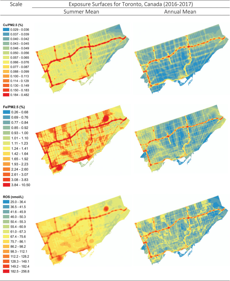
Land use regression surfaces for summer and annual mean Fe (% mass), Cu (% mass), and their estimated combined impact on ROS generation (nM).

Figure 5.

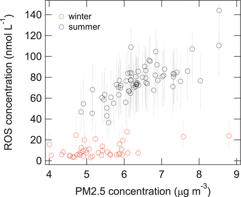
Estimated concentrations of ROS generated in lung epithelial lining fluid by PM_2.5 during summer and winter in Toronto, Canada, using the KM-SUB-ELF model. Error bars reflect uncertainty related to assumed solubilities for Fe and Cu.

Discussion

Surprisingly little is known about the specific components of PM_2.5 that are most relevant to health and population-based exposure assessment continues to rely on bulk particle mass concentrations. Metal components in PM_2.5 are generally thought to play an important role in determining overall PM_2.5 health effects^2,3; however, few models are available to predict exposures in epidemiological studies and separating the individual effects of specific metals remains a challenge.

In this study, we combined information on Fe and Cu in PM_2.5 with a kinetic multilayer model of surface and bulk chemistry in the epithelial lining fluid to estimate the impact of these metals on the production of ROS in the human lung lining fluid. In general, our findings suggest that spatial variations in Fe, Cu, and their combined impact on ROS are considerably greater than spatial variations in PM_2.5 mass concentrations. Moreover, our results suggest that large seasonal differences may exist in PM_2.5 metal concentrations that ultimately lead to more ROS production in response to PM_2.5 during the summer months. This seasonal difference is likely explained by increased snow cover/rain during the winter months in Toronto which would tend to minimize particle resuspension. More importantly, this finding suggests that resuspended particles containing metals from sources such as brake wear^19,20 (or rail lines) may be an interesting target for future risk management activities (in addition to direct tailpipe emissions) if ROS is ultimately tied to adverse health effects. Furthermore, our results indicate that equivalent PM_2.5 mass concentrations may elicit dramatically different biological responses; therefore, if the generation of ROS is an important mechanism contributing to PM_2.5 health effects, relying solely on PM_2.5 mass concentrations likely contributes substantially to exposure measurement error in epidemiological studies even if the mass concentrations themselves are measured without error.

Our findings also shed light on an important ongoing question in air pollution epidemiology: Why do we continue to see important health effects at very low PM_2.5 mass concentrations? Whereas PM_2.5 mass concentrations in Toronto were low and the range was small (≈4–9 μg/m³), spatial variations in the estimated impact of Fe and Cu on ROS generation were much larger; therefore, a 1-unit change in exposure on the scale of PM_2.5 mass concentration likely translates into a much larger change on the ROS scale which ultimately may be more biologically relevant. Moreover, it is important to note that the predicted magnitude of ROS generation in response to Fe and Cu (i.e., more than 200 nM in some areas during summer) is biologically relevant as normal human ROS concentrations are approximately 100 nM and elevated H₂O₂ concentrations have been observed in respiratory disease patients including adult asthmatics. ^5,21–23 Moreover, although the ROS model contained many of the same predictors as the Fe and Cu models, the added value of the ROS models relates to the fact that it estimates the combined impact of these two components on ROS using a single parameter rather than two separate parameters. Indeed, separating the individual health impacts of Cu and Fe is difficult owing to colinearity and the use of a single parameter to estimate their combined impact on an important mechanism of action seems advantageous. However, all three models should be explored in future epidemiological studies to verify this hypothesis.

To our knowledge, this is the first study to model spatial variations in the combined impact of Fe and Cu in PM_2.5 on ROS generation in the human lung. Indeed, such models are of interest as the application of oxidative stress assays (primarily related to the depletion of dithiothreitol or antioxidants such as glutathione) has gained significant traction in the epidemiological literature as several studies have reported stronger associations with these new metrics than with traditional PM_2.5 mass concentrations.^24–26 Nevertheless, recent evidence also suggests that it is important to consider both ROS generation and antioxidant depletion as common oxidative potential assays including the dithiothreitol (DTT) assay may not capture the ROS activity of some PM components including Fe.²⁷ Moreover, it is not clear how ROS generation estimated using the KM-SUB-ELF model may relate to other common particle oxidative potential assays including DTT, electron spin resonance (ESR), or ascorbate/glutathione depletion. To date, existing evidence suggests that ROS generation estimated using Fe and Cu concentrations in the KM-SUB-ELF model is at least moderately correlated with these metrics.^28–31 For example, a recent evaluation of five oxidative potential metrics for PM₁₀ samples reported correlations for Cu and the above oxidative potential assays ranging from 0.48 to 0.87 with a similar range of correlations observed for Fe (0.48–0.71).³¹ Ultimately, the more important question is which of these assays is the best predictor of adverse health effects and which (if any) are superior to particle mass concentration in this respect. At a minimum, the KM-SUB-ELF model may serve as a cost-effective means of estimating the oxidative potential of airborne particles when Fe and Cu data are available in the absence of filter media (e.g., historical data) or when detailed chemical analyses of filter samples are not possible.

Although this study had many important advantages including a large simultaneous monitoring network for PM_2.5 metals and numerous geographic predictor variables, it is important to note several limitations. First, only 28 sites had monitoring data for both summer and winter; therefore, winter data had to be predicted for many sites used in the annual models. However, models used to predict missing data performed well with high R² values and low root mean square errors (RMSE). One exception was the model for winter PM_2.5 which had a lower R² value in leave-one-out cross-validation procedures but also a low RMSE. Ultimately, prediction error in the outcome variables used in annual models likely contributed to greater uncertainty (i.e., wider 95% confidence intervals) in the slopes for independent variables in land use regression models but would not bias the slopes for these variables.

It is also important to note that estimated values for ROS reflect exogenous ROS concentrations generated in the lung in response to Fe and Cu in PM_2.5 and not total ROS generated in response to the entire pollutant mixture. Indeed, additional ROS may be produced through biological responses not considered by the model (e.g., macrophage activation) or in response to ambient O₃ or quinones which can be handled by KM-SUB-ELF but were not considered here owing to the absence of monitoring data. Therefore, model estimates of ROS presented here likely underestimate the total oxidative burden caused by inhaled pollutant mixtures. Future studies should aim to incorporate O₃ and quinone measurements to obtain a more complete picture of the overall impact of ambient air pollution mixtures on ROS generation in the human lung. Moreover, model estimates of ROS generation are not intended to capture individual-level differences in ROS production owing to variance in factors such as age, genetics, or disease status. Rather, the KM-SUB-ELF model provides estimates of ROS generation under a certain set of conditions (described in the Methods section), thus allowing us to evaluate potential spatial differences in ROS generation in conjunction with PM_2.5 metals. In particular, our results reflect a range of assumed metal solubilities in the epithelial lung lining fluid and it is possible that the ranges used in this study do not adequately capture seasonal variations in metal solubilities or differences in solubilities between sampling sites. Likewise, our model does not include other transition metals that could contribute to the generation of ROS in the lung. As noted above, the overall consequence of these limitations is likely an underestimation of the impact of PM_2.5 components on ROS generation as well as imprecise estimation of spatial differences in ROS generation if metal solubilities differed substantially between monitoring sites.

In summary, we developed a model to estimate spatial variations in the impact of PM_2.5 metals on the generation of ROS in the human lung lining fluid in Toronto, Canada. Estimated spatial variations in ROS generation exceeded that of PM_2.5 mass concentrations and seasonal differences suggested that summer PM_2.5 contributes more to ROS than winter likely owing to decreased particle resuspension during the winter months. Our findings highlight the potential importance of nontailpipe emission sources (e.g., brake/rail ware) with respect to PM_2.5 and the combined use of PM_2.5 metals data with a kinetic multilayer model of surface and bulk chemistry in the human lung epithelial lining fluid may offer a novel means of estimating PM_2.5 health impacts beyond simple mass concentrations.

Conflicts of interest statement

The authors declare that they have no conflicts of interest with regard to the content of this report.

This study was supported by Health Canada and a Collaborative Health Research Projects Grant (Canadian Institute for Health Research (CIHR)/Natural Sciences and Engineering Research Council of Canada (NSERC)). S.W. also received support from a GRePEC salary award funded by the Cancer Research Society, the Quebec Ministry of Economy, Science and Innovation, and FRQS (Fonds de Recherche du Québec-Santé).

Data Access: Data and code are available upon request.

Acknowledgments

We would like to thank Hongyu You, David Van Rijswijk, Keith Van Ryswyk, Angelos Anastassopoulos, and Arman Ganji for helping with data collection during the field campaigns.

Supplementary Material

ee9-2-e020-s001.pdf ^{(774.5KB, pdf)}

References

- 1.GBD 2015 Risk Factors Collaborators. Global, regional, and national comparative risk assessment of 79 behavioural, environmental and occupational, and metabolic risks or clusters of risks, 1990–2015: a systematic analysis for the Global Burden of Disease Study 2015. Lancet. 2016;388:1659–1724. doi: 10.1016/S0140-6736(16)31679-8. [DOI] [PMC free article] [PubMed] [Google Scholar]
- 2.Valko M, Rhodes CJ, Moncol J, Izakovic M, Mazur M. Free radicals, metals and antioxidants in oxidative stress-induced cancer. Chemico-Biol Inter. 2006;160:1–40. doi: 10.1016/j.cbi.2005.12.009. [DOI] [PubMed] [Google Scholar]
- 3.Li N, Hao M, Phalen RF, Hinds WC, Nel AE. Particulate air pollutants and asthma: a paradigm for the role of oxidative stress in PM-induced adverse health effects. Clin Immunol. 2003;109:250–265. doi: 10.1016/j.clim.2003.08.006. [DOI] [PubMed] [Google Scholar]
- 4.Zhang J, Sun L, Barrett O, Bertazzon S, Underwood FE, Johnson M. Development of land-use regression models associated with airborne particulate matter in a North American city. Atmos Environ. 2015;106:165–177. [Google Scholar]
- 5.Lakey PSJ, Berkemeier T, Tong H, Arangio AM, Lucas K, Poschl U, Shiraiwa M. Chemical exposure-response relationship between air pollutants and reactive oxygen species in the human respiratory tract. Sci Rep. 2016;6:32916. doi: 10.1038/srep32916. [DOI] [PMC free article] [PubMed] [Google Scholar]
- 6.Mudway IS, Kelly FJ. Ozone and the lung: a sensitive issue. Mol Aspects Med. 2000;21:1–48. doi: 10.1016/s0098-2997(00)00003-0. [DOI] [PubMed] [Google Scholar]
- 7.van der Vliet A, O’Neill CA, Cross CE, et al. Determination of low-molecular-mass antioxidant concentrations in human respiratory tract lining fluids. Am J Physiol Lung C. 1999;276:L289–L296. doi: 10.1152/ajplung.1999.276.2.L289. [DOI] [PubMed] [Google Scholar]
- 8.Winterbourn CC. Reconciling the chemistry and biology of reactive oxygen species. Nature Chem Biol. 2008;4:278–286. doi: 10.1038/nchembio.85. [DOI] [PubMed] [Google Scholar]
- 9.Pöschl U, Shiraiwa M. Multiphase chemistry at the atmosphere–biosphere interface influencing climate and public health in the anthropocene. Chem Rev. 2015;115:4440–4475. doi: 10.1021/cr500487s. [DOI] [PubMed] [Google Scholar]
- 10.Spier C, Little D, Trim S, Johnson T, Linn W, Hackney J. Activity patterns in elementary and high school students exposed to oxidant pollution. J Expo Anal Env Epid. 1991;2:277–293. [PubMed] [Google Scholar]
- 11.U.S. EPA. Washington, DC: U.S. Environmental Protection Agency; Exposure Factors Handbook 2011 Edition (Final Report). EPA/600/R-09/052F, 2011. [Google Scholar]
- 12.Sarangapani R, Wexler AS. The role of dispersion in particle deposition in human airways. Toxicol Sci. 2000;54:229–236. doi: 10.1093/toxsci/54.1.229. [DOI] [PubMed] [Google Scholar]
- 13.Rennard S, Basset G, Lecossier D, et al. Estimation of volume of epithelial lining fluid recovered by lavage using urea as marker of dilution. J Appl Physiol. 1986;60:532–538. doi: 10.1152/jappl.1986.60.2.532. [DOI] [PubMed] [Google Scholar]
- 14.Walters DV. Lung lining liquid–the hidden depths. Neonatology. 2002;81(1 suppl):2–5. doi: 10.1159/000056764. [DOI] [PubMed] [Google Scholar]
- 15.Connell DP, Winter SE, Conrad VB, Kim M, Crist KC. The Steubenville Comprehensive Air Monitoring Program (SCAMP): concentrations and solubilities of PM2.5 trace elements and their implications for source apportionment and health research. J Air Waste Manage. 2006;56:1750–1766. doi: 10.1080/10473289.2006.10464580. [DOI] [PubMed] [Google Scholar]
- 16.Manousakas M, Papaefthymiou H, Eleftheriadis K, Katsanou K. Determination of water-soluble and insoluble elements in PM2.5 by ICP-MS. Sci Total Environ. 2014;493:694–700. doi: 10.1016/j.scitotenv.2014.06.043. [DOI] [PubMed] [Google Scholar]
- 17.Heal MR, Hibbs LR, Agius RM, Beverland LJ. Total and water-soluble trace metal content of urban background PM10, PM2.5 and black smoke in Edinburgh, UK. Atmos Environ. 2005;39:1417–1430. [Google Scholar]
- 18.Ghio AJ, Turi JL, Yang F, Garrick LM, Garrick MD. Iron homeostasis in the lung. Biol Res. 2006;39:67–77. doi: 10.4067/s0716-97602006000100008. [DOI] [PubMed] [Google Scholar]
- 19.Grigoratos T, Martini G.Non-exhaust traffic related emissions. Brake and tyre wear PM. European Commission Joint Research Science Centre. Report EUR 26648 EN. Available at: http://publications.jrc.ec.europa.eu/repository/bitstream/JRC89231/jrc89231-online%20final%20version%202.pdf. Accessed May 6, 2018.
- 20.Schauer JJ, Lough GC, Shafer MM, et al. Characterization of metals emitted from motor vehicles. Res Rep Health Eff Inst. 2006;133:1–76. [PubMed] [Google Scholar]
- 21.Aldakheel FM, Thomas PS, Bourke JE, Matheson MC, Dharmage SC, Lowe AJ. Relationship between adult asthma and oxidative stress markers and pH in exhaled breath condensate: a systematic review. Allergy. 2016;71:741–757. doi: 10.1111/all.12865. [DOI] [PubMed] [Google Scholar]
- 22.Kietzmann D, Kahl R, Müller M, Burchardi H, Kettler D. Hydrogen peroxide in expired breath condensate of patients with acute respiratory failure and with ARDS. Intensive Care Med. 1993;19:78–81. doi: 10.1007/BF01708366. [DOI] [PubMed] [Google Scholar]
- 23.Corradi M, Pignatti P, Brunetti G, et al. Comparison between exhaled and bronchoalveolar lavage levels of hydrogen peroxide in patients with diffuse interstitial lung diseases. Acta Biomed. 2008;79(1 suppl):73–78. [PubMed] [Google Scholar]
- 24.Weichenthal S, Lavigne E, Evans G, Pollitt K, Burnett RT. Ambient PM2.5 and risk of emergency room visits for myocardial infarction: impact of regional PM2.5 oxidative potential: a case-crossover study. Environ Health. 2016;15:46. doi: 10.1186/s12940-016-0129-9. [DOI] [PMC free article] [PubMed] [Google Scholar]
- 25.Strak M, Janssen N, Beelen R, et al. Long-term exposure to particulate matter, NO2, and oxidative potential of particualtes and diabetes in a large national health survey. Environ Int. 2017;108:228–236. doi: 10.1016/j.envint.2017.08.017. [DOI] [PubMed] [Google Scholar]
- 26.Maikawa CL, Weichenthal S, Wheeler A, et al. Particulate oxidative burden as a predictor of exhaled nitric oxide in children with asthma. Environ Health Perspect. 2016;124:1616–1622. doi: 10.1289/EHP175. [DOI] [PMC free article] [PubMed] [Google Scholar]
- 27.Xiong Q, Yu H, Wang R, Wei J, Verma V. Rethinking the dithiothreitol (DTT) based PM oxidative potential: measuring DTT consumption versus ROS generation. Environ Sci Technol. 2017;51:6507–6514. doi: 10.1021/acs.est.7b01272. [DOI] [PubMed] [Google Scholar]
- 28.Janssen NAH, Yang A, Strak M, et al. Oxidative potential of particulate matter collected at sites with different source characteristics. Sci Total Environ. 2014;472:572–581. doi: 10.1016/j.scitotenv.2013.11.099. [DOI] [PubMed] [Google Scholar]
- 29.Hellack B, Quass U, Nickel C, Wick G, Schins RPF, Kuhlbusch AJ. Oxidative potential of particulate matter at a German motorway. Environ Sci Processes Impacts. 2015;17:868–876. doi: 10.1039/c4em00605d. [DOI] [PubMed] [Google Scholar]
- 30.Boogaard H, Janssen NAH, Fischer PH, et al. Contrasts in oxidative potential and other particulate matter characteristics collected near major streets and background locations. Environ Health Perspect. 2012;120:185–191. doi: 10.1289/ehp.1103667. [DOI] [PMC free article] [PubMed] [Google Scholar]
- 31.Calas A, Uzu G, Kelly FJ, et al. Comparison between five acellular oxidative potential measurement assays performed with detailed chemistry on PM10 samples from the city of Chamonix (France). Atmos Chem Phys. 2017;18:7863–7875. [Google Scholar]