Efficient Estimation of Formation Enthalpies for Closed-Shell Organic Compounds with Local Coupled-Cluster Methods

Abstract

Efficient estimation of the enthalpies of formation for closed-shell organic compounds via atom-equivalent-type computational schemes and with the use of different local coupled-cluster with single, double, and perturbative triple excitations (CCSD(T)) approximations was investigated. Detailed analysis of established sources of uncertainty, inclusive of contributions beyond frozen-core CCSD(T) and errors due to local CCSD(T) approximations and zero-point energy anharmonicity, suggests the lower limit of about 2 kJ·mol⁻¹ for the expanded uncertainty of the proposed estimation framework. Among the tested computational schemes, the best-performing cases demonstrate expanded uncertainty of about 2.5 kJ·mol⁻¹, based on the analysis against 44 critically-evaluated experimental values. Computational efficiency, accuracy commensurable with that of a typical experiment, and absence of the need for auxiliary reactions and additional experimental data offer unprecedented advantages for practical use, such as prompt validation of existing measurements and estimation of missing values, as well as resolution of experimental conflicts. The utility of the proposed methodology was demonstrated using a representative sample of the most recent experimental measurements.

Graphical Abstract

1. Introduction

Enthalpy of formation is one of the most widely used properties in science and engineering. Historically, enthalpies of formation for organic species were estimated and validated with empirical group-contribution schemes.¹ Currently, quantum-chemical calculations have found their use in thermochemistry to validate measured values, resolve experimental conflicts, and provide estimates of values unavailable from experiments.² Practical and effective computational approaches need to meet two criteria: (1) the accuracy must be comparable with that of the experimental measurement (typically, a few kJ·mol⁻¹); (2) the turnaround time for a typical calculation should be reasonably short, allowing processing of dozens of compounds on a scale of days.

In our previous study,³ we introduced an efficient atom-equivalent-type procedure able to predict enthalpies of formation of closed-shell organic compounds directly (i.e., without the use of auxiliary reaction schemes requiring additional experimental data⁴) and with the accuracy competitive with that of typical calorimetric measurements. The efficiency was primarily achieved by using the local coupled-cluster with single, double, and perturbative triple excitations (CCSD(T)) approximation, DLPNO-CCSD(T).^5,6 In this work, we further explore this approach by systematically analyzing the sources of potential shortcomings due to approximations taken, thus identifying the method limitations as well as the most beneficial strategies for its improvement. In addition, we consider the performance of other efficient local coupled-cluster approximations that became available recently.^7,8

As described previously,³ the enthalpies of formation are evaluated as

$${\Delta }_{\mathrm{f}}{H}^{\circ }=E+\text{ZPVE}+{\Delta }_0^{T}H-\sum _{\text{types}}{n}_i{h}_i,$$ (1)

where E is the total electronic energy, ZPVE is the zero-point vibrational energy, and ${\Delta }_0^{T}H$ is the thermal correction from 0 to 298.15 K. The summation in the last term of Eq. 1 is performed over all atomic types present in the compound; n_i is the ith type count, and h_i is the type-specific constant. In our previous study, the atomic types were equivalent to the elements considered (C, H, O, and N). The constants h_i are determined empirically via regression against critically-evaluated experimental data. Evaluation of three non-empirical terms, E, ZPVE, and ${\Delta }_0^{T}H$, obviously requires approximations. However, the errors introduced by these approximations contribute to the final result only if they deviate from the additivity scheme defined by the assigned atom types. In other words, any unaccounted-for terms or deviations of the included terms from their “true values” contribute to the uncertainty of the method as deviations from the additivity defined by the last term in Eq. 1. Neglected contributions that do follow this additivity are implicitly included via the empirical h_i coefficients. In the following sections, we systematically assess the main approximations (i.e., neglected contributions) with respect to their departures from the atom-equivalent additivity. Based on the obtained results, we perform an evaluation of different local CCSD(T) methods and recommend improved protocols for Δ_fH° estimation. As previously, we limit the scope of the present study to organic closed-shell compounds composed of C, H, O, and N using the set of compounds and the associated critically-evaluated data from our previous study.³

2. Methods

The calculations used a range of Density Functional Theory (DFT) methods for vibrational analysis, density-fitted (resolution-of-identity) second-order Møller-Plesset perturbation theory (DF-MP2) for geometry optimization, and canonical CCSD(T) and three local coupled-cluster methods (DLPNO-CCSD(T),^5,6 FNO-CCSD(T) in density-fitted formulation, ⁷ and LCCSD(T) implementation of Kállay et al.^8-10) for single-point energy calculations. The “def2”-series Karlsruhe¹¹ and correlation-consistent Dunning^12,13 basis sets were utilized. Limited tests for DFT were also done with the polarization-consistent basis sets of Jensen.^14,15 The low-cost approach using the N12 functional¹⁶ in conjunction with the 6-31G(d) basis set recently shown to exhibit good performance for thermochemical properties associated with the vibrational frequencies¹⁷ was also considered. The frozen-core approximation was applied in all correlated calculations. All DFT calculations were performed with Gaussian 09,¹⁸ canonical CCSD(T) and LCCSD(T) were carried out with MRCC (release of September 25, 2017),¹⁰ and DF-MP2 and FNO-CCSD(T) were done with Psi4 v1.1.¹⁹ DLPNO-CCSD(T) energies were computed with ORCA v.3.0.3.²⁰ The choice of computational tools was primarily dictated by the availability of the methods tested as well as their performance on the hardware used in calculations.

3. Results and Discussion

3.1. Uncertainty Budget

We start with evaluating the uncertainties of the protocol defined by Eq. 1 that are introduced by accepted approximations. As described above, the uncertainty due to neglected contribution ΔE^X propagates to the final result in a form of a departure from the atom-equivalent additivity approximation,

$$\Delta E_{\text{add}}^{\mathrm{X}}=\sum _{\text{types}}{n}_i{e}_i,$$ (2)

where, as in Eq. 1, n_i is atomic type count and e_i is an empirical constant obtained from regression against ΔE^X data. The superscript “X” in the above notations is a placeholder used to distinguish the sources of contributions. The dominant sources considered in this study include energy contributions beyond frozen-core CCSD(T) (“higher-order contributions”) ΔE^hoc, contributions due to local CCSD(T) approximations ΔE^loc, and contributions due to errors in ZPVE, ΔE^ZPVE. In the following sections, we evaluate the statistics of ($\Delta E_{\text{add}}^{\mathrm{X}}-\Delta E^{\mathrm{X}}$) using a combination of data available from the literature and generated in this study. The regression coefficients in Eq. 2 for all considered ΔE^X contributions are given in Supporting Information.

3.1.1. Energy contributions beyond frozen-core CCSD(T), ΔE^hoc

In addition to the CCSD(T) energy, other contributions may need to be considered to obtain an accuracy of a few kJ·mol⁻¹ for the enthalpy of formation. For closed-shell molecules, those include post-CCSD(T) correlation terms, typically considering higher-order connected excitations (non-perturbative triple, quadruple, and quintuple), core-valence correlation, scalar relativistic effects, and diagonal Born-Oppenheimer corrections.^21,22 Atomic spin-orbit splitting should also be considered for the enthalpy of atomization, which is often explicitly calculated prior to the enthalpy of formation. The accumulation of these contributions to atomization energies, ΔE^hoc, has been taken from published W4, W3.2, or HEAT results^23-26 for a subset of molecules within the scope of this study. These results are compiled in Table 1. The calculations required to obtain these values are very expensive and their extension to a larger set of compounds is beyond the scope of the present study. The resulting set contains 17 compounds with limited diversity with respect to molecular size and composition. Consequently, the objective of statistical analysis conducted here is to obtain the scale of the error introduced by excluding explicit evaluation of the ΔE^hoc contributions. The deviations between the benchmark contributions ΔE^hoc and their approximations with the atom-equivalent fit, $\Delta E_{\text{add}}^{\text{hoc}}$, are also given in Table 1. The largest negative deviation (−1.5 kJ·mol⁻¹) is observed for ethyne, while methanal demonstrates the largest positive deviation of 0.7 kJ·mol⁻¹. The standard deviation for the entire set is 0.6 kJ·mol⁻¹, suggesting reasonable expectations of more general additivity for ΔE^hoc contributions recently demonstrated for medium-sized normal alkanes.²⁷ In general, post-CCSD(T) contributions dominate ($\Delta E_{\text{add}}^{\text{hoc}}-\Delta E^{\text{hoc}}$) for the compounds in this set.

Table 1:

Contributions to atomization energy beyond frozen-core CCSD(T) (ΔE^hoc)^23-26 and their deviations from the atom-equivalent additivity ($\Delta E_{\text{add}}^{\text{hoc}}$)

compound	protocol	ΔEhoc/kJ·mol−1	($\Delta E_{\text{add}}^{\text{hoc}}-\Delta E^{\text{hoc}}$)/kJ·mol−1
methane	W4	4.6	−0.6
ethane	W3.2	8.2	−0.3
propane	W3.2	11.8	0.0
butane	W3.2	15.6	0.1
isobutane	W3.2	15.7	0.1
pentane	W3.2	19.3	0.4
neopentane	W3.2	19.2	0.5
ethylene	W4	8.4	−0.5
isobutene	W3.2	16.6	−0.9
ethyne	W4	9.2	−1.5
benzene	W4, HEAT	22.9	0.5
water	W4	0.0	−0.1
carbon dioxide	W4	3.6	−0.1
methanal	W4	3.1	0.7
N2	W4	4.3	0.4
ammonia	W4	2.4	0.0
N2O	W4	4.9	−0.4
standard deviation			0.6

3.1.2. Deviations of local methods from the canonical CCSD(T), ΔE^loc

Another source of uncertainties are the errors associated with local CCSD(T) approximations. To assess the magnitude of this error, direct comparisons were conducted in this work. The test set of compounds was mainly compiled from the one used in our previous work.³ Because expensive canonical CCSD(T) calculations were required for comparison, molecular sizes were limited to 4 heavy atoms (with the exception of benzene for which the symmetry can be exploited for efficient calculations). The resulting set contains 31 compounds and is listed in Table 2. Prior to single-point CCSD(T) energy calculations, all geometries were optimized at the DF-MP2/aug-cc-pVQZ level. All coupled-cluster calculations were also performed with the aug-cc-pVQZ basis set. As mentioned earlier, we consider three local methods: DLPNO-CCSD(T), LCCSD(T), and FNO-CCSD(T). The accuracy of local methods and the total energy strongly depend on set thresholds, normally chosen as a compromise between the accuracy and the computational time. Here, we used recommended “tightPNO” settings²⁸ for DLPNO-CCSD(T), “tight” (localcc=2016, lcorthr=tight) settings for MRCC’s LCCSD(T), and occ_tolerance = 1 × 10⁻⁵ for Psi4’s FNO-CCSD(T).

Table 2:

Deviations of local CCSD(T) methods from canonical values^a

compound	E(canonical)/Hartree	ΔEloc = E(local) – E(canonical)/kJ·mol−1
		DLPNO-CCSD(T)	LCCSD(T)	FNO-CCSD(T)
methane	−40.451 694	0.0	−0.8	−3.8
ethane	−79.700 479	0.8	−1.4	−6.0
propane	−118.952 680	1.7	−1.9	−8.4
butane	−158.205 022	2.8	−2.5	−10.7
isobutane	−158.207 365	2.9	−2.3	−10.9
ethylene	−78.463 545	1.7	−1.3	−4.6
propene	−117.719 868	2.8	−1.9	−7.0
(E)-2-butene	−156.975 526	4.0	−2.4	−9.2
(Z)-2-butene	−156.973 808	4.1	−2.4	−9.2
isobutene	−156.969 706	4.1	−2.5	−9.2
1,3-butadiene	−155.744 460	5.4	−2.5	−7.7
ethyne	−77.210 980	2.1	−0.9	−2.9
propyne	−116.471 453	3.1	−1.6	−5.3
1-butyne	−155.723 100	4.2	−2.0	−7.7
benzene	−231.877 470	10.7	−3.3	−9.0
water	−76.363 587	0.6	−0.6	−1.9
carbon dioxide	−188.389 542	6.7	−1.0	−2.0
methanol	−115.593 162	1.6	−1.2	−4.3
ethanol	−154.850 028	2.6	−1.7	−6.5
2-propanol	−194.108 105	3.9	−2.1	−8.9
dimethyl ether	−154.830 590	2.9	−1.7	−6.7
methanal	−114.372 369	2.8	−1.2	−2.9
ethanal	−153.637 717	4.0	−1.6	−5.1
propanone	−192.900 927	5.4	−2.0	−7.4
formic acid	−189.567 679	5.2	−1.2	−3.3
acetic acid	−228.831 260	6.5	−1.5	−5.5
N2	−109.406 974	3.3	−0.6	−1.6
N2O	−184.465 762	9.0	−1.6	−2.3
ammonia	−56.495 715	0.4	−0.8	−2.9
acetonitrile	−132.568 787	3.9	−1.4	−4.5
urea	−225.017 088	6.2	−1.5	−5.5

^aall calculations were done with aug-cc-pVQZ basis set

The differences between the results of the local methods and the canonical values, ΔE^loc, are given in Table 2. The statistical distributions of ΔE^loc are presented, in a form of box-and-wisker diagrams, on the top panel of Fig. 1. As seen, DLPNO-CCSD(T) systematically overpredicts the canonical values, while the other two methods systematically underpredict them. Overall, LCCSD(T) appears to perform somewhat better than the rest: its deviations from the canonical values remain within 3.3 kJ·mol⁻¹, while absolute deviations in excess of 10 kJ·mol⁻¹ are seen for both DLPNO-CCSD(T) and FNO-CCSD(T). For the purposes of this study, however, it is of more interest whether these deviations follow the atom-equivalent additivity, Eq. 2. These results are presented in Table 3 and on the bottom panel of Fig. 1. Clearly, the additivity correction vastly improves the performance of all local methods. For LCCSD(T) and FNO-CCSD(T), the deviations from canonical values closely follow atom-equivalent additivity with standard deviations under 0.2 kJ·mol⁻¹. Deviations from the canonical values for DLPNO-CCSD(T) are somewhat worse in terms of their additivity compliance as compared to the other two methods and, as seen in Fig. 1, the distribution of ($\Delta E_{\text{add}}^{\text{loc}}-\Delta E^{\text{loc}}$) is skewed with several outliers present. The outliers are mainly represented by compounds with triple bonds and benzene (the only aromatic compound in the set). Nevertheless, even in this case, the additivity correction yields a substantial improvement with the standard deviation for ($\Delta E_{\text{add}}^{\text{loc}}-\Delta E^{\text{loc}}$) of about 0.7 kJ·mol⁻¹. It should be noted that, for compatibility with the previous work, we are using the 2013 version of DLPNO-CCSD(T),^5,6 while the newer, the 2016 implementation,²⁹ was suggested to reproduce the canonical values more closely.

Figure 1:

Deviations of local CCSD(T) methods from canonical values, ΔE^loc (top) and deviations of ΔE^loc from atom-equivalent additivity approximation $\Delta E_{\mathrm{a}}^{\text{loc}}$ (bottom). The notations “DLPNO”, “L”, and “FNO” refer to DLPNO-CCSD(T), LCCSD(T), and FNO-CCSD(T), respectively. The shaded area on the top panel indicates the scale of the bottom panel.

Table 3:

Deviations from additivity, ($\Delta E_{\text{add}}^{\text{loc}}-\Delta E^{\text{loc}}$), for local CCSD(T) methods^a

compound	($\Delta E_{\text{add}}^{\text{loc}}-\Delta E^{\text{loc}}$)/kJ·mol−1
	DLPNO-CCSD(T)	LCCSD(T)	FNO-CCSD(T)
methane	−0.3	0.1	0.0
ethane	−0.1	0.1	−0.1
propane	−0.1	0.0	0.0
butane	−0.2	−0.1	0.0
isobutane	−0.3	−0.2	0.3
ethylene	0.2	0.1	0.0
propene	0.1	0.1	0.1
(E)-2-butene	−0.1	0.0	0.0
(Z)-2-butene	−0.2	0.0	0.0
isobutene	−0.3	0.2	0.0
1,3-butadiene	−0.3	0.2	0.1
ethyne	1.1	−0.1	−0.1
propyne	1.1	0.0	0.0
1-butyne	0.9	−0.3	0.0
benzene	−1.1	0.2	−0.2
water	0.3	0.2	−0.1
carbon dioxide	0.0	0.0	0.2
methanol	0.4	0.1	0.0
ethanol	0.3	0.0	−0.1
2-propanol	−0.1	−0.1	0.0
dimethyl ether	0.0	0.1	0.1
methanal	0.4	0.2	0.1
ethanal	0.2	0.1	0.0
propanone	−0.2	−0.1	0.0
formic acid	0.2	0.0	0.0
acetic acid	0.0	−0.3	−0.1
N2	1.3	−0.2	0.1
N2O	−2.1	0.5	0.3
ammonia	0.0	0.2	−0.1
acetonitrile	1.0	−0.1	0.0
urea	0.3	−0.3	−0.3
standard deviation	0.7	0.2	0.1

^abased on ΔE^loc given in Table 2

3.1.3. Vibrational Contributions

Vibrational frequencies contribute to ZPVE and the thermal correction, ${\Delta }_0^{T}H$. To calculate ${\Delta }_0^{T}H$, in most cases, it is sufficient to know the fundamentals, which can be obtained from the gas-phase experimental spectra or computed using known empirical frequency scaling factors.³⁰ Based on our previous results,³ the contribution of errors due to ${\Delta }_0^{T}H$ is small, on the order of 0.1-0.2 kJ·mol⁻¹, provided that no significant anharmonicity due to internal rotations is observed below room temperature. Consequently, the main source of uncertainty due to vibrational contributions is expected to be errors in ZPVE. Because of anharmonicity, accurate calculation of ZPVE is a challenging task. The equation for anharmonic ZPVE includes cross-terms,³¹ which are available from experiment or high-level ab initio calculations for about a dozen of molecules that are within the scope of this study.^25,31-33 Anharmonic ZPVE is typically computed with the vibrational second-order perturbation theory (VPT2) approximation^34,35 which remains a computationally intensive problem, prohibitive for large molecules. A much faster though less accurate alternative is a group-contribution scheme,³⁶ albeit subject to group value availability. Therefore, the only feasible general approach for evaluation of anharmonic ZPVE for large-scale applications with reasonable turnaround time remains the scaling of harmonic ZPVE,³⁷ and one would have to accept the errors associated with this approximation.

Practical evaluation of harmonic ZPVE requires geometry optimization performed using the same methods as those subsequently used for vibrational analysis. It also greatly benefits from availability of implemented analytical second derivatives with respect to nuclear coordinates. These factors restrict choices mainly to DFT-based methods. Previously,³ we used B3LYP-D3(BJ) with the def2-TZVP basis set for vibrational analysis. Here, we extend our tests to other approaches suggested for ZPVE in the recent literature. Specifically, we test B3LYP with Jensen’s polarization-consistent triple-ζ basis set (pc-2)¹⁴ used in the W3.2lite scheme²⁴ as well as with its augmented version (aug-pc-2).¹⁵ In addition, several double-hybrid functionals that recently demonstrated good performance for ZPVE predictions³⁷ were considered. Finally, the N12/6-31G(d) combination recently suggested as a low-cost approach with good performance¹⁷ was also tested. The full list of methods tested is given in Table 4. As in the case of contributions beyond frozen-core CCSD(T), the following statistical analysis for ZPVE predictions should be viewed as an estimate due to the small size of the data set. The selected set contains 15 compounds listed in Table 5 along with the ZPVE data and their sources. The scaling factors for vibrational frequencies optimized against the ZPVE data are given in Table 4. The obtained values are comparable to the recent results of Kesharwani et al.³⁷ and the result for N12/6-31G(d) is identical to that reported by Chan.¹⁷ The deviations of scaled ZPVEs from the experimental values, ΔE^ZPVE, and the corresponding standard deviations are given in Table 5. Based on the listed standard deviations, the best performer for ZPVE, in agreement with findings of Kesharwani et al.,³⁷ is a double-hybrid, DSD-PBEP86-D3(BJ)/cc-pVTZ (0.3 kJ·mol⁻¹), followed by B2PLYP/D3(BJ)/def2-TZVP, DSD-PBEP86-D3(BJ)/def2-TZVP, and the previously used³ B3LYP-D3(BJ)/def2-TZVP (all 0.4 kJ·mol⁻¹). The double-hybrids involve a MP2 step that is substantially more computationally expensive than B3LYP, and B3LYP-D3(BJ)/def2-TZVP appears to represent an attractive budget alternative.

Table 4:

Theory levels and frequency scaling factors for ZPVE

	theory level	scaling factora
I	B3LYP-D3(BJ)/def2-TZVP	0.990 ± 0.005
II	B3LYP/pc-2	0.988 ± 0.006
III	B3LYP/aug-pc-2	0.989 ± 0.006
IV	B2PLYP-D3(BJ)/def2-TZVP	0.984 ± 0.004
V	DSD-PBEP86-D3(BJ)/def2-TZVP	0.985 ± 0.004
VI	DSD-PBEP86-D3(BJ)/cc-pVTZ	0.984 ± 0.004
VII	N12/6-31G(d)	0.984 ± 0.003

^aexpanded uncertainties for a 0.95 level of confidence are given

Table 5:

Canonical ZPVEs and their deviations from scaled harmonic approximation^a,b,c

compound	ZPVE(can)/ kJ·mol−1	Ref.	ΔEZPVE = (ZPVE(can) - ZPVE(calc))/kJ·mol−1
			I	II	III	IV	V	VI	VII
methane	116.1	32	−0.2	−0.3	−0.3	0.3	0.0	−0.2	−0.8
ethane	193.7	32	−0.3	−0.6	−0.6	0.4	0.4	0.1	−0.6
propane	267.9d	32	0.0	−0.5	−0.5	0.8	1.0	0.5	−0.7
ethylene	132.2	32	0.1	0.0	0.1	0.3	0.0	−0.2	0.3
ethyne	68.9	32	0.8	1.3	1.3	0.1	0.1	0.4	1.4
benzene	260.0d	25	0.2	0.7	0.8	−0.7	−0.7	0.0	0.6
H2	26.0	31	0.2	0.1	0.1	0.4	0.2	0.1	−0.2
water	55.5	32	−0.5	−0.2	−0.2	−0.4	−0.4	0.0	−0.1
carbon dioxide	30.3	32	0.1	0.0	0.0	−0.4	−0.4	−0.4	0.5
methanal	69.2	32	−0.2	−0.3	−0.3	−0.1	−0.2	−0.3	0.3
furan	181.6d	32	−0.2	0.0	−0.2	−0.6	−0.5	−0.5	1.0
N2	14.1	31	0.5	0.4	0.4	−0.2	−0.3	−0.4	−0.1
ammonia	89.2	32	−0.4	−0.3	−0.5	−0.2	−0.3	−0.1	−0.9
HCN	41.6	31	0.3	0.9	0.8	0.2	0.1	0.0	−0.3
N2O	28.5	32	0.6	0.5	0.5	−0.4	−0.3	−0.3	−0.1
standard deviation			0.4	0.6	0.6	0.4	0.4	0.3	0.7

^aunless specified, canonical ZPVEs are derived from experimental data

^btheory level labels (Roman numerals) are defined in Table 4

^cZPVE(calc) was scaled using values from Table 4

^dhigh-level ab initio result

As with the previously discussed contributions, it is of interest to assess the extent to which ΔE^ZPVE from Table 5 can be further corrected with the atom-equivalent approximation, Eq. 2. The results are presented in Table 6. As seen, the standard deviations for ($\Delta E_{\text{add}}^{\text{ZPVE}}-\Delta E^{\text{ZPVE}}$) appear much more uniform across different methods as compared to those for ΔE^ZPVE itself. The rankings according to the standard deviations are not likely to be statistically-significant at this point, and B3LYP-D3(BJ)/def2-TZVP (I) approach remains a sensible compromise between the computational cost and accuracy expectations for more complex cases. The standard deviation of about 0.3 kJ·mol⁻¹ appears to be a scale of ZPVE uncertainty attainable with a scaled harmonic approximation in the atom-equivalent formulation (2).

Table 6:

Deviations from additivity, ($\Delta E_{\text{add}}^{\text{ZPVE}}-\Delta E^{\text{ZPVE}}$), for scaled harmonic ZPVE^a,b

compound	($\Delta E_{\text{add}}^{\text{ZPVE}}-\Delta E^{\text{ZPVE}}$)/kJ·mol−1
	I	II	III	IV	V	VI	VII
methane	0.0	0.1	0.2	−0.1	−0.3	−0.3	0.4
ethane	−0.1	−0.1	− 0.1	0.0	0.1	−0.1	0.0
propane	0.3	0.0	0.1	0.3	0.6	0.4	0.1
ethylene	0.2	0.1	0.2	0.1	−0.1	−0.2	−0.4
ethyne	0.7	1.0	1.0	0.2	0.2	0.4	−1.0
benzene	−0.2	−0.2	−0.1	−0.3	−0.3	0.0	0.4
H2	0.2	0.1	0.1	0.4	0.2	0.1	−0.2
water	−0.3	0.1	0.1	−0.3	−0.2	0.2	−0.2
carbon dioxide	0.2	0.1	0.2	0.2	0.2	0.0	0.2
methanal	−0.1	0.0	0.0	0.0	−0.1	−0.1	−0.2
furan	−0.3	−0.4	−0.6	−0.2	−0.1	−0.2	−0.2
N2	0.0	−0.2	−0.2	0.0	−0.1	−0.2	−0.2
ammonia	−0.4	0.0	−0.2	−0.5	−0.5	−0.1	0.1
HCN	−0.1	0.4	0.3	0.4	0.3	0.1	0.3
N2O	0.3	0.1	0.1	0.1	0.2	0.1	0.0
standard deviation	0.3	0.4	0.4	0.3	0.3	0.2	0.4

^atheory level labels (Roman numerals) are defined in Table 4

^bbased on ΔE^ZPVE values from Table 5

3.1.4. Combined Uncertainty

The analysis presented in the previous sections provides a basis for estimating the combined uncertainty of Δ_fH° obtained with local coupled-cluster methods based on Eq. 1. More specifically, we can discuss the lower limit of uncertainty based on known contributions assumed to be uncorrelated. Combining standard deviations for beyond frozen-core CCSD(T) contributions (Table 1), deviations from canonical CCSD(T) (Table 3), and ZPVE (Table 6) and applying a coverage factor of 2 (to approximate 0.95 confidence level), we obtain uncertainty values in the range of 1.5-2 kJ·mol⁻¹. This is consistent with the value of about 3 kJ·mol⁻¹ derived from the data analysis in our previous study.³ This result, on one hand, gives a conclusive indication that uncertainty below ~2 kJ·mol⁻¹ is unattainable with the budget computational methods based on CCSD(T), even with empirical corrections and within the limited scope of organic compounds considered here. On the other hand, the potentially attainable accuracy is sufficient for many practical uses and is competitive with that typical of experimental calorimetric measurements.

3.2. Comparison of local methods

The data set of enthalpies of formation critically-evaluated in our previous study³ was used with one modification. Originally,³ we included phenol with the value of (−95.7±1.1) kJ·mol⁻¹ obtained from analysis of experimental data. The predicted Δ_fH° was about 2.8 kJ·mol⁻¹ higher across several proposed computational schemes, yet it was still within the estimated expanded uncertainty of computational methods used (~3 kJ·mol⁻¹). Extensive tests conducted in this work confirmed the systematic nature of this deviation, also across multiple computational schemes based on three independent local CCSD(T) methods. The results given in Supporting Information yield differences between the predicted values and the experimental evaluation that span from 2.7 kJ·mol⁻¹ to 4.6 kJ·mol⁻¹. This is also consistent with the computational study of Dorofeeva and Ryzhova³⁸ based on isodesmic and isogyric reactions; they recommend a value that is 3.9 kJ·mol⁻¹ higher than our experimental evaluation. However, no such trends were observed for other alcohols, including the structurally-similar 1-naphthol. The above considerations raise questions regarding the reliability of this experimental value and/or its uncertainty, and we excluded phenol from the data set. With phenol excluded, the data set used in this study included 44 compounds, and their evaluated experimental Δ_fH° remain unchanged from our previous work.

The computational schemes tested are listed in Table 7. All schemes use B3LYP-D3(BJ)/def2-TZVP for vibrational analysis, per discussion in section 3.1.3 above. The first scheme, labeled as “L4orig”, is the same as the “large” scheme from our previous study³ and is used here for reference. A single vibrational frequency scaling model was used in “L4orig” to evaluate both ${\Delta }_0^{T}H$ and ZPVE (scaling factors of 0.96 for hydrogen stretches and 0.985 for all other modes). All the remaining schemes also used this scaling model for ${\Delta }_0^{T}H$, while ZPVE was computed by applying a single scaling factor of 0.990 obtained in this study (Table 4).

Table 7:

Computational schemes tested^a

scheme	geometry	E	Scalingb	typesc
L4origd	DF-MP2/def2-QZVP	DLPNO-CCSD(T)/def2-QZVP	1	4
L4	DF-MP2/def2-QZVP	DLPNO-CCSD(T)/def2-QZVP	2	4
aL4	DF-MP2/aug-cc-pVQZ	DLPNO-CCSD(T)/aug-cc-pVQZ	2	4
aLL4	DF-MP2/aug-cc-pVQZ	LCCSD(T)/aug-cc-pVQZ	2	4
aLFNO4	DF-MP2/aug-cc-pVQZ	FNO-CCSD(T)/aug-cc-pVQZ	2	4
L5	DF-MP2/def2-QZVP	DLPNO-CCSD(T)/def2-QZVP	2	5
aL5	DF-MP2/aug-cc-pVQZ	DLPNO-CCSD(T)/aug-cc-pVQZ	2	5
aLL5	DF-MP2/aug-cc-pVQZ	LCCSD(T)/aug-cc-pVQZ	2	5
aLFNO5	DF-MP2/aug-cc-pVQZ	FNO-CCSD(T)/aug-cc-pVQZ	2	5
aLL5/5z	DF-MP2/aug-cc-pVQZ	LCCSD(T)/aug-cc-pV5Z	2	5

^avibrational analysis was done with B3LYP-D3(BJ)/def2-TZVP for all schemes

^bscaling model used for vibrational contributions: 1 - single scaling model for both ${\Delta }_0^{T}H$ and ZPVE from Ref. 3, 2 - additional (separate) scaling factor for ZPVE given in Table 4

^cnumber of atomic types in Eq. 1

^doriginal “large” scheme from Ref. 3

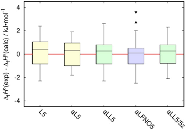
The corresponding unweighted regression results of experimental Δ_fH° via Eq. 1 using different computational schemes are given in Table 8 (deviations for individual compounds and standard deviations), Fig. 2 (deviation distributions), and Table 9 (regression coefficients). Regression covariance matrices (to be used for estimation of prediction uncertainties³) are given in Supplementary information.

Table 8:

List of compounds and deviations between experiment and calculations^a,b,c

compound	formula	(ΔfH°, exp −ΔfH°, calc)/kJ·mol−1
		L4orig	L4	aL4	aLL4	aLFNO4	L5	aL5	aLL5	aLFNO5	aLL5/5z
methane	CH4	−1.7	−1.6	−1.7	−0.7	−0.9	−1.1	−1.2	−0.9	−1.2	−0.8
ethane	C2H6	−0.3	−0.2	−0.4	0.4	0.2	0.1	−0.1	0.0	−0.2	0.2
propane	C3H8	0.2	0.2	0.1	0.8	0.7	0.4	0.3	0.2	0.1	0.4
butane	C4H10	0.4	0.4	0.5	1.1	1.1	0.4	0.5	0.4	0.4	0.4
isobutane	C4H10	−1.5	−1.5	−1.5	−0.8	−0.5	−1.5	−1.5	−1.5	−1.2	−1.5
neopentane	C5H12	−1.6	−1.6	−1.5	−0.5	0.0	−1.8	−1.6	−1.4	−0.9	−1.6
cyclohexane	C6H12	0.2	0.2	0.2	−0.2	0.0	−0.8	−0.8	−1.1	−0.8	−1.3
ethylene	C2H4	0.3	0.3	−0.1	−0.3	−0.4	1.1	0.7	1.2	1.0	1.1
propene	C3H6	0.3	0.3	0.1	−0.1	−0.1	0.9	0.7	1.3	1.2	1.3
(E)-2-butene	C4H8	−0.6	−0.6	−0.7	−0.8	−0.8	−0.1	−0.2	0.4	0.4	0.5
(Z)-2-butene	C4H8	−1.9	−1.8	−1.9	−2.0	−1.9	−1.4	−1.4	−0.8	−0.8	−0.6
cyclohexene	C6H10	0.4	0.4	0.2	−1.0	−0.8	−0.1	−0.4	0.0	0.2	0.1
norbornene	C7H10	2.6	2.5	2.4	1.5	1.7	1.2	1.0	2.4	2.7	2.3
1,3-butadiene	C4H6	−1.7	−1.7	−2.0	−2.5	−2.6	−0.8	−1.0	0.6	0.5	0.4
ethyne	C2H2	0.8	0.8	0.0	−2.0	−1.9	0.9	0.2	−0.4	−0.4	−0.5
propyne	C3H4	0.2	0.2	−0.3	−2.3	−2.2	0.1	−0.3	−0.8	−0.8	−1.0
1-butyne	C4H6	−0.7	−0.7	−1.1	−3.2	−2.9	−0.9	−1.3	−1.9	−1.6	−2.1
benzene	C6H6	1.0	0.8	0.4	−0.9	−1.0	1.3	0.8	−1.4	−1.5	−0.4
styrene	C8H8	−1.4	−1.6	−1.6	−1.9	−2.0	−1.0	−1.0	−0.8	−1.0	−0.8
naphthalene	C10H8	1.0	0.8	0.8	1.7	1.3	0.9	0.9	1.0	0.6	1.0
biphenyl	C12H10	0.9	0.6	0.7	1.3	0.7	0.9	1.0	0.4	−0.2	0.3
water	H2O	−0.3	−0.5	−0.2	0.1	−0.4	0.0	0.3	−0.1	−0.6	0.0
carbon dioxide	CO2	1.5	1.5	−0.5	−1.8	−1.7	0.9	−1.0	−1.1	−1.1	−0.9
methanol	CH4O	1.0	0.9	1.2	1.4	1.0	1.3	1.6	1.0	0.6	1.2
ethanol	C2H6O	1.0	0.9	1.2	1.3	0.9	1.1	1.4	0.8	0.4	0.9
2-propanol	C3H8O	0.8	0.7	1.0	1.2	1.1	0.7	1.0	0.6	0.5	0.5
2-methylpropan-2-ol	C4H10O	−0.2	−0.3	0.1	0.6	0.9	−0.5	−0.1	−0.3	0.1	−0.7
1-naphthol	C10H8O	−1.7	−2.0	−1.5	−0.3	−0.3	−2.0	−1.6	−1.2	−1.1	−1.1
dimethyl ether	C2H6O	0.7	0.7	1.1	1.5	1.2	0.9	1.2	0.9	0.7	1.1
anisole	C7H8O	−0.4	−0.5	−0.2	0.0	0.0	−0.4	0.0	−0.7	−0.7	−0.7
methanal	CH2O	2.1	2.2	1.5	1.1	0.8	2.4	1.8	1.7	1.4	1.6
ethanal	C2H4O	0.8	0.8	0.6	0.2	−0.1	0.9	0.7	0.7	0.4	0.7
propanone	C3H6O	0.2	0.2	0.3	0.0	0.0	0.1	0.3	0.4	0.3	0.3
formic acid	CH2O2	1.3	1.1	0.5	−0.2	−0.5	1.3	0.7	0.3	0.0	0.6
acetic acid	C2H4O2	−1.4	−1.6	−1.7	−2.6	−2.7	−1.6	−1.8	−2.2	−2.3	−1.9
benzoic acid	C7H6O2	1.6	1.3	1.3	0.4	0.7	1.2	1.3	0.5	0.8	0.6
ammonia	H3N	−0.1	−0.1	0.0	0.9	0.6	0.5	0.7	0.8	0.4	0.7
acetonitrile	C2H3N	2.4	2.6	1.6	−0.3	−0.2	2.2	1.2	0.4	0.5	0.0
urea	CH4N2O	−2.0	−2.1	−2.0	−3.0	−3.1	−1.8	−1.8	−2.3	−2.5	−1.8
piperidine	C5H11N	2.6	2.7	2.8	2.7	2.7	1.9	1.9	2.0	2.0	1.9
pyridine	C5H5N	2.0	2.1	1.3	1.2	0.8	2.1	1.3	0.8	0.5	1.1
aniline	C6H7N	0.7	0.6	0.4	0.3	0.1	1.0	0.9	−0.2	−0.4	0.2
nitrobenzene	C6H5NO2	−1.8	−1.9	−0.3	3.2	4.2	−2.3	−0.8	2.6	3.6	1.7
benzamide	C7H7NO	−1.7	−1.9	−1.7	−2.2	−1.9	−1.8	−1.6	−1.9	−1.7	−1.9
standard deviation		1.4	1.4	1.2	1.6	1.6	1.3	1.2	1.3	1.3	1.2

^aExperimental data are given in Ref. 3

^bscheme labels are defined in Table 7

^cthe vertical line separates 4- and 5-parameter schemes

Figure 2:

Distributions of deviations of Δ_fH° predicted with computational schemes (Table 7) from the experimental values. The outliers shown are: ▾ - nitrobenzene, ▴ - norbornene.

Table 9:

Regression coefficients in Eq. 1 for different computational schemes^a,b

scheme	−hi/kJ·mol−1
	C			H	O	N
	saturated	aromatic	unsaturatedc
L4orig	99 904.58			1525.78	197 129.66	143 605.53
L4	99 904.51			1525.18	197 129.65	143 605.30
aL4	99 906.82			1525.10	197 135.15	143 609.36
aLL4	99 910.30			1524.17	197 137.95	143 612.39
aLFNO4	99 910.53			1524.91	197 138.29	143 612.73
L5	99 905.32	99 904.76		1524.86	197 129.78	143 605.62
aL5	99 907.67	99 907.08		1524.77	197 135.28	143 609.70
aLL5	99 910.32		99 909.44	1524.23	197 138.05	143 612.32
aLFNO5	99 910.56		99 909.68	1524.97	197 138.39	143 612.66
aLL5/5z	99 917.56		99 916.63	1524.73	197 155.27	143 623.73

^ascheme labels are defined in Table 7

^bshaded areas indicate single atom type for multiple columns

^cother than aromatic

3.2.1. 4-parameter (atomic type) schemes

The first five schemes listed in Table 7 use the four atomic types in Eq. 1, corresponding to four elements: C, H, O, and N. Among them, the first two, “L4orig” and “L4”, are based on DLPNO-CCSD(T)/def2-QZVP energies computed using DF-MP2/def2-QZVP geometries. The only difference between them is the treatment of the ZPVE term: as discussed above, “L4” utilizes a separate frequency scaling factor. Clearly, in the context of atom-equivalent additivity (1), this does not result in noticeable changes either in standard deviation (Table 8) or in deviation distribution (Fig. 2). The next scheme, “aL4”, replaces def2-QZVP (used for geometry and single-point energy calculations in “L4”) with a larger and augmented basis set, aug-cc-pVQZ. This leads to an appreciable improvement: the standard deviation is reduced from 1.4 to 1.2 kJ·mol⁻¹ and values for some compounds improved dramatically (e.g., nitrobenzene, carbon dioxide). This is the best result obtained with 4-atomic-types scheme. Turning to other local CCSD(T) methods (LCCSD(T) and FNO-CCSD(T)) with the same basis set appears somewhat disappointing. Both LCCSD(T)-based (“aLL4”) and FNO-CCSD(T)-based (“aLFNO4”) schemes produced standard deviations that are 0.3–0.4 kJ·mol⁻¹ higher then those for all DLPNO-CCSD(T)-based schemes. This seems counter-intuitive: the evidence presented earlier (e.g., Fig. 1) suggests that FNO-CCSD(T) and LCCSD(T) are able to reproduce the canonical CCSD(T) values more closely than DLPNO-CCSD(T), especially in the atom-equivalent additivity context of Eq. 1. This strongly implies a cancellation of errors occurring in DLPNO-CCSD(T)-based schemes; in other words, the errors discussed previously are not truly uncorrelated in those cases. As an illustrative example, one can consider the case of ethyne. It shows the largest deviation from additivity for contributions beyond frozen-core CCSD(T) (−1.5 kJ·mol⁻¹), albeit among the members of very small data set (Table 1). However, ethyne’s ($\Delta E_{\text{add}}^{\text{loc}}-\Delta E^{\text{loc}}$) for DLPNO-CCSD(T) is also among the largest (1.1 kJ·mol⁻¹) and has an opposite sign (Table 3). Consequently, these two contributions nearly compensate each other, and Δ_fH° for ethyne is well-predicted by DLPNO-CCSD(T)-based methods. At the same time, ($\Delta E_{\text{add}}^{\text{loc}}-\Delta E^{\text{loc}}$) for both LCCSD(T) and FNO-CCSD(T) is only −0.1 kJ·mol⁻¹, the error cancellation does not occur, and ethyne’s Δ_fH° is overpredicted by about 2 kJ·mol⁻¹ by the schemes based on these methods (“aLL4” and “aLFNO4”). Furthermore, removal of all alkynes from the data set leads to increase in standard deviations for the DLPNO-CCSD(T)-based schemes and to decrease for those based on LCCSD(T) or FNO-CCSD(T). On the other hand, for methanal which exhibits largest positive deviation for contributions beyond frozen-core CCSD(T) (Table 1), the errors are not compensated by any local method considered.

Based on the available evidence, we can suggest that even the use of canonical CCSD(T), without any approximations, would not result in much improved performance as compared to that shown by LCCSD(T) or FNO-CCSD(T) given the present set of experimental data. However, any significant extension of this set, as discussed previously,³ is firmly constrained by the lack of experimental data of sufficient accuracy. The extent to which the error cancellation in DLPNO-CCSD(T)-based schemes can be generalized is not clear.

3.2.2. 5-parameter (atomic type) schemes

Further attempts to improve the 4-parameter scheme without additional high-level calculations would require introducing more empirical parameters. The extent of further improvements was explored by including an additional, fifth parameter in the scheme; designing more elaborate empirical schemes is not statistically justifiable.

Composite Gaussian methods introduced an empirical “higher level correction” (HLC) with the main goal to address the slow convergence of correlation energy between two spinpaired electrons with the basis set.³⁹ For closed-shell systems, this correction is proportional to the number of valence β-electrons (n_β) in the system and does not depend on atomic types explicitly, thus presenting a (potentially general) new parameter candidate. The HLC-type corrections were also reported to be beneficial in other composite methods (e.g., Ref. 40). However, within the scope of compounds considered here, n_β is reduced to a linear combination of atomic counts, n_β = 2 × n_C + (1/2) × n_H + 3 × n_O + (5/2) × n_N, where n_C, n_H, n_O, and n_N are the counts of C, H, O, and N atoms, respectively, in the system. Therefore, addition of such a term would not be useful in a context of the atom-equivalent approach, Eq. 1.

The other, although less general, possibility is to introduce atom subtypes. Among the heavy atoms considered, only carbon has representative statistical diversity in the data set. Consequently, splitting the C-atom type into two subtypes (thus increasing the total number of parameters to 5) is the only meaningful choice for this route. For each scheme, we started with four atomic subtypes for the carbon atom: saturated, aromatic, double-, and triple-bonded. The reduction of the number of subtypes was done iteratively, by merging the parameters with insignificant differences. The resulting final subtypes are defined in Table 9. For the DLPNO-CCSD(T)-based methods, the two subtypes remaining were “saturated” and “unsaturated” (including aromatic). For LCCSD(T) and FNO-CCSD(T), the subtype split was “saturated and aromatic” and “unsaturated” (other than aromatic). As previously, the results are presented in Table 8 (deviations for individual compounds and standard deviations), Fig. 2 (deviation distributions), and Table 9 (regression coefficients). The four 5-parameter schemes, “L5”, “aL5”, “aLL5”, and “aLFNO5”, are identical to their 4-parameter counterparts, with the exception of the additional regression parameter. Introduction of the additional parameter has relatively minor effect on the standard deviation for DLPNO-CCSD(T)-based methods. The span of the deviations, on the other hand, is reduced, especially for “aL5” (Fig. 2), mainly because of substantially improved values for piperidine, norbornene, and 1,3-butadiene. Formally, “aL5” is the best-performing scheme for the current data set. LCCSD(T)- and FNO-CCSD(T)-based schemes show dramatic improvement over the corresponding 4-parameter schemes, “aLL4’ and “aLFNO4”, respectively: the standard deviations for both methods were reduced from 1.6 to 1.3 kJ·mol⁻¹. Introduction of the fifth parameter clearly compensates for the lack of error cancellation exhibited by the DLPNO-CCSD(T)-based schemes and it brings these approaches to the performance comparable with that of the DLPNO-CCSD(T)-based methods. “aLFNO4”, however, exhibits two outliers, nitrobenzene and norbornene.

3.2.3. Basis set effects

Extrapolation toward complete basis set is generally considered a standard part of accurate models for thermochemical applications.²² We did not include it in our our schemes for efficiency considerations, as it requires at least one additional coupled-cluster calculation. Also, additional uncertainties associated with functional forms used for extrapolation²¹ and noise introduced by local approximations may overwhelm the advantages of considering this correction. To quantify the effect of using a finite basis set (aug-cc-pVQZ) in coupled-cluster calculations for the proposed schemes, we tested the “aLL5/5z” scheme with the single-point energy computed with the larger, aug-cc-pV5Z basis set. As seen in Table 8, the basis set upgrade does lead to a minor improvement: the standard deviation decreases from 1.3 to 1.2 kJ·mol⁻¹, mainly due to better results for benzene and nitrobenzene. However, further increase in the basis set is not likely to result in significant accuracy gains.

3.2.4. Expanded uncertainty

Based on covariance matrix analysis from our previous study, the uncertainty of predicted values is dominated by the standard deviation term for the range of molecular sizes considered here. Therefore, the expected expanded uncertainty can be estimated as twice the standard deviation given in Table 8. For the 5-parameter schemes discussed above, this results in about 2.5 kJ·mol⁻¹. This is likely close to the limit of what can be achieved with the budget semi-empirical approaches discussed in this work and the accuracy of available experimental data used for regression. Further improvements would require either computationally efficient post-CCSD(T) methods (approximations) or more empirical corrections that necessitate (presently lacking) sufficiently accurate experimental data for a set of compounds of greater diversity. For larger compounds, the errors in ZPVE are expected to become a significant contributor and efficient and accurate anharmonic ZPVE algorithms will be required to maintain the accuracy of the method.

3.2.5. Efficiency considerations

Algorithmically, all local methods considered here are comparable in computational performance, especially when set against the canonical CCSD(T) calculation. Specific performance differences are defined by the hardware configuration used and implementation preferences (MPI or OpenMP parallelization, balance between the use of memory and disk scratch space, etc.), and direct timing comparisons would be neither fair nor particularly informative. For our targeted systems (medium-sized compounds) and hardware platforms (single node with multi-core CPU, 64-1000 GB of memory, solid-state or mechanical RAID disk storage), MRCC compiled with OpenMP exhibited the best performance. The LCCSD(T)/aug-cc-pV5Z single-point energy run for the largest compound in the set, biphenyl (C₁₂H₁₀), took about 9 hours on 14 Intel Xeon E5-2697A cores with 400 GB of RAM.

3.3. Practical application

To demonstrate the utility of the proposed methodology for practical applications beyond the reference data set, we collected all new measurements of the enthalpy of formation that appeared in the most recent literature between January and July of 2018 and are within the scope of this study. This selection, although somewhat arbitrary, represents a real-life sample free of intentional bias and allows the demonstration of new data validation and resolution of experimental conflicts.

The resulting test data set includes 20 compounds and is listed in Table 10 along with the experimental Δ_fH° and the authors’-estimated expanded uncertainties. The reported uncertainties combine contributions from the condensed-state enthalpy of formation and the enthalpy of sublimation or vaporization. The set is fairly diverse with respect to molecular structural features and includes all chemical elements considered. The compounds, on average, are also larger than those included in the reference set (Table 8). It should be pointed out that one of the selection criteria for the reference set was a lack of conformational ambiguity. For the test sample, it is not the case, and the majority of compounds listed in Table 10 exhibit multiple conformations that need to be considered. Here, we adopt the model that assumes the ideal-gas equilibrium mixture of individual conformers with the entropy component of the Gibbs energy computed using the same rigid rotor-harmonic oscillator model as was used for ${\Delta }_0^{T}H$ terms. Enthalpy of formation for a given compound was computed as the Gibbs-energy average for the conformer population.

Table 10:

Comparison of recent experimental Δ_fH° with the aLL5 scheme predictions^a,b

name	CAS registry	structure	experimental		calculated
			Ref.	ΔfH°	nconf	ΔfH°(lowest)	ΔfH°(mixture)
6-methyl-1-indanone	24623-20-9		41	−95.1 ± 2.8	1	−93.0	−93.0
6-methoxy-1-indanone	13623-25-1		41	−216.0 ± 3.4	2	−215.6	−214.9
5,6-dimethoxy-1-indanone	2107-69-9		41	−356.7 ± 3.4	7	−361.9	−359.5
2-oxopropanoic acid	127-17-3		42	−535.2 ± 2.3	3	−534.3	−533.8
methyl 2-oxopropanoate	600-22-6		42	−506.4 ± 1.6	3	−506.3	−506.3
(S)-2-hydroxy-2-phenylacetic acid	17199-29-0		43	−469.0 ± 3.0	8	−471.8	−471.5
diphenyl ether	101-84-8		44	53.2 ± 2.4	2	54.9	54.9
			45	50.9 ± 1.4
methyl 2-hydroxybenzoate	119-36-8		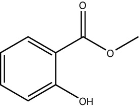46	−476.1 ± 2.8	4	−475.9	−475.8
methyl 3-hydroxybenzoate	19438-10-9		46	−452.6 ± 2.7	12	−451.6	−450.4
methyl 4-hydroxybenzoate	99-76-3		46	−454.3 ± 4.2	6	−454.2	−454.0
2-morpholinoethan-1-amine	2038-03-1		47	−144.6 ± 4.9	78	−155.9	−154.9
			c	−148.6 ± 4.9
3-morpholinopropan-1-amine	123-00-2		47	−170.1 ± 5.1	59,d	−179.3	−173.8
			c	−171.4 ± 5.1
(S)-nicotine	54-11-5		48	131.8 ± 3.0	12	132.1	132.8
2-nitrobenzamide	610-15-1		49	−99.1 ± 4.1	4	−94.7	−94.2
3-nitrobenzamide	645-09-0		49	−120.8 ± 4.0	4	−115.8	−115.1
4-nitrobenzamide	619-80-7		49	−117.0 ± 4.2	1	−113.8	−113.8
4-(2-hydroxyethyl)phenol	501-94-0		50	−302.4 ± 3.4	18	−300.0	−297.3
4-(2-hydroxyethyl)benzene-1,2-diol	10597-60-1		50	−486.3 ± 4.1	28	−478.5	−475.5
2-methylindole	95-20-5		51	123.3 ± 1.9	1	125.2	125.2
vanillin	121-33-5		52,e	−375.9 ± 1.5	8	−378.4	−377.7
			53	−378.7 ± 2.0

^aunits are kJ·mol⁻¹

^bexpanded uncertainties (0.95 level of confidence) estimated by authors are given

^cwith vaporization enthalpy corrected for water content (see text)

^dtruncated value based on mixture Δ_fH° convergence (the full list contains in excess of 200 conformers)

^eusing the enthalpy of sublimation from Ref. 53

The generation of conformers was performed with the procedure used previously.^54-57 An initial pool of conformer candidates was produced via systematic search using molecular mechanics based on MMFF94 force field.⁵⁸ The resulting conformer candidates were further optimized with B3LYP/def2-TZVP-D3(BJ) and their vibrational spectra were computed at the same level. The final set of conformers was established by eliminating duplicated structures and transition states identified from the vibrational analysis. The rotational symmetry numbers needed for the entropy evaluation were obtained using libmsym library.⁵⁹ For this test, Δ_fH° calculations were performed using only one representative (and the most efficient for our computational resources) method, the “aLL5” protocol.

The resulting number of conformers (n_conf), the lowest Δ_fH° among all conformers, and the Gibbs-energy averaged Δ_fH° are also listed in Table 10. For the majority of compounds in the test set, taking into account multiple conformations leads to under 1 kJ·mol⁻¹ difference in Δ_fH° as compared to the corresponding value for the most stable conformer. For four compounds, however, this difference exceeds 2 kJ·mol⁻¹ (up to 5.5 kJ·mol⁻¹ for highly flexible 3-morpholinopropan-1-amine). The deviations between the experimental and computed Δ_fH° are shown in Fig. 3. Overall, the predictions are in excellent agreement with the experimental data, and, for the majority of compounds in the data set, the deviations are within the uncertainty. For two compounds, diphenyl ether and vanillin, there are independent measurements from different groups. For vanillin, the measurements of Maksimuk et al.⁵² and Almeida et al.⁵³ are in agreement with each other and the present computational result. For diphenyl ether, our calculations are in agreement with the results of Lukyanova et al.,⁴⁴ while the value reported by Emel’yanenko et al.⁴⁵ is about 4 kJ·mol⁻¹ lower and slightly outside of the uncertainty bounds. A similar deviation (3.2 to 5.7 kJ·mol⁻¹) is observed for nitrobenzamides studied in the same laboratory,⁴⁹ although the experimental uncertainties in that case are higher.

Figure 3:

Deviations between the experimental and computed Δ_fH° for the test set of compounds listed in Table 10. The errorbars represent experimental uncertainties and the shaded area indicates the estimated uncertainty of the computational scheme used (aLL5).

In spite of the overall very good agreement between the experiment and the computations, there are two prominent outliers in the data set: 2-morpholinoethan-1-amine and 4-(2-hydroxyethyl)benzene-1,2-diol. Both compounds are highly hygroscopic, and the observed deviations may be attributed to a common problem associated with the presence of water in the studied samples that was not accounted for in data analysis. For these two compounds, the condensed-phase Δ_fH° was determined from their energies of combustion measured in bomb calorimeters. In addition, the enthalpy of vaporization (for 2-morpholinoethan-1-amine) and sublimation (for 4-(2-hydroxyethyl)benzene-1,2-diol) were measured, also calorimetrically, to obtain the gas-phase Δ_fH° from the condensed-phase Δ_fH°. The presence of water affects both the condensed-phase Δ_fH° (decrease) and the enthalpy of vaporization/sublimation (increase). The effect of water on the condensed-phase Δ_fH° typically dominates the resulting value of the gas-phase Δ_fH°.

For 2-morpholinoethan-1-amine, the average CO₂ yield in the combustion products is 0.984 of the theoretical value,⁴⁷ which was attributed to the presence of water. Notably, for a similar compound studied in the same work, 3-morpholinopropan-1-amine, CO₂ yield was much closer to 1 (0.9954), and the reported experimental value is in agreement with the computations within the uncertainty. In the original analysis,⁴⁷ the traces of water were taken into account for the energy of combustion, but were not considered in derivation of the enthalpy of vaporization. Consequently, the resulting gas-phase Δ_fH° is expected to be overestimated due to increased enthalpy of vaporization, in consistence with the observed deviation from the calculations (Fig. 3). Including a rough estimate of the effect of water on the enthalpy of vaporization (assuming ideal solution behavior of the components) leads to substantially improved agreement with the computations for 2-morpholinoethan-1-amine and 3-morpholinopropan-1-amine (Table 10).

For 4-(2-hydroxyethyl)benzene-1,2-diol, the water content was not determined⁵⁰ and was not considered in the data analysis. Therefore, if water was indeed present in the sample, one would expect the gas-phase Δ_fH° to be underestimated due to the main effect of water on the condensed-phase Δ_fH°. This is, again, consistent with our calculations (Fig. 3). To explain the observed deviation between the experiment and the calculations, the sample should have a water content of several mole percent. This level of impurities, in turn, is supported by Differential Scanning Calorimetry (DSC) curves reported in Fig. S1 of the original publication:⁵⁰ the pre-melting of 4-(2-hydroxyethyl)benzene-1,2-diol sample starts at about 50 K below its melting temperature.

4. Conclusions

Building upon the encouraging performance of the atom-equivalent-type schemes based on a local CCSD(T) approximation for prediction of the enthalpies of formation for closed-shell organic compounds demonstrated in our previous study,³ we presented a further investigation of this idea, systematically exploring its limitations and possibilities for improvement. Analysis of neglected energy contributions beyond frozen-core CCSD(T) and errors introduced by the local CCSD(T) and scaled harmonic ZPVE approximations demonstrates that the expanded uncertainty of the proposed approach is generally limited to about 2 kJ·mol⁻¹. Investigation of three local CCSD(T) methods, DLPNO-CCSD(T), LCCSD(T), and FNO-CCSD(T), shows that, with atom-equivalent-type corrections, they are able to reproduce the canonical CCSD(T) values with standard deviations of 0.7, 0.2, and 0.1 kJ·mol⁻¹, respectively. The 4-parameter computational scheme based on DLPNO-CCSD(T)/aug-cc-pVQZ energies predicts the enthalpies of formation with an estimated expanded uncertainty of about 2.4 kJ·mol⁻¹. Further analysis suggests that this accuracy is achieved by the cancellation of errors due to neglect of post-CCSD(T) contributions and deviation from the canonical CCSD(T) for some problematic compounds, which is not observed for the other local methods. Extended, 5-parameter schemes exhibit similar performance across all three local CCSD(T) methods with an estimated expanded uncertainty of about 2.5 kJ·mol⁻¹, approaching the levels of the most accurate calorimetric measurements and improving upon the previous results.³ A combination of computational efficiency and accuracy offers unprecedented advantages for practical applications, including large-scale evaluations and resolution of long-standing experimental conflicts. This was further demonstrated using a test data set collected from the most recent literature. Extensions of the proposed schemes to other elements of practical interest, such as sulfur and halogens, are planned in the future.

References

- (1).Pedley JB Thermochemical Data and Structures of Organic Compounds; TRC Data Series; Thermodynamics Research Center, College Station, TX, 1994. [Google Scholar]
- (2).Irikura KK In Energetics of Stable Molecules and Reactive Intermediates; Minas da Piedade ME, Ed.; Kluwer Academic Publishers, Dordrecht, the Netherlands, 1999; pp 353–372. [Google Scholar]
- (3).Paulechka E; Kazakov A Efficient DLPNO-CCSD(T)-based estimation of formation enthalpies for C-, H-, O-, and N-containing closed-shell compounds validated against critically evaluated experimental data. J. Phys. Chem. A 2017, 121, 4379–4387. [DOI] [PMC free article] [PubMed] [Google Scholar]
- (4).Raghavachari K; Stefanov BB; Curtiss LA Accurate thermochemistry for larger molecules: Gaussian-2 theory with bond separation energies. J. Chem. Phys 1997, 106, 6764–6767. [Google Scholar]
- (5).Riplinger C; Neese F An efficient and near linear scaling pair natural orbital based local coupled cluster method. J Chem. Phys 2013, 138, 034106. [DOI] [PubMed] [Google Scholar]
- (6).Riplinger C; Sandhoefer B; Hansen A; Neese F Natural triple excitations in local coupled cluster calculations with pair natural orbitals. J. Chem. Phys 2013, 139, 134101. [DOI] [PubMed] [Google Scholar]
- (7).DePrince III AE; Sherrill CD Accuracy and Efficiency of Coupled-Cluster Theory Using Density Fitting/Cholesky Decomposition, Frozen Natural Orbitals, and a t1-Transformed Hamiltonian. J. Chem. Theory Comput 2013, 9, 2687–2696. [DOI] [PubMed] [Google Scholar]
- (8).Nagy PR; Kállay M Optimization of the linear-scaling local natural orbital CCSD(T) method: Redundancy-free triples correction using Laplace transform. J. Chem. Phys 2017, 146, 214106. [DOI] [PMC free article] [PubMed] [Google Scholar]
- (9).Nagy PR; Samu G; Kállay M An Integral-Direct Linear-Scaling Second-Order Møller-Plesset Approach. J. Chem. Theory Comput 2016, 12, 4897–4914. [DOI] [PubMed] [Google Scholar]
- (10).Kállay M; Rolik Z; Csontos J; Nagy P; Samu G; Mester D; Csóka J; Szabó B; Ladjánszki I; Szegedy L; Ladóczki B; Petrov K; Farkas M; Mezei PD; Hégely B Mrcc, a quantum chemical program suite. http://www.mrcc.hu, 2017. [DOI] [PubMed] [Google Scholar]
- (11).Weigend F; Ahlrichs R Balanced basis sets of split valence, triple zeta valence and quadruple zeta valence quality for H to Rn: Design and assessment of accuracy. Phys. Chew. Chew. Phys 2005, 7, 3297–3305. [DOI] [PubMed] [Google Scholar]
- (12).Dunning TH Jr Gaussian basis sets for use in correlated molecular calculations. I. The atoms boron through neon and hydrogen. J. Chem. Phys 1989, 90, 1007–1023. [Google Scholar]
- (13).Kendall RA; Dunning TH Jr; Harrison RJ Electron affinities of the first-row atoms revisited. Systematic basis sets and wave functions. J. Chem. Phys 1992, 96, 6796–6806. [Google Scholar]
- (14).Jensen F Polarization consistent basis sets: Principles. J. Chem. Phys 2001, 115, 9113–9125. [Google Scholar]
- (15).Jensen F Polarization consistent basis sets. III. The importance of diffuse functions. J. Chem. Phys 2002, 117, 9234–9240. [Google Scholar]
- (16).Peverati R; Truhlar DG Exchange-Correlation Functional with Good Accuracy for Both Structural and Energetic Properties while Depending Only on the Density and Its Gradient. J. Chem. Theory Comput 2012, 8, 2310–2319. [DOI] [PubMed] [Google Scholar]
- (17).Chan B Use of Low-Cost Quantum Chemistry Procedures for Geometry Optimization and Vibrational Frequency Calculations: Determination of Frequency Scale Factors and Application to Reactions of Large Systems. J. Chem. Theory Comput 2017, 13, 6052–6060. [DOI] [PubMed] [Google Scholar]
- (18).Frisch MJ; Trucks GW; Schlegel HB; Scuseria GE; Robb MA; Cheeseman JR; Scalmani G; Barone V; Mennucci B; Petersson GA; Nakatsuji H; Caricato M; Li X; Hratchian HP; Izmaylov AF; Bloino J; Zheng G; Sonnenberg JL; Hada M; Ehara M; Toyota K; Fukuda R; Hasegawa J; Ishida M; Nakajima T; Honda Y; Kitao O; Nakai H; Vreven T; Montgomery JA Jr.; Peralta JE; Ogliaro F; Bearpark M; Heyd JJ; Brothers E; Kudin KN; Staroverov VN; Keith T; Kobayashi R; Normand J; Raghavachari K; Rendell A; Burant JC; Iyengar SS; Tomasi J; Cossi M; Rega N; Millam JM; Klene M; Knox JE; Cross JB; Bakken V; Adamo C; Jaramillo J; Gomperts R; Stratmann RE; Yazyev O; Austin AJ; Cammi R; Pomelli C; Ochterski JW; Martin RL; Morokuma K; Zakrzewski VG; Voth GA; Salvador P; Dannenberg JJ; Dapprich S; Daniels AD; Farkas O; Foresman JB; Ortiz JV; Cioslowski J; Fox DJ Gaussian 09 Revision D.01. Gaussian Inc, Wallingford CT, 2013. [Google Scholar]
- (19).Parrish RM; Burns LA; Smith DGA; Simmonett AC; DePrince AE; Hohenstein EG; Bozkaya U; Sokolov AY; Di Remigio R; Richard RM; Gonthier JF; James AM; McAlexander HR; Kumar A; Saitow M; Wang X; Pritchard BP; Verma P; Schaefer HF; Patkowski K; King RA; Valeev EF; Evangelista FA; Turney JM; Crawford TD; Sherrill CD Psi4 1.1: An Open-Source Electronic Structure Program Emphasizing Automation, Advanced Libraries, and Interoperability. J. Chem. Theory Comput 2017, 13, 3185–3197. [DOI] [PMC free article] [PubMed] [Google Scholar]
- (20).Neese F The ORCA program system. Wiley Interdiscip. Rev.: Comput. Mol. Sci 2012, 2, 73–78. [Google Scholar]
- (21).Martin JML In Energetics of Stable Molecules and Reactive Intermediates; Minas da Piedade ME, Ed.; Kluwer Academic Publishers, Dordrecht, the Netherlands, 1999; pp 373–415. [Google Scholar]
- (22).Karton A A computational chemist’s guide to accurate thermochemistry for organic molecules. Wiley Interdiscip. Rev.: Comput. Mol. Sci 2016, 6, 292–310. [Google Scholar]
- (23).Karton A; Rabinovich E; Martin JML; Ruscic B W4 theory for computational thermochemistry: In pursuit of confident sub-kJ/mol predictions. J. Chem. Phys 2006, 125, 144108. [DOI] [PubMed] [Google Scholar]
- (24).Karton A; Gruzman D; Martin JML Benchmark Thermochemistry of the CnH2n+2 Alkane Isomers (n = 2 – 8) and Performance of DFT and Composite Ab Initio Methods for Dispersion-Driven Isomeric Equilibria. J. Phys. Chem. A 2009, 113, 8434–8447. [DOI] [PubMed] [Google Scholar]
- (25).Harding ME; Vázquez J; Gauss J; Stanton JF; Kállay M Towards highly accurate ab initio thermochemistry of larger systems: Benzene. J. Chem. Phys 2011, 135, 044513. [DOI] [PubMed] [Google Scholar]
- (26).Sylvetsky N; Peterson KA; Karton A; Martin JM Toward a W4-F12 approach: Can explicitly correlated and orbital-based ab initio CCSD(T) limits be reconciled? J. Chem. Phys 2016, 144, 214101. [DOI] [PubMed] [Google Scholar]
- (27).Karton A How large are post-CCSD(T) contributions to the total atomization energies of medium-sized alkanes? Chem. Phys. Lett 2016, 645, 118–122. [Google Scholar]
- (28).Liakos DG; Sparta M; Kesharwani MK; Martin JML; Neese F Exploring the Accuracy Limits of Local Pair Natural Orbital Coupled-Cluster Theory. J. Chem. Theory Comput 2015, 11, 1525–1539. [DOI] [PubMed] [Google Scholar]
- (29).Riplinger C; Pinski P; Becker U; Valeev EF; Neese F Sparse maps – A systematic infrastructure for reduced-scaling electronic structure methods. II. Linear scaling domain based pair natural orbital coupled cluster theory. J. Chem. Phys 2016, 144, 024109. [DOI] [PubMed] [Google Scholar]
- (30).Merrick JP; Moran D; Radom L An Evaluation of Harmonic Vibrational Frequency Scale Factors. J. Phys. Chew. A 2007, 111, 11683–11700. [DOI] [PubMed] [Google Scholar]
- (31).Grev RS; Janssen CL; Schaefer III HF Concerning zero-point vibrational energy corrections to electronic energies. J. Chem. Phys 1991, 95, 5128–5132. [Google Scholar]
- (32).Pfeiffer F; Rauhut G; Feller D; Peterson KA Anharmonic zero point vibrational energies: Tipping the scales in accurate thermochemistry calculations? J. Chem. Phys 2013, 138, 044311. [DOI] [PubMed] [Google Scholar]
- (33).Harding LB; Georgievskii Y; Klippenstein SJ Accurate anharmonic zero-point energies for some combustion-related species from diffusion Monte Carlo. J. Phys. Chew. A 2017, 121, 4334–4340. [DOI] [PubMed] [Google Scholar]
- (34).Barone V Vibrational zero-point energies and thermodynamic functions beyond the harmonic approximation. J. Chem. Phys 2004, 120, 3059–3065. [DOI] [PubMed] [Google Scholar]
- (35).Barone V Anharmonic vibrational properties by a fully automated second-order perturbative approach. J. Chem. Phys 2005, 122, 014108. [DOI] [PubMed] [Google Scholar]
- (36).Császár AG; Furtenbacher T Zero-cost estimation of zero-point energies. J. Phys. Chem. A 2015, 119, 10229–10240. [DOI] [PubMed] [Google Scholar]
- (37).Kesharwani MK; Brauer B; Martin JML Vibrational Energy Scale Factors for Double-Hybrid Density Functionals (and Other Selected Methods): Can Anharmonic Force Fields Be Avoided? J. Phys. Chem. A 2015, 119, 1701–1714. [DOI] [PubMed] [Google Scholar]
- (38).Dorofeeva OV; Ryzhova ON Enthalpy of Formation and O-H Bond Dissociation Enthalpy of Phenol: Inconsistency between Theory and Experiment. J. Phys. Chem. A 2016, 120, 2471–2479. [DOI] [PubMed] [Google Scholar]
- (39).Pople JA; Head-Gordon M; Fox DJ; Raghavachari K; Curtiss LA Gaussian-1 theory: A general procedure for prediction of molecular energies. J. Chem. Phys 1989, 90, 5622–5629. [Google Scholar]
- (40).Chan B Unification of the W1X and G4(MP2)-6X Composite Protocols. J. Chem. Theory Comput 2017, 13, 2642–2649. [DOI] [PubMed] [Google Scholar]
- (41).Silva ALR; Lima ACMO; da Silva MDMCR Energetic characterization of indanone derivatives involved in biomass degradation. J. Therm. Anal. Calorim 2018, 10.1007/s10973-018-7533-z. [DOI] [Google Scholar]
- (42).Emel’yanenko VN; Turovtsev VV; Fedina YA Thermodynamic properties of pyruvic acid and its methyl ester. Thermochim. Acta 2018, 665, 70–75. [Google Scholar]
- (43).Emel’yanenko VN; Turovtsev VV; Fedina YA Experimental and theoretical thermodynamic properties of RS-(±)- and S-(+)-mandelic acids. Thermochim. Acta 2018, 665, 37–42. [Google Scholar]
- (44).Lukyanova V; Pimenova S; Druzhinina A; Tarazanov S; Dorofeeva O Standard enthalpy of formation of diphenyl oxide. J. Chem. Thermodyn 2018, 124, 43–48. [Google Scholar]
- (45).Emel’yanenko VN; Zaitsau DH; Pimerzin AA; Verevkin SP Benchmark properties of diphenyl oxide as a potential liquid organic hydrogen carrier: Evaluation of thermochemical data with complementary experimental and computational methods. J. Chem. Thermodyn 2018, 125, 149–158. [Google Scholar]
- (46).Ledo JM; Flores H; Solano-Altamirano J; Ramos F; Hernández-Pérez JM; Camarillo EA; Rabell B; Amador MP Experimental and theoretical study of methyl n-hydroxybenzoates. J. Chem. Thermodyn 2018, 124, 1–9. [Google Scholar]
- (47).Freitas VL; Silva CA; da Silva MDR Energetic vs structural effects of aminoalkyl substituents in the morpholine. J. Chem. Thermodyn 2018, 122, 95–101. [Google Scholar]
- (48).Emel’yanenko VN; Turovtsev VV; Fedina YA; Sikorski P Thermodynamic properties of S-(−)-nicotine. J. Chem. Thermodyn 2018, 120, 97–103. [Google Scholar]
- (49).Verevkin SP; Emel’yanenko VN; Zaitsau DH Thermochemistry of Substituted Benzamides and Substituted Benzoic Acids: Like Tree, Like Fruit? ChemPhysChem 2018, 19, 619–630. [DOI] [PubMed] [Google Scholar]
- (50).Dávalos JZ; Valderrama-Negrón AC; Barrios JR; Freitas VLS; da Silva MDMCR Energetic and Structural Properties of Two Phenolic Antioxidants: Tyrosol and Hydroxytyrosol. J. Phys. Chem. A 2018, 122, 4130–4137. [DOI] [PubMed] [Google Scholar]
- (51).Chirico RD; Paulechka E; Bazyleva A; Kazakov AF Thermodynamic properties of 2-methylindole: Experimental and computational results for gas-phase entropy and enthalpy of formation. J. Chem. Thermodyn 2018, 125, 257–270. [Google Scholar]
- (52).Maksimuk Y; Ponomarev D; Sushkova A; Krouk V; Vasarenko I; Antonava Z Standard molar enthalpy of formation of vanillin. J. Therm. Anal. Calorim 2018, 131, 1721–1733. [Google Scholar]
- (53).Almeida AR; Freitas VL; Campos JI; da Silva MDR; Monte MJ Volatility and thermodynamic stability of vanillin. J. Chem. Thermodyn 2019, 128, 45–54. [Google Scholar]
- (54).Kazakov A; Muzny CD; Diky V; Chirico RD; Frenkel M Predictive correlations based on large experimental datasets: Critical constants for pure compounds. Fluid Phase Equilib. 2010, 298, 131–142. [Google Scholar]
- (55).Kazakov A; McLinden MO; Frenkel M Computational Design of New Refrigerant Fluids Based on Environmental, Safety, and Thermodynamic Characteristics. Ind. Eng. Chew,. Res 2012, 51, 12537–12548. [Google Scholar]
- (56).Paulechka E; Diky V; Kazakov A; Kroenlein K; Frenkel M Reparameterization of COSMO-SAC for Phase Equilibrium Properties Based on Critically Evaluated Data. J. Chem. Eng. Data 2015, 60, 3554–3561. [Google Scholar]
- (57).Carande WH; Kazakov A; Muzny C; Frenkel M Quantitative Structure-Property Relationship Predictions of Critical Properties and Acentric Factors for Pure Compounds. J. Chem. Eng. Data 2015, 60, 1377–1387. [Google Scholar]
- (58).Halgren TA Merck molecular force field. I. Basis, form, scope, parameterization, and performance of MMFF94. J. Comput. Chew 1996, 17, 490–519. [Google Scholar]
- (59).Johansson M; Veryazov V Automatic procedure for generating symmetry adapted wavefunctions. J. Cheminf 2017, 9, 8. [DOI] [PMC free article] [PubMed] [Google Scholar]
Associated Data
This section collects any data citations, data availability statements, or supplementary materials included in this article.