Relationships Between Supermicrometer Sea Salt Aerosol and Marine Boundary Layer Conditions: Insights From Repeated Identical Flight Patterns

Abstract

The MONterey Aerosol Research Campaign (MONARC) in May–June 2019 featured 14 repeated identical flights off the California coast over the open ocean at the same time each flight day. The objective of this study is to use MONARC data along with machine learning analysis to evaluate relationships between both supermicrometer sea salt aerosol number (N_>1) and volume (V_>1) concentrations and wind speed, wind direction, sea surface temperature (SST), ambient temperature (T_amb), turbulent kinetic energy (TKE), relative humidity (RH), marine boundary layer (MBL) depth, and drizzle rate. Selected findings from this study include the following: (i) Near surface (<60 m) N_>1 and V_>1 concentration ranges were 0.1–4.6 cm⁻³ and 0.3–28.2 μm³ cm⁻³, respectively; (ii) four meteorological regimes were identified during MONARC with each resulting in different N_>1 and V_>1 concentrations and also varying horizontal and vertical profiles; (iii) the relative predictive strength of the MBL properties varies depending on predicting N_>1 or V_>1, with MBL depth being more highly ranked for predicting N_>1 and with TKE being higher for predicting V_>1; (iv) MBL depths >400 m (<200 m) often correspond to lower (higher) N_>1 and V_>1 concentrations; (v) enhanced drizzle rates coincide with reduced N_>1 and V_>1 concentrations; (vi) N_>1 and V_>1 concentrations exhibit an overall negative relationship with SST and RH and an overall positive relationship with T_amb; and (vii) wind speed and direction were relatively weak predictors of N_>1 and V_>1.

1. Introduction

The marine boundary layer (MBL) contains a diverse population of supermicrometer (particle diameter [D_p] > 1 μm) aerosol types, from primary biological particles and sea salt to entrained continental particle types such as soil dust and ash (Kelly et al., 2007; Radke et al., 1988) and potentially even ship exhaust (Sorooshian et al., 2015). Of great importance are sea salt aerosol (SSA) particles emitted from the surface of the ocean, which have been linked to the largest mass emission flux of all aerosol types (Andreae & Rosenfeld, 2008). SSA particles significantly impact the earth’s energy budget (Collins et al., 2000; Fei et al., 2019; Haywood et al., 1999; Murphy et al., 1998; Partanen et al., 2014; Takemura et al., 2000), interact with clouds (Beard & Ochs, 1993; Dadashazar et al., 2017; Dong et al., 2015; Feingold et al., 1999; Johnson, 1982; Jung et al., 2015; Woodcock, 1952), and both drive geochemical cycles (Boyce, 1954; Keene et al., 2017; Monahan, 1968) and participate in chemical reactions with gases that can liberate species such as chloride and bromide (Braun et al., 2017; Graedel & Keene, 1995; Haskins et al., 2019; Skartveit, 1982; Zhou et al., 2005). The inability to accurately simulate the horizontal and vertical distribution of SSA particles limits the ability to forecast their impacts in the MBL such as on cloud properties and radiative transfer (Fei et al., 2019).

There are significant differences in results from general circulation models (GCMs) for the life cycle of SSA (e.g., emissions, transport, and deposition), with model diversity reaching up to 199% for SSA emissions (Textor et al., 2006). Keene et al. (2017) provide an especially comprehensive summary of the confounders of SSA production at the ocean-air interface, which impact the concentrations of these particles in the MBL, the latter of which is the focus of this study. It is generally agreed that SSA particles are injected into the atmosphere by bursting of bubbles at the ocean surface and then transported by surface-level winds (Andreas, 1998). However, only a fraction of the near surface SSA mass concentration in the MBL can be explained by wind speed alone (Hanley et al., 2010; Reid et al., 2001). Various aspects of SSA particles (e.g., horizontal and vertical profiles and fluxes) in the MBL have also been noted to be influenced by sea surface temperature (SST) (Jaeglé et al., 2011; Salter et al., 2015), MBL stability (Monahan et al., 1986; Stramska & Petelski, 2003), wave kinematics (Lenain & Melville, 2017; Zhao & Toba, 2001), ocean salinity (Sofiev et al., 2011; Zábori et al., 2012), drizzle rate (Dana & Hales, 1976; Skartveit, 1982), MBL depth (Lewis & Schwartz, 2004), and the synoptic scale air path (i.e., fetch) (Wu, 1975). The degree to which any of the above conditions influence atmospheric SSA fluxes and number concentration varies between independent studies (Barthel et al., 2019; Veron, 2015; Veron et al., 2012).

While dry SSA particle diameters range from tens of nanometers to greater than 100 μm (Andreae & Rosenfeld, 2008; Keene et al., 2007; Lewis & Schwartz, 2004; Mårtensson et al., 2003), supermicrometer SSA (hereafter referred to as SM-SSA) particles are of special interest in this study as they can account for ~94% of the global atmospheric SSA mass burden and ~61% of the global aerosol optical depth (AOD) burden (Fei et al., 2019). Furthermore, the impacts of these larger particles extend to clouds since they are sufficiently large to serve as giant cloud condensation nuclei (GCCN) (Feingold et al., 1999; Johnson, 1982; Kogan et al., 2012). In certain conditions associated with the amount of cloud liquid water and background pollution levels (Cheng et al., 2009; Dagan et al., 2015; Feingold et al., 1999; Teller & Levin, 2006), GCCN can broaden cloud droplet size distributions, leading to larger droplets and faster onset of warm drizzle (L’Ecuyer et al., 2009). Airborne measurements have confirmed that the presence of GCCN, even at very small concentrations (~10⁻⁴ to 10⁻² cm⁻³), can significantly enhance drizzle rate in marine stratocumulus (Sc) clouds (Jung et al., 2015). The very largest sea spray droplets include spume droplets that have diameters generally exceeding 40 μm (Veron et al., 2012). These droplets play a significant role in exchanging momentum with the wind and are important for air-sea heat fluxes (Andreas, 1992). Spume drops are produced when water is removed off of wave crests at higher wind speeds (>7–11 m s⁻¹) (Andreas, 1995; Veron, 2015).

There have been only a few airborne studies that have directly measured vertical and horizontal distributions of SM-SSA concentrations within the MBL with the intent of probing the physical processes that control those distributions (e.g., Lenain & Melville, 2017; Murphy et al., 2019; Reid et al., 2001). Aircraft measurements offer the benefit of (i) providing vertically resolved boundary layer information with high spatial and temporal resolution, (ii) offering insight into factors that are related to SM-SSA concentration and associated spatial distribution, and (iii) helping to validate findings from laboratory and modeling studies. Aside from intercomparing SM-SSA levels with other MBL properties in the form of scatterplots, machine learning regression (MLR) algorithms are also applied in this study, which can make predictions given highly complex and nonlinear systems. MLR has been applied to a range of complex systems, such as for interpretation of mass spectroscopy data (Christopoulos et al., 2018; Marsden et al., 2019), studies of aerosol mixing states using GCMs (Hughes et al., 2018), and studies related to weather prediction models (Feng et al., 2018). MLR offers the opportunity to indirectly probe physical processes influencing their concentrations without the constraints of theory-based frameworks that have failed to provide consensus on concentrations and spatial distributions.

The MONterey Aerosol Research Campaign (MONARC) in May–June 2019 involved repeating identical flight paths off the California coast at the same time each flight day to measure 2-D profiles of SM-SSA particles. This statistical approach of airborne data collection provided a data set that could be tested with MLR techniques to determine what MBL properties were most influential for predicting near surface (<60 m) SM-SSA particle concentrations. The goal of this study is to use the MONARC data to address the following questions: (i) What was the meteorological backdrop during the MONARC campaign and how did the SM-SSA number and volume concentrations vary in different meteorological regimes encountered?; (ii) how were SM-SSA particles distributed within the MBL, both vertically and horizontally with respect to offshore distance, under varying MBL conditions?; (iii) how are MBL conditions related to SM-SSA number and volume concentrations, especially at the near surface level?; and (iv) how well can MLR models predict near surface SM-SSA number and volume concentrations? The results of this study have implications for general understanding of the nature of SM-SSA particle concentrations in the MBL for all oceanic areas and for demonstrating the utility of the flight approach taken for future field studies. Note also that while we hereafter reference SM-SSA concentrations, our results do not preclude the possibility that other aerosol types such as biological particles contribute to the concentrations reported here.

2. Methods

2.1. Field Campaign Description and Flight Strategy

MONARC was carried out between 28 May and 14 June 2019 using the Center for Remotely-Piloted Aircraft Studies (CIRPAS) Twin Otter aircraft. The MONARC had a total of ~70 flight hours spread across 14 research flights (RFs) based out of Marina, California, and with sampling conducted off the coast over the northeastern Pacific Ocean. Table 1 summarizes pertinent details of each RF, including dates, times, and the “turnaround point” time, which will be described below. The MONARC flights were designed to be as repetitive as possible to ensure that flight-to-flight comparisons could be done meaningfully in a statistical way. Similarly, comparisons were possible at each point along the flight path at two times on a particular day.

Table 1.

Flight Date, Takeoff and Landing Times (UTC), and Latitude and Longitude of the Turnaround Point (Most Western Point) for Each Research Flight (RF) in the MONARC

RF	Date	Takeoff	Landing	Lat (°N)	Lon (°E)
1	05/28/2019	20:12:30	23:51:35	37.29	−125.33
2	05/29/2019	17:39:32	22:20:00	37.45	−126.41
3	05/30/2019	17:36:43	22:21:32	37.46	−126.55
4	05/31/2019	17:43:32	22:19:01	37.42	−126.25
5	06/03/2019	17:42:03	22:22:54	37.46	−126.53
6	06/04/2019	17:51:22	22:50:18	37.47	−126.70
7	06/05/2019	17:36:49	22:44:14	37.49	−126.69
8	06/06/2019	17:47:19	23:02:25	37.47	−126.69
9	06/07/2019	17:09:31	22:23:50	37.49	−126.70
10	06/10/2019	17:31:59	22:14:13	37.49	−126.71
11	06/11/2019	17:35:25	22:21:27	37.49	−126.71
12	06/12/2019	17:27:12	22:32:01	37.49	−126.72
13	06/13/2019	17:25:47	22:23:48	37.49	−126.74
14	06/14/2019	17:45:48	22:54:57	37.49	−126.72

Note. Dates are formatted as MM/DD/YYYY.

Each RF involved following a straight path from Marina Airport to a point as far as possible offshore to the west given fuel limitations and then following the same path back to Marina Airport. Figure 1 shows both the 2-D flight paths for all the MONARC RFs and separately the 3-D path for RF14 as a representation of the “cycle” method employed each RF. During the straight paths to and from Marina, the Twin Otter went through repetitive stair-stepping cycles involving a series of different level legs varying in altitude both below and above the top of the MBL. The steps involved for each cycle were as follows: near surface leg (~30 m altitude and always <60 m), below-cloud leg (just below cloud-base), cloud-base leg (just above cloud-base), cloud-mid leg (midpoint between cloud-top and cloud-base), cloud-top leg (just below cloud-top), wheels-in leg (just above cloud-top with aircraft wheels roughly skimming cloud tops), above-cloud leg (150 m above cloud-top), and lastly a descent down to the near surface level to repeat the cycle. The altitudes of all legs, except for the near surface leg, were set based on the cloud-base and cloud-top altitudes. In RFs where no clouds were present, the altitude at the top of the MBL was used to set approximate altitudes for each leg, with three legs still below the MBL top and at least two above it. The typical time duration for a given cycle was between 10 and 40 min, with 11 to 14 cycles usually conducted per ~5 h flight.

Figure 1.

(a) Flight paths for all research flights (RFs) during the MONARC and (b) a three-dimensional profile of a representative flight (RF14 on 14 June 2019), which was similar for all flights. The blue (orange) trace in (b) is for the first (second) half of the flight.

At the “turnaround point” for each RF, which was the farthest west point of the flight (~300 to 400 km offshore), the Twin Otter would perform a downward spiral down to the near surface level. This spiral was always initiated at the end of the above cloud leg (150 m above tops) and would last approximately ~12 min.

2.2. Instrumentation

The Twin Otter carried a myriad of instruments in order to track position and measure a suite of atmospheric parameters related to meteorology, aerosols, and clouds. For a complete list and detailed description of all the instrumentation carried by the Twin Otter along with quality control/assurance steps, refer to Sorooshian et al. (2018). A short summary of the instruments used in this study is provided here.

The navigational and meteorological systems on the Twin Otter measure aircraft position (latitude/longitude and altitude), barometric pressure (pressure altitude), horizontal and vertical wind velocities, ambient temperature (T_amb), skin surface temperature, and aircraft true air speed. Measurements of skin surface temperature are taken in this study to be equivalent to SST as we use data only when collected at an altitude less than 60 m to prevent any cloud interference and to maximize getting a measurement of the ocean surface rather than the cloud surface (Sorooshian et al., 2018). The Twin Otter has a set of wing-mounted aerosol and cloud sampling probes to characterize aerosol and cloud droplet size distributions. The probes relevant to this study include the Cloud, Aerosol, and Precipitation Spectrometer (CAPS; Droplet Measurement Technologies, Inc.), which contains both the cloud and aerosol spectrometer (CAS) and the cloud imaging probe (CIP). The CAS measures aerosol and droplet size distributions for the ambient D_p range between 0.76 and 75.80 μm.

Because the CAS samples aerosol under ambient relative humidity (RH) conditions, the dry D_p range of each CAS size bin had to be calculated. To do this, the D_p at ambient RH conditions was first converted to D_p at RH = 80% by using the growth factor parameterization presented by Lewis and Schwartz (2004). Note that other parameterizations exist such as that of Zieger et al. (2017); however, based on sensitivity calculations, the percent error for dry D_p values based on the ambient D_p range between 3 and 10 μm at 90% RH is ≤3% between the two methods. Thus, the conclusions reached here are preserved regardless of which of the two parameterization methods are used. Following Lewis and Schwartz (2004) and Jaeglé et al. (2011), the dry D_p was subsequently calculated by dividing the D_p at RH = 80% by two. The SM-SSA number and volume concentrations, referred to hereafter as N_>1 and V_>1, respectively, were calculated using CAS size bins where the calculated minimum dry D_p was ≥1 μm. The range observed for the upper bound of dry D_p for the SM-SSA distributions varied between 14 and 63 μm.

The CIP measures droplet and raindrop number concentrations for the D_p range between 25 and 1,550 μm. The CIP is used to calculate cloud-base drizzle rate (r_cb) which is calculated using the lower third of clouds. A PVM-100A probe was additionally used to measure liquid water content (LWC) using light diffraction (Gerber et al., 1994).

A cloud water collector was manually protruded out of the fuselage roof when sampling in cloud (Hegg & Hobbs, 1986). Cloud water samples collected during each RF were analyzed using ion chromatography (IC; Thermo Scientific Dionex ICS-2100 system). Of relevance to this study was the measurement of Na⁺, which is used here as a tracer for SSA. In contrast, Cl⁻ (the major component of SSA by mass) is vulnerable to well-documented depletion reactions in the region (Braun et al., 2017). The reader is referred to past works for more detailed explanation of the cloud water collection and analysis details (MacDonald et al., 2018; Wang et al., 2014; Wang et al., 2016). The cloud water data were used to provide confidence that the use of the CAS data in cloud-free conditions in the MBL was a meaningful measurement of SM-SSA. Mass size distributions of sea salt in the study region previously showed that the majority of the mass resides between 1.8 and 5.6 μm (Maudlin et al., 2015; Prabhakar et al., 2014), and thus, the air-equivalent mass concentrations of sea salt in cloud water are reflective of SM-SSA. The discussion in the supporting information (section S1) shows that V_>1 concentration in the MBL (from the CAS probe) was significantly correlated with cloud water Na⁺ mass concentration (see Figure S1). The rationale for relying on the CAS measurements rather than cloud water Na⁺ is that the former (i) provides size distribution data rather than a bulk mass concentration, (ii) was measured for more cycles, thus providing more statistics, (iii) includes all aerosol types rather than just SSA although SSA is expected to be dominant, and (iv) is not subject to uncertainties associated with the cloud water probe collection process (Crosbie et al., 2018).

2.3. Data Processing

As described above, the MONARC flights consisted of conducting repeated cycles, which were composed of several short level legs at different altitudes within and above the MBL. Each cycle provided consecutive level legs ranging in altitudes from ~30 m to greater than 150 m above the MBL. The MBL cap is defined in this study by the altitude at which there was an increase in potential temperature (θ) of 1°C from the measured value during the near surface level leg. The SM-SSA and MBL data were grouped into altitude bins, and the mean of each data parameter was calculated per bin. For example, the near surface altitude bin in this study ranged from ~30 to 60 m. The second altitude bin ranged from 60 to 100 m, and the remaining altitude bins were in 50 m increments ranging from 100 to 1,500 m. A total of 31 altitude bins were established using this method. The highest bins closest to 1,500 m sometimes registered no data for cycles when the aircraft never reached as high as 1,500 m.

There were 147 cycles conducted during MONARC, and 73 of these had clouds present. The criteria for having clouds present were LWC ≥ 0.02 g cm⁻³ (Dadashazar et al., 2017). Measurements of SM-SSA taken when LWC ≥ 0.02 g cm⁻³ or when RH ≥ 98% were discarded to reduce noise from droplet shatter. Drizzle rate calculations (e.g., r_cb) were performed using the size distributions measured by the CIP in conjunction with established relationships between drop size and fall velocity (Feingold et al., 2013). These calculations assumed homogeneous cloud properties during the duration of an individual cycle. Effective r_cb for each RF $\left({\overline{\text{r}}}_{\text{cb}}\right)$ was calculated by taking the average r_cb of cycles with clouds present (i.e., r_cb > 0) in the RF, multiplying by the number of cycles that measured r_cb, and dividing by the total number of cycles in the RF. Lastly, turbulent kinetic energy (TKE) was calculated as half of the sum of the square of standard deviations of the vertical and horizontal wind velocity.

2.4. Machine Learning Regression

MONARC data were prepared for supervised MLR by removing as many co-linear predictors as possible in order to ensure model complexity was minimal while still yielding a robust model. Supervised MLR algorithms use a training data set, which includes both predictor and response data, to build a predictive model for estimating the response values of independent data. The average N_>1 and V_>1 concentrations from the near surface altitude bin of each cycle are used as separate response variables. Major types of supervised MLR algorithms include linear regression, regression tree, support vector machine (SVM), regression tree ensembles, and Gaussian process regression (GPR). While these are the general types of algorithms, there are subtypes of these that can change the algorithm’s performance and improve robustness. In general, each supervised MLR model performs differently depending on the application and exhibits different strengths and weaknesses. Many sophisticated methods use the optimization of model learning parameters (known as hyperparameter optimization) followed by cross-validation techniques to further improve an algorithm’s accuracy while also preventing overfitting.

As a preliminary step, this study compares the results of different trained and cross-validated MLR models using the entire data set for model training without hyperparameter optimization or out of bag (OOB) testing. The following nine categories of MLR models were trained and compared in the preliminary step: (i) multivariate linear regression (MVLR), (ii) quadratic SVM, (iii) cubic SVM, (iv) Gaussian SVM, (v) gradient boosted regression tree (GBRT), (vi) bagged regression tree, (vii) exponential GPR, (viii) squared exponential GPR, and (ix) rational quadratic GPR. The preliminary comparison step is followed by rigorous training, cross-validation, and OOB testing of model(s) exhibiting the highest accuracy. In order to further improve the predictive value of the supervised MLR process, OOB testing was performed by splitting the data set into two parts, which are defined as the training/cross-validation set and the testing set. The training/cross-validation set includes a random selection of 70% of the data set, while the testing set comprises the remaining 30%. This training process also involved hyperparameter optimization using grid-search, which tries all combinations of hyperparameters to reduce mean squared error (MSE) of the trained model.

The final training process was repeated using 100 randomly selected data samples to prevent over- or under-estimation of predictive robustness. After the final training process was complete, the 100 trained models were analyzed further for more information such as identifying predictors of most importance. Finally, the model sets with the best results for predicting N_>1 and V_>1 concentrations are presented. Supervised MLR for all models was performed with the MATLAB (2019b) Statistics and Machine Learning Toolbox™. The cross-validation procedure used for all models is termed k-fold cross-validation, which involves resampling of training data. The k-fold cross-validation step reduces bias and improves robustness of model predictions, especially for a limited data sample size. The number of folds used for cross-validation in this study is 5 (i.e., k = 5) as this has been shown to provide maximal model prediction robustness while providing minimal bias (James et al., 2013).

The following measurements were chosen to capture the physical processes that are thought to influence N_>1 and V_>1 concentrations: near surface values of horizontal wind speed, horizontal wind direction, SST, T_amb, RH, and TKE, in addition to MBL depth, and r_cb. The magnitude of TKE is related to the amount of turbulence present in the MBL, which has been shown to be related to SM-SSA vertical transport in the study region (e.g., Dadashazar et al., 2017). The MLR analysis was run using the cycle-averaged measurements from the 147 cycles as inputs, and it should be noted that it is possible that some of the measurements are not necessarily independent despite being separated by space and time.

3. Results and Discussion

3.1. Synoptic and Meteorological Conditions

The lifetime of SM-SSA can last up to several days owing to the mixing velocity in the MBL exceeding the settling velocity. While the local state is often used to predict SSA characteristics in the MBL, this is not fully comprehensive as larger-scale conditions can matter including air mass history. This section provides a summary of the broader conditions impacting the study region during MONARC, including a description of four distinct synoptic and meteorological regimes that were observed. These regimes were determined based on 500 mb isobaric charts (www.wpc.ncep.noaa.gov), 72 hr back-trajectories using the Hybrid Single Particle Lagrangian Integrated Trajectory (HYSPLIT) model from NOAA (Stein et al., 2015), as well as MBL depth (Table 2), ${\overline{\text{r}}}_{\text{cb}}$ (Table 3), and flight-averaged values of near surface T_amb, wind speed, and wind direction. The HYSPLIT simulations were conducted with an ending altitude of 50 m at three distinct points along the flight path (Figure 2) using the meteorological data from the Global Data Assimilation System (GDAS) 1° × 1° HYSPLIT meteorological data set.

Table 2.

Average Values Derived From Near Surface (<60 m) Measurements From Each RF for Ambient Air Temperature (T_amb), Sea Surface Temperature (SST), Relative Humidity (RH), Turbulent Kinetic Energy (TKE), Horizontal Wind Speed and Direction, and the Open Ocean (~400 km From Coast) Marine Boundary Layer (MBL) Depth

Regime	RF	Tamb (°C)	SST (°C)	RH(%)	TKE(m2 s−2)	Wind speed (m s−1)	Wind direction (°)	MBL depth (m)
1	1	12.6 (0.2)	13.2 (0.4)	89 (1)	0.10 (0.09)	11.4 (1.2)	327 (9)	378 (14)
1	2	12.7 (0.3)	13.4 (0.4)	89 (4)	0.15 (0.14)	13.2 (1.4)	330 (4)	377 (13)
1	3	12.1 (0.3)	13.1 (0.4)	94 (2)	0.09 (1.08)	9.7 (1.5)	326 (8)	327 (14)
1	4	12.6 (0.4)	13.1 (0.3)	92 (2)	0.15 (0.14)	12.2 (2.1)	335 (4)	425 (14)
2	5	12.7 (0.7)	13.3 (0.5)	88 (5)	0.14 (0.13)	10.7 (2.4)	337 (10)	423 (14)
2	6	13.2 (0.5)	12.9 (0.8)	84 (2)	0.14 (0.13)	12.1 (1.9)	334 (5)	273 (17)
2	7	13.2 (0.3)	13.4 (0.5)	93 (4)	0.15 (0.15)	11.9 (2.9)	329 (6)	227 (14)
3	8	12.8 (0.4)	12.9 (0.7)	79 (5)	0.14 (0.13)	12.1 (1.3)	330 (9)	674 (15)
3	9	12.6 (0.6)	12.6 (0.8)	77 (3)	0.19 (0.18)	14 (1.7)	329 (40)	724 (14)
4	10	17.2 (3.5)	13.4 (1.4)	70 (19)	0.05 (1.77)	6.1 (2.1)	169 (138)	227 (13)
4	11	18.8 (2.2)	15.4 (1.1)	63 (18)	0.00 (0.00)	3.2 (1.2)	251 (108)	83 (12)
4	12	15.3 (0.6)	14.4 (1.0)	96 (2)	0.02 (0.01)	6.2 (1.2)	252 (12)	322 (15)
1	13	13.6 (0.3)	14.2 (0.4)	97 (4)	0.03 (0.04)	6.5 (2.4)	310 (45)	328 (14)
1	14	13.3 (0.4)	14.2 (0.3)	90 (4)	0.07 (0.07)	8.8 (2.2)	328 (40)	523 (14)

Note. One standard deviation for each parameter is shown in parentheses.

Table 3.

Mean, Maximum, and Minimum Cloud-Base Rain Rate (r_cb) for All Cycles Measured During Each RF

Regime	RF	Mean	Max	Min	${\overline{\text{r}}}_{\text{cb}}$
1	1	0.05	0.46	0.01	0.03
1	2	1.43	6.27	0.01	0.84
1	3	1.18	2.94	0.36	0.97
1	4	0.74	4.60	0.01	0.59
2	5	0.04	0.50	0.00	0.01
2	6	0.00	0.00	0.00	0.00
2	7	0.04	0.15	0.00	0.02
3	8	0.00	0.00	0.00	0.00
3	9	0.00	0.00	0.00	0.00
4	10	0.00	0.00	0.00	0.00
4	11	0.00	0.00	0.00	0.00
4	12	0.02	0.07	0.00	0.00
1	13	0.22	1.75	0.00	0.22
1	14	0.26	3.06	0.01	0.23

Note. Also listed is the effective rain rate $\left({\overline{\text{r}}}_{\text{cb}}\right)$ observed during each RF. Units of r_cb and ${\overline{\text{r}}}_{\text{cb}}$ are given in units of mm day⁻¹.

Figure 2.

Three-day HYSPLIT back trajectories ending at 50 m above level for three different points (represented by black dots) along the flight path sampled during each RF.

The first four (RF01–RF04) and the last two (RF13–RF14) RFs of MONARC (Regime 1) were characterized by the presence of a low-pressure trough located to the north and over the operational area and a high-pressure ridge located to the west of the operational area. The synoptic state of Regime 1 corresponded to T_amb ranging from 12°C to 14°C, an air mass moving over the open ocean from the northwest, wind speeds between 7 and 13 m s⁻¹, MBL depth between 330 and 520 m, and ${\overline{\text{r}}}_{\text{cb}}$ between 0.03 and 0.97 mm day⁻¹. During Regime 2 (RF05–RF07), a high-pressure ridge moved over the operational area and low-pressure troughs set up to the east and to the northwest of the operational area. The synoptic state of Regime 2 corresponded to T_amb ranging from 12°C to 14°C, an air mass moving from the north along and over the northern coast of California, wind speeds between 10 and 13 m s⁻¹, MBL depth between 230 and 420 m, and ${\overline{\text{r}}}_{\text{cb}}$ between 0.00 and 0.02 mm day⁻¹.

Regime 3 (RF08–RF09) was characterized by the presence of a low-pressure trough located to the north and directly over the operational area and a high-pressure ridge located just to the east of the operational area. The synoptic state of Regime 3 corresponded to T_amb from 12°C to 13°C, an air mass moving from the northwest over the open ocean, wind speeds between 12 and 14 m s⁻¹, MBL depth between 670 and 720 m, and ${\overline{\text{r}}}_{\text{cb}}$ of 0.00 mm day⁻¹. In contrast to the other regimes, Regime 3 had no cloud presence observed in the study region. Regime 4 (RF10–RF12) had high-pressure ridges over and to the northwest of the operational area with a low-pressure trough to the southwest of the operational area. The synoptic state of Regime 4 corresponded to T_amb from 15°C to 19°C, a continental air mass moving in from the northeast, wind speeds from 3 to 6 m s⁻¹, MBL depth between 80 and 320 m, and ${\overline{\text{r}}}_{\text{cb}}$ of 0.00 mm day⁻¹. The T_amb observed during Regime 4 was the highest of the four regimes.

3.2. Near Surface SM-SSA Concentrations

In conjunction with a variety of observed synoptic and meteorological conditions, there was also a range in the near surface N_>1 and V_>1 concentrations observed during MONARC. The RF-averaged near surface N_>1 and V_>1 concentrations ranged from 0.15 to 3.12 cm⁻³ and from 0.4 to 22.8 μm³ cm⁻³ (Table 4). The N_>1 concentrations are within the expected range of 10⁻¹ to 10 cm⁻³ (for the dry D_p range of 0.8 to3.0 μm) reported by Lewis and Schwartz (2004), and the V_>1 concentration range is slightly wider than the dry volume range of 1 to 12 μm³ cm⁻³ (for the dry D_p range of 0.7 to 20.0 μm) observed by Reid et al. (2006). Some of the notable differences in the regime average near surface N_>1 and V_>1 concentrations for each regime described in section 3.1 are as follows (along with ± one standard deviation): (i) N_>1 and V_>1 concentrations (0.8 ± 0.4 cm⁻³ and 3.5 ± 6.5 μm³ cm⁻³, respectively) for Regime 1 were the lowest of the four regimes, coincident with the highest drizzle rates; (ii) Regime 2 had the highest N_>1 concentrations(2.8 ± 0.9 cm⁻³) of the four regimes, coincident with reduced drizzle and relatively thin MBL depths; and (iii) Regime 3 had the highest V_>1 concentrations (12.3 ± 5.7 μm³ cm⁻³) of the four regimes, which coincided with cloud-free conditions and the highest TKE values (0.16 ± 0.15 m² s⁻²).

Table 4.

RF Average of Near Surface Measurements of SM-SSA Number (N_>1) and Volume (V_>1) Concentrations, in Addition to Average Near Surface Size Distribution Characteristics Including Volumetric Median Diameter (VMD), Count Median Diameter (CMD), and Geometric Standard Deviation (σ_g)

Regime	RF	N>1 (cm−3)	V>1 (μm3 cm−3)	VMD (μm)	CMD (μm)	σg
1	1	0.70 (0.39)	1.9 (1.2)	1.78 (0.23)	1.97 (0.18)	1.21 (0.10)
1	2	0.96 (0.57)	2.4 (2.1)	1.77 (0.44)	1.81 (0.20)	1.31 (0.18)
1	3	0.33 (0.24)	2.2 (25.6)	1.67 (0.75)	1.82 (0.58)	1.22 (0.15)
1	4	0.71 (0.40)	2.3 (2.8)	1.84 (0.58)	1.90 (0.23)	1.27 (0.23)
2	5	2.19 (0.80)	4.8 (2.5)	1.74 (0.30)	1.72 (0.15)	1.37 (0.13)
2	6	3.12 (0.74)	7.1 (2.9)	1.80 (0.36)	1.72 (0.12)	1.40 (0.12)
2	7	3.05 (1.24)	16.1 (9.8)	2.49 (0.53)	2.11 (0.19)	1.43 (0.14)
3	8	1.96 (0.73)	12.0 (5.1)	2.60 (0.35)	2.34 (0.24)	1.42 (0.08)
3	9	1.75 (0.55)	12.5 (6.3)	2.73 (0.50)	2.43 (0.23)	1.43 (0.12)
4	10	2.64 (1.79)	22.8 (26.4)	2.88 (1.17)	2.61 (0.75)	1.41 (0.15)
4	11	0.95 (0.81)	5.1 (4.9)	2.29 (0.62)	2.26 (0.56)	1.33 (0.12)
4	12	2.17 (0.56)	6.6 (2.0)	1.95 (0.16)	1.91 (0.13)	1.33 (0.06)
1	13	0.15 (0.09)	0.43 (0.34)	1.70 (0.24)	1.89 (0.25)	1.20 (0.06)
1	14	2.11 (0.87)	11.7 (7.2)	2.46 (0.51)	2.18 (0.23)	1.41 (0.13)

Note. One standard deviation for each parameter is shown in parentheses.

The RF-averaged dry volumetric median diameter (VMD), dry count median diameter (CMD), and geometric standard deviation (σ_g) observed during MONARC (Table 4) ranged from 1.87 to 2.66 μm, 1.72 to 2.61 μm, and 1.20 to 1.43, respectively. The average VMD from all MONARC data was ~2.12 μm, which is comparable to the range reported by Reid et al. (2006) (2.0–2.75 μm) if their D_p at RH = 80% is divided by two as was done in this study. The CMD range was slightly higher than 0.5 to 2.0 μm, while the σ_g range was systematically lower than 1.8 to 2.0 μm, which were both reported by Reid et al. (2001) for the D_p range of 0.5 to 5 μm. It is postulated that the differences between the CMD and σ_g of this study and those reported by Reid et al. (2001) stem from the inclusion of submicrometer SSA into that study’s aerosol spectrum. Of the four synoptic/meteorological regimes, Regime 3 had the highest observed average VMD and CMD, which were 2.7 ± 0.4 μm and 2.4 ± 0.2 μm, respectively. Regime 1 had the lowest VMDs (1.9 ± 0.5 μm) and Regime 2 had the lowest CMDs (1.9 ± 0.3 μm) of the four regimes.

3.3. Vertical and Spatial SM-SSA Distributions

While the previous sections were focused on describing the average near surface N_>1 and V_>1 concentrations for different synoptic/meteorological regimes, this section describes the vertical and spatial (Figures 3–5) profiles of N_>1 and V_>1 concentrations of those same regimes using representative flights from each regime. The N_>1 and V_>1 concentrations of Regime 1 (RF03) were less than ~1 cm⁻³ and ~2.5 μm³ cm⁻³, respectively, from the near surface until just below the MBL cap. The N_>1 and V_>1 concentrations were insensitive to offshore distance.

Figure 3.

Vertical profile of total N_>1 concentration for (a) RF03 (Regime 1), (b) RF06 (Regime 2), (c) RF08 (Regime 3), and (d) RF10 (Regime 4). Points are colored by turbulent kinetic energy (TKE).

Figure 5.

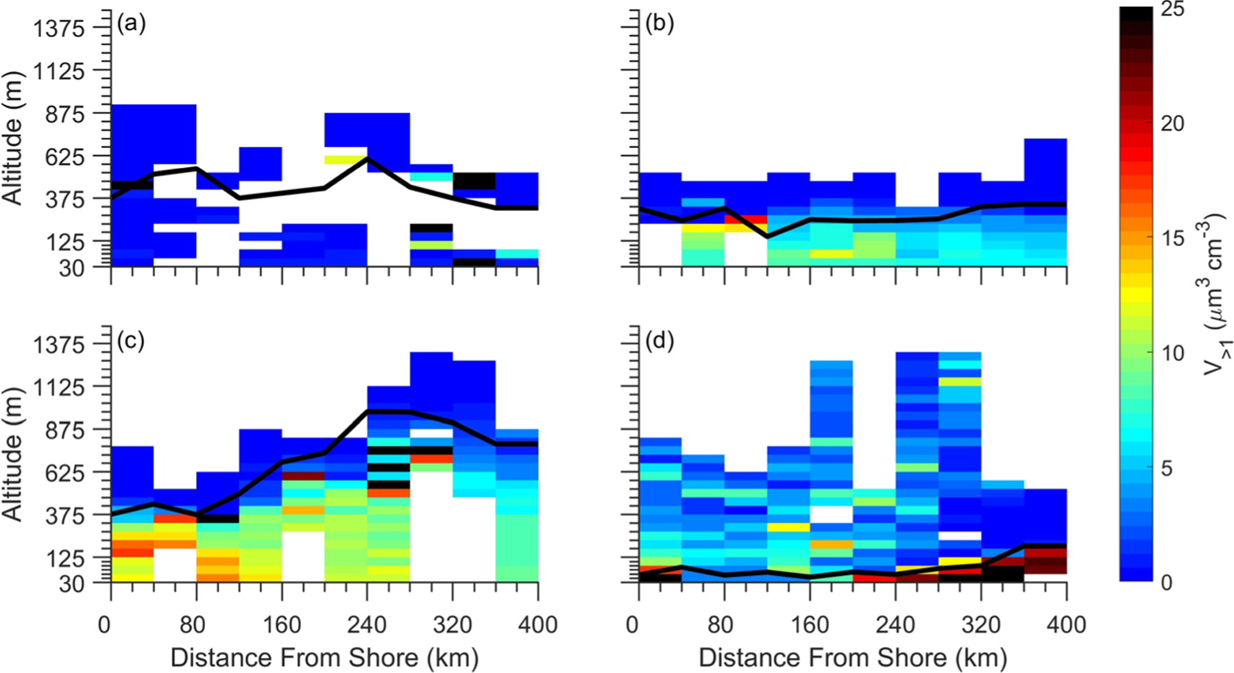
Same as Figure 4 except cells are colored by V_>1 concentration.

The N_>1 and V_>1 concentrations of Regime 2 (RF06) decreased with increasing distance from shore while remaining relatively constant from the near surface to just below the MBL cap. N_>1 and V_>1 concentrations of this regime ranged from ~1.5 to ~4 cm⁻³ and from ~6 to ~12 μm³ cm⁻³, respectively. Similar to Regime 2, the N_>1 and V_>1 concentrations of Regime 3 (RF08) decreased with increasing distance from shore. These concentrations ranged from ~1 to ~3 cm⁻³ and from ~10 to ~13 μm³ cm⁻³, respectively. Although the MBL depth of Regime 3 increased greatly (from ~375 to ~900 m) with increasing distance from shore, the N_>1 and V_>1 concentrations remained relatively constant from the near surface until just below the MBL cap at all distances within the study region.

The N_>1 and V_>1 concentrations observed during Regime 4 (RF10) were relatively constant from the near surface until just below the MBL cap. The N_>1 and V_>1 concentrations of this regime were unique in that they increased with offshore distance. These concentrations ranged from ~1.5 to ~4.5 cm⁻³ and from ~5 to ~25 μm³ cm⁻³, respectively.

3.4. Factors Related to Near Surface SM-SSA

3.4.1. Scatterplots

As demonstrated in the previous sections, different synoptic and meteorological regimes correspond to distinct N_>1 and V_>1 concentration ranges and spatial trends. The following sections aim to examine the relations between near surface N_>1 and V_>1 concentrations and a variety of MBL properties (i.e., wind speed, wind direction, T_amb, SST, TKE, RH, MBL depth, and r_cb). Note that cycle-averaged r_cb values are used hereafter rather than those for ${\overline{\text{r}}}_{\text{cb}}$ to capture effects of wet scavenging for each cycle. Figures 6 and 7 illustrate scatterplot relationships between the near surface N_>1 and V_>1 concentrations, respectively, and MBL properties for all 147 cycles of MONARC. The relationships between these concentrations and the MBL parameters were highly dynamic and varied depending on regime. Consequently, none of cumulative scatterplots had a best fit line that was statistically significant with a p value below 0.05. The corresponding correlation coefficients of each panel are provided in Table S1, with R values ranging from −0.36 to 0.21. The strongest relationships (regardless of sign) for both N_>1 and V_>1 were with r_cb (R = −0.36 and −0.32, respectively). The lack of notable trends discernable from these scatterplots suggests that there are no well-defined relations, especially of a linear nature. Consequently, there may be many factors that govern N_>1 and V_>1 concentrations such as the previous history of sampled air masses that may outweigh influence from local conditions.

Figure 6.

Scatterplots between cycle-averaged values of near surface N_>1 concentration versus several other cycle-averaged MBL conditions.

Figure 7.

Same as Figure 6 but for near surface V_>1 concentration on y-axis.

3.4.2. Machine Learning Analysis

In response to how the previous section showed that scatterplots cannot adequately capture relationships between SM-SSA and MBL properties, assuming that they exist in the data set, here we employ a different approach (i.e., MLR) to determine the best predictors of near surface N_>1 and V_>1 concentrations (Figures 8–12). The first step for MLR analysis was to choose a model among the nine categories of MLR models (e.g., MVLR, three subtypes of SVM, GBRT, bagged regression tree, and three subtypes of GPR).

Figure 8.

Partial dependency (PD) plots for different MBL parameters used as predictors for near surface N_>1 concentration. The solid-blue line represents the mean and the dashed-yellow and dashed-orange lines signify the mean plus and minus one standard deviation, respectively.

Figure 12.

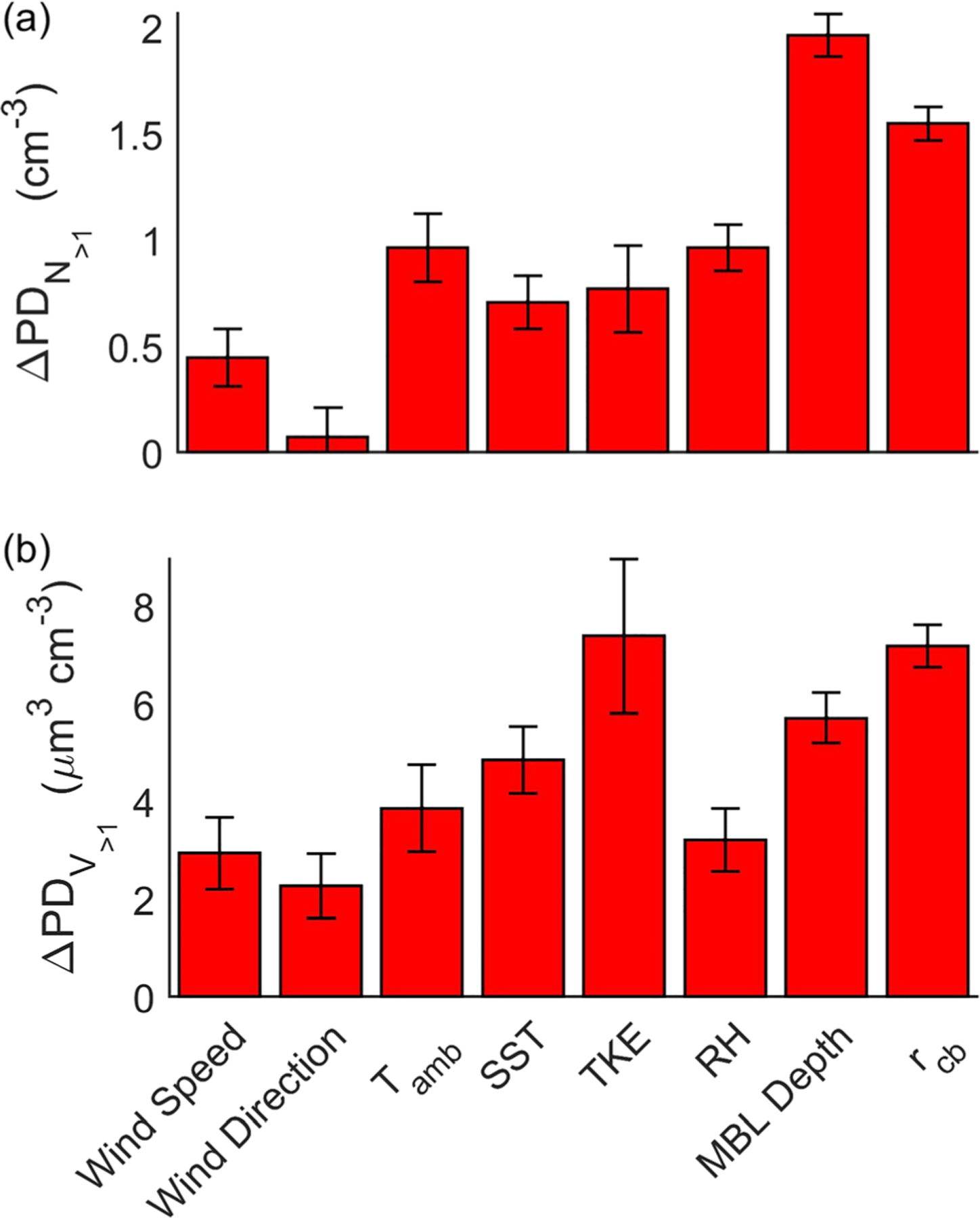
Mean difference in the PD (ΔPD) of different MBL variables used as predictors of near surface (a) N_>1 and (b) V_>1 concentrations. Error bars represent one standard deviation.

The preliminary analysis described in section 2.4 found that cross-validated predictions using the exponential GPR and GBRT models had the lowest MSE values for both N_>1 and V_>1 concentrations. As a next step, the exponential GPR and GBRT models were repetitively trained using random sampling with cross-validation, OOB testing, and grid-search hyperparameter optimization. Table S2 summarizes statistics resulting from OOB testing of the training of the GPR and GBRT models for predicting both N_>1 and V_>1 with the same variables shown in the scatterplots (Figures 6 and 7). Table S2 also shows the R² resulting from MVLR analysis as a base comparison with the more complex MLR models. The exponential GPR models for N_>1 and V have average R² >1 values between 0.74 and 0.76, maximum R² values of 0.91, and minimum R² values between 0.41 and 0.54. The GBRT and MVLR models have lower average R² values for predicting both N_>1 and V_>1 concentrations. The average R² values resulting from GBRT models for predicting N_>1 and V_>1 concentrations were 0.71 and 0.60, respectively, while those resulting from MVLR were 0.15 and 0.13, respectively. Given the robustness of the exponential GPR models as compared to the GBRT and MVLR models, hereafter the discussion centers around the GPR results with regard to relationships between near surface SM-SSA concentrations and other MBL parameters. Note that the analysis is based on local MBL parameters and does not incorporate aspects associated with the air mass history, which could certainly be influential and were previously involved with the regime analysis of sections 3.1–3.3 and 3.4.1.

Partial dependency (PD) plots demonstrate how manipulation of one predictor (i.e., wind speed, wind direction, T_amb, SST, TKE, RH, MBL depth, or r_cb), while holding the other predictors constant in value, changes the response variable (N_>1 and V_>1) within the model (Figures 8 and 9). With the exception of the last two predictors, all are near surface values. Increasing values of PD_N>1 and PD_V>1 indicate that the corresponding change on the x-axis for the value of the specific parameter is conducive to higher concentration values.

Figure 9.

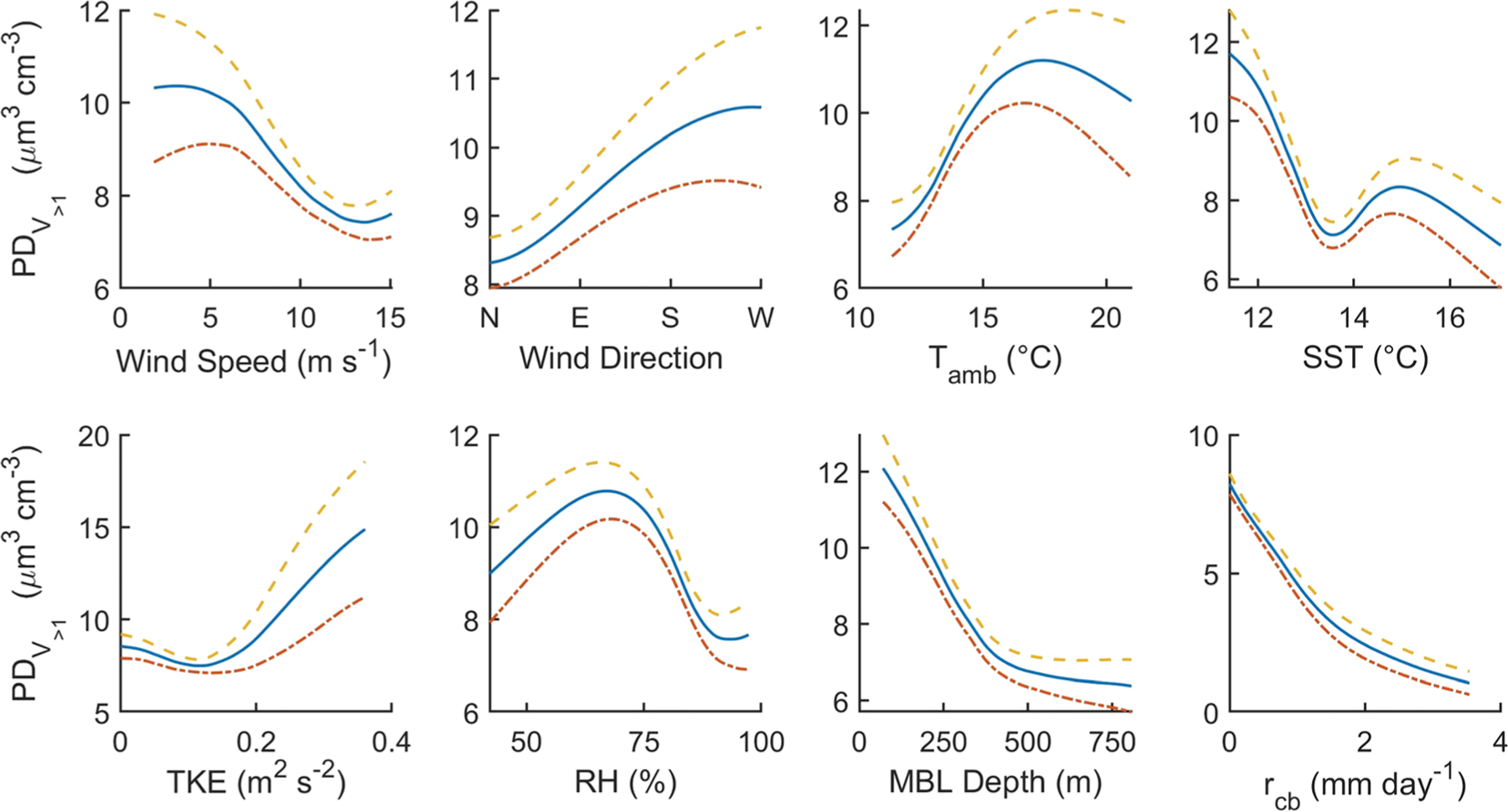
Same as Figure 8 but for near surface V_>1 concentration.

From these PD plots a variety of relationships were noted to be worthy of discussion. Near surface wind speed, which has long been used as the primary driver of SM-SSA emissions (Lewis & Schwartz, 2004; Monahan & Muircheartaigh, 1980), exhibits varying signs in its relationship with N_>1 below (positive) and above 5 m s⁻¹ (negative). The relationship between wind speed and V_>1 concentration is inverse for nearly the entire range of wind speeds. Concentrations of N_>1 and V_>1 were generally negatively related to SST with the caveat that the majority of SST data was below 14°C and within a fairly narrow range.

MBL stability primarily influences the vertical distribution of SSA particles. MBL stability is related to the vertical profiles of near surface wind speed, T_amb, and RH; however, it is generally parameterized by the difference between SST and T_amb. Higher (lower) TKE and RH in conjunction with lower (higher) difference between SST and T_amb corresponds to an unstable (stable) MBL (Lewis & Schwartz, 2004; Monahan et al., 1986). An unstable MBL will enhance turbulence and entrainment rate, and a stable MBL will suppress turbulence and entrainment rate. Enhanced turbulence corresponds to increases in the residence time of larger SSA particles in the MBL. The PD plots demonstrate that both N_>1 and V_>1 concentrations are positively related to T_amb from ~11°C to 15°C, above which the relationship becomes either negative (N_>1) or dampens (V_>1). Caution should be used in the interpretation of the trends between T_amb and N_>1 and V_>1 concentrations for values of T_amb above 15°C due to a limited number of sample points (13% of the total data set). The N_>1 and V_>1 concentrations increase over nearly the entire range of TKE values (especially when TKE was above ~0.15 m² s⁻²). N_>1 (V_>1) concentrations increase with respect to RH from 40% to 80% (40% to 65%); however, N_>1 (V_>1) concentration decreases after RH is greater than 80% (65%). Only 10% of the RH data were below 70%, and interpretation of trends below this range should be viewed with caution.

Higher r_cb values correspond to lower N_>1 and V_>1 concentrations, leveling off above 2 mm day⁻¹ at ~0.50 cm⁻³ and ~1.4 μm³ cm⁻³, respectively. The presence of drizzle within the MBL is known to influence SSA particle lifetime due to wet scavenging (Hoppel et al., 2002) and is usually parameterized by statistical methods within transport models (e.g., Dana & Hales, 1976; MacDonald et al., 2018).

The PD plots show a strong relationship between increasing (decreasing) MBL thickness and decreasing (increasing) N_>1 and V_>1 concentrations, which is presumably because there is a larger (smaller) volume for mixing. This work agrees with previous work by demonstrating an inverse relationship between MBL depth and N_>1 and V_>1 concentrations (Lewis & Schwartz, 2004).

Figures 10 and 11 show surface PD plots for N_>1 and V_>1 concentrations, highlighting the 28 possible combinations in which the response variable can change given the manipulation of two of the six predictors. A few selected results from these surface PD plots are noteworthy and also help reinforce findings already presented from the scatterplots and MLR results in Figures 8 and 9. The surface PD plots demonstrate that maximal N_>1 and V_>1 concentrations will be present with MBL depths below 400 m and r below 1 mm day⁻¹ cb. The plots illustrate well that TKE has a more pronounced impact on V_>1 versus N_>1 when other conditions are held fixed. Finally, the impacts of RH on N_>1 and V_>1 are complex with positive relationships for many panels up to some value (~80% and ~65%, respectively), above which there is a negative relationship. This builds off earlier results with a plausible physical explanation being that at sufficiently high RHs, SM-SSA particles are more swollen and thus evaporate more slowly and have a higher probability of falling back into the water.

Figure 10.

Surface PD plots for 28 unique pairs of MBL parameters used as predictors for near surface N_>1 concentration. Cells are colored by PD of N_>1 concentration.

Figure 11.

Same as Figure 10 but for near surface V_>1 concentration.

Predictor importance (ΔPD) is defined as the difference between the maximum and minimum values of the response associated with the PD analysis of each predictor (Figure 12). The order of importance (in descending order) for predicting N_>1 concentration is MBL depth, r_cb, RH, T_amb, TKE, SST, wind speed, and wind direction. The order of importance for predicting V_>1 concentration is TKE, r_cb, MBL depth, SST, T_amb, RH, wind speed, and wind direction. These importance rankings clearly demonstrate that local wind speed has only a small role in influencing near surface N_>1 and V_>1 concentrations, and this is likely owing to the fact that the air mass history and the winds associated with that history are more influential in driving the MBL SM-SSA concentrations. The results show that MBL depth is more important for predicting N_>1 as compared to V_>1 concentration and drizzle is similarly very influential for both N_>1 and V_>1 concentrations. The results of Figure 12 also confirm earlier results that TKE has a stronger relationship with V_>1 as compared to N_>1.

4. Conclusions

This study examines flight data from the 2019 MONARC campaign, which featured 14 nearly identical flight patterns off the California coast at the same time on different days. The presented analyses take advantage of a statistical approach to airborne data collection in conjunction with MLR techniques with the goal of addressing the nature and character of SM-SSA particles in the MBL over the northeastern Pacific Ocean. The primary results of this study are as follows in order of the questions laid out at the end of section 1:

1. Four MBL regimes were identified during MONARC differing in cloud fraction, air mass source origin, and meteorological and synoptic features. N_>1 and V concentrations (0.8 ± 0.4 cm⁻³ >1 and 3.5 ± 6.5 μm³ cm⁻³, respectively) were lowest in the regime with the highest drizzle rates. The regime with thin MBL depths and negligible drizzle rates coincided with the highest N_>1 concentrations(2.8 ± 0.9 cm⁻³). The highest V_>1 concentrations (12.3 ± 5.7 μm³ cm⁻³), volumetric median diameter(2.7 ± 0.4 μm), and count median diameter (2.4 ± 0.2 μm) coincided with a regime characterized by cloud-free conditions and the highest MBL turbulence and vertical mixing.

2. Vertical SM-SSA profiles are sensitive to MBL depth and r_cb. Profiles of N_>1 and V_>1 as a function of offshore distance either showed a decrease, increase, or no change depending on the MBL regime.

3. Near surface RH (T_amb) were generally negatively (positively) related with both N_>1 and V_>1; however, at some lower RH (higher T_amb) values this relationship was positive (negative). Increases in either MBL depth or r_cb were related to reductions in both N_>1 and V_>1 concentrations. These relationships are likely due to dilution (increased MBL depth) and reduced aerosol lifetime (increased r_cb). Both N_>1 and V_>1 concentrations tended to be positively related to turbulence (i.e., near surface TKE in this study).Based on MLR analysis, MBL depth was found to be the most influential for N_>1, with higher depths corresponding to lower N_>1. TKE was the most important for V_>1, with the two being positively related. Drizzle rate was the second most important predictor (and negatively related) for both N_>1 and V_>1.

4. Of the nine categories of MLR models used to predict near surface N_>1 and V_>1 concentrations, the exponential GPR and GBRT model categories showed higher accuracy than the others without OOB testing or hyperparameter tuning. After OOB training of the exponential GPR and GBRT models using 100 random samples, the set of exponential GPR models had higher average R² values than the set of GBRT models. Based on the apparent robustness of the exponential GPR model, this study presents one set of exponential GPR models for predicting near surface N_>1 and another set of exponential GPR models for predicting near surface V_>1 concentrations.

These results exemplify the utility of data collected with repetitive flight patterns over multiple weeks to analyze relationships between aerosols and MBL conditions. While results from this study are not necessarily similar to what would be found in other regions, the methods developed here can be applied to similar data sets from different regions. The MBL regimes and predictive models can also be utilized by future investigators to compare against other models and near surface measurements.

Figure 4.

Two-dimensional horizontal profile of total N_>1 concentration with respect to distance from the shore for (a) RF03 (Regime 1), (b) RF06 (Regime 2), (c) RF08 (Regime 3), and (d) RF10 (Regime 4). The top of the MBL is indicated with a black line. Cells are colored by N_>1 concentration. Blank cells indicate that the aircraft did not fly in that pixel.

Key Points:

• Vertical and horizontal profiles of supermicron sea salt aerosol concentrations are related to synoptic conditions and air mass history

• Marine boundary layer depth (turbulent kinetic energy) is the best predictor for supermicron sea salt aerosol number (volume) concentration

• Drizzle rate is the second most influential parameter for both supermicron sea salt aerosol number and volume concentration

References

- Andreae MO, & Rosenfeld D (2008). Aerosol–cloud–precipitation interactions. Part 1. The nature and sources of cloud-active aerosols. Earth-Science Reviews, 89, 13–41. 10.1016/j.earscirev.2008.03.001 [DOI] [Google Scholar]
- Andreas EL (1992). Sea spray and the turbulent air-sea heat fluxes. Journal of Geophysical Research, 97(C7), 11,429–11,441. 10.1029/92jc00876 [DOI] [Google Scholar]
- Andreas EL (1995). The temperature of evaporating sea spray droplets. Journal of the Atmospheric Sciences, 52(7), 852–862. [DOI] [Google Scholar]
- Andreas EL (1998). A new sea spray generation function for wind speeds up to 32 m s−1. Journal of Physical Oceanography, 28(11), 2175–2184. [DOI] [Google Scholar]
- Barthel S, Tegen I, & Wolke R (2019). Do new sea spray aerosol source functions improve the results of a regional aerosol model? Atmospheric Environment, 198, 265–278. 10.1016/j.atmosenv.2018.10.016 [DOI] [Google Scholar]
- Beard KV, & Ochs HT (1993). Warm-rain initiation: An overview of microphysical mechanisms. Journal of Applied Meteorology, 32(4), 608–625. [DOI] [Google Scholar]
- Boyce SG (1954). The salt spray community. Ecological Monographs, 24(1), 29–67. 10.2307/1943510 [DOI] [Google Scholar]
- Braun RA, Dadashazar H, MacDonald AB, Aldhaif AM, Maudlin LC, Crosbie E, et al. (2017). Impact of wildfire emissions on chloride and bromide depletion in marine aerosol particles. Environmental Science & Technology, 51, 9013–9021. 10.1021/acs.est.7b02039 [DOI] [PubMed] [Google Scholar]
- Cheng WYY, Carrió GG, Cotton WR, & Saleeby SM (2009). Influence of cloud condensation and giant cloud condensation nuclei on the development of precipitating trade wind cumuli in a large eddy simulation. Journal of Geophysical Research, 114, D08201 10.1029/2008jd011011 [DOI] [Google Scholar]
- Christopoulos CD, Garimella S, Zawadowicz MA, Möhler O, & Cziczo DJ (2018). A machine learning approach to aerosol classification for single-particle mass spectrometry. Atmospheric Measurement Techniques, 11, 5687–5699. 10.5194/amt-11-5687-2018 [DOI] [Google Scholar]
- Collins DR, Johnsson HH, Seinfeld JH, Flagan RC, Gassó S, Hegg DA, et al. (2000). In situ aerosol-size distributions and clear-column radiative closure during ACE-2. Tellus Series B: Chemical and Physical Meteorology, 52, 498–525. 10.3402/tellusb.v52i2.16175 [DOI] [Google Scholar]
- Crosbie E, Brown MD, Shook M, Ziemba L, Moore RH, Shingler T, et al. (2018). Development and characterization of a high-efficiency, aircraft-based axial cyclone cloud water collector. Atmospheric Measurement Techniques, 11, 5025–5048. 10.5194/amt-11-5025-2018 [DOI] [PMC free article] [PubMed] [Google Scholar]
- Dadashazar H, Wang Z, Crosbie E, Brunke M, Zeng X, Jonsson H, et al. (2017). Relationships between giant sea salt particles and clouds inferred from aircraft physicochemical data. Journal of Geophysical Research: Atmospheres, 122, 3421–3434. 10.1002/2016jd026019 [DOI] [Google Scholar]
- Dagan G, Koren I, & Altaratz O (2015). Aerosol effects on the timing of warm rain processes. Geophysical Research Letters, 42,4590–4598. 10.1002/2015gl063839 [DOI] [Google Scholar]
- Dana MT, & Hales JM (1976). Statistical aspects of the washout of polydisperse aerosols. Atmospheric Environment (1967), 10(1), 45–50. 10.1016/0004-6981(76)90258-4 [DOI] [Google Scholar]
- Dong X, Schwantes AC, Xi B, & Wu P (2015). Investigation of the marine boundary layer cloud and CCN properties under coupled and decoupled conditions over the Azores. Journal of Geophysical Research: Atmospheres, 120, 6179–6191. 10.1002/2014jd022939 [DOI] [Google Scholar]
- Fei K, Wu L, & Zeng Q (2019). Aerosol optical depth and burden from large sea salt particles. Journal of Geophysical Research: Atmospheres, 124, 1680–1696. 10.1029/2018jd029814 [DOI] [Google Scholar]
- Feingold G, Cotton WR, Kreidenweis SM, & Davis JT (1999). The impact of giant cloud condensation nuclei on drizzle formation in stratocumulus: Implications for cloud radiative properties. Journal of the Atmospheric Sciences, 56(24), 4100–4117. [DOI] [Google Scholar]
- Feingold G, McComiskey A, Rosenfeld D, & Sorooshian A (2013). On the relationship between cloud contact time and precipitation susceptibility to aerosol. Journal of Geophysical Research: Atmospheres, 118, 10,544–10,554. 10.1002/jgrd.50819 [DOI] [Google Scholar]
- Feng M, Zhang W, Zhu X, Duan B, Zhu M, & Xing D (2018). Multivariate interpolation of wind field based on Gaussian process regression. Atmosphere, 9, 194 10.3390/atmos9050194 [DOI] [Google Scholar]
- Gerber H, Arends BG, & Ackerman AS (1994). New microphysics sensor for aircraft use. Atmospheric Research, 31(4), 235–252. 10.1016/0169-8095(94)90001-9 [DOI] [Google Scholar]
- Graedel TE, & Keene WC (1995). Tropospheric budget of reactive chlorine. Global Biogeochem Cycles, 9(1), 47–77. 10.1029/94gb03103 [DOI] [Google Scholar]
- Hanley KE, Belcher SE, & Sullivan PP (2010). A global climatology of wind–wave interaction. Journal of Physical Oceanography, 40,1263–1282. 10.1175/2010jpo4377.1 [DOI] [Google Scholar]
- Haskins JD, Lee BH, Lopez-Hilifiker FD, Peng Q, Jaeglé L, Reeves JM, et al. (2019). Observational constraints on the formation of Cl2 from the reactive uptake of ClNO2 on aerosols in the polluted marine boundary layer. Journal of Geophysical Research: Atmospheres, 124, 8851–8869. 10.1029/2019jd030627 [DOI] [Google Scholar]
- Haywood JM, Ramaswamy V, & Soden BJ (1999). Tropospheric aerosol climate forcing in clear-sky satellite observations over the oceans. Science, 283(5406), 1299–1303. 10.1126/science.283.5406.1299 [DOI] [PubMed] [Google Scholar]
- Hegg DA, and Hobbs PV (1986), Studies of the mechanisms and rates with which nitrogen species are incorporated into cloud water and precipitation, edited, Second Annual Report on Project CAPA-21–80 to the Coordinating Research Council. [Google Scholar]
- Hoppel WA, Frick GM, & Fitzgerald JW (2002). Surface source function for sea-salt aerosol and aerosol dry deposition to the ocean surface. Journal of Geophysical Research, 107(D19), 4382 10.1029/2001jd002014 [DOI] [Google Scholar]
- Hughes M, Kodros JK, Pierce JR, West M, & Riemer N (2018). Machine learning to predict the global distribution of aerosol mixing state metrics. Atmosphere, 9, 15 10.3390/atmos9010015 [DOI] [Google Scholar]
- Jaeglé L, Quinn PK, Bates TS, Alexander B, & Lin JT (2011). Global distribution of sea salt aerosols: New constraints from in situ and remote sensing observations. Atmospheric Chemistry and Physics, 11, 3137–3157. 10.5194/acp-11-3137-2011 [DOI] [Google Scholar]
- James G, Witten D, Hastie T, & Tibshirani R (2013). An introduction to statistical learning: With applications in R, (1st ed.p. 426). New York: Springer Publishing Company, Inc. 10.1007/978-1-4614-7138-7 [DOI] [Google Scholar]
- Johnson DB (1982). The role of giant and ultragiant aerosol particles in warm rain initiation. Journal of the Atmospheric Sciences, 39(2), 448–460. [DOI] [Google Scholar]
- Jung E, Albrecht BA, Jonsson HH, Chen YC, Seinfeld JH, Sorooshian A, et al. (2015). Precipitation effects of giant cloud condensation nuclei artificially introduced into stratocumulus clouds. Atmospheric Chemistry and Physics, 15, 5645–5658. 10.5194/acp-15-5645-2015 [DOI] [Google Scholar]
- Keene WC, Long MS, Reid JS, Frossard AA, Kieber DJ, Maben JR, et al. (2017). Factors that modulate properties of primary marine aerosol generated from ambient seawater on ships at sea. Journal of Geophysical Research: Atmospheres, 122, 11,961–11,990. 10.1002/2017jd026872 [DOI] [Google Scholar]
- Keene WC, Maring H, Maben JR, Kieber DJ, Pszenny AAP, Dahl EE, et al. (2007). Chemical and physical characteristics of nascent aerosols produced by bursting bubbles at a model air-sea interface. Journal of Geophysical Research, 112, D21202 10.1029/2007jd008464 [DOI] [Google Scholar]
- Kelly JT, Chuang CC, & Wexler AS (2007). Influence of dust composition on cloud droplet formation. Atmospheric Environment, 41, 2904–2916. 10.1016/j.atmosenv.2006.12.008 [DOI] [Google Scholar]
- Kogan YL, Mechem DB, & Choi K (2012). Effects of sea-salt aerosols on precipitation in simulations of shallow cumulus. Journal of the Atmospheric Sciences, 69, 463–483. 10.1175/jas-d-11-031.1 [DOI] [Google Scholar]
- L’Ecuyer TS, Berg W, Haynes J, Lebsock M, & Takemura T (2009). Global observations of aerosol impacts on precipitation occur-rence in warm maritime clouds. Journal of Geophysical Research, 114, D09211 10.1029/2008jd011273 [DOI] [Google Scholar]
- Lenain L, & Melville WK (2017). Evidence of sea-state dependence of aerosol concentration in the marine atmospheric boundary layer. Journal of Physical Oceanography, 47, 69–84. 10.1175/jpo-d-16-0058.1 [DOI] [Google Scholar]
- Lewis ER, & Schwartz SE (2004). Sea salt aerosol production: Mechanisms, methods, measurements, and models. Washington, DC: American Geophysical Union. [Google Scholar]
- MacDonald AB, Dadashazar H, Chuang PY, Crosbie E, Wang H, Wang Z, et al. (2018). Characteristic vertical profiles of cloud water composition in marine stratocumulus clouds and relationships with precipitation. Journal of Geophysical Research: Atmospheres, 123, 3704–3723. 10.1002/2017jd027900 [DOI] [PMC free article] [PubMed] [Google Scholar]
- Marsden NA, Ullrich R, Möhler O, Eriksen Hammer S, Kandler K, Cui Z, et al. (2019). Mineralogy and mixing state of north African mineral dust by online single-particle mass spectrometry. Atmospheric Chemistry and Physics, 19, 2259–2281. 10.5194/acp-19-2259-2019 [DOI] [Google Scholar]
- Mårtensson EM, Nilsson ED, de Leeuw G, Cohen LH, & Hansson H-C (2003). Laboratory simulations and parameterization of the primary marine aerosol production. Journal of Geophysical Research, 108, 4297 10.1029/2002jd002263 [DOI] [Google Scholar]
- Maudlin LC, Wang Z, Jonsson HH, & Sorooshian A (2015). Impact of wildfires on size-resolved aerosol composition at a coastal California site. Atmospheric Environment, 119, 59–68. 10.1016/j.atmosenv.2015.08.039 [DOI] [Google Scholar]
- Monahan EC (1968). Sea spray as a function of low elevation wind speed. Journal of Geophysical Research, 73(4), 1127–1137. 10.1029/JB073i004p01127 [DOI] [Google Scholar]
- Monahan EC, & Muircheartaigh I (1980). Optimal power-law description of oceanic whitecap coverage dependence on wind speed. Journal of Physical Oceanography, 10(12), 2094–2099. [DOI] [Google Scholar]
- Monahan EC, Spiel DE, & Davidson KL (1986). A model of marine aerosol generation via whitecaps and wave disruption In Monahan EC, & Niocaill GM (Eds.), Oceanic whitecaps: And their role in air-sea exchange processes, (pp. 167–174). Dordrecht: Springer Netherlands; 10.1007/978-94-009-4668-2_16 [DOI] [Google Scholar]
- Murphy DM, Anderson JR, Quinn PK, McInnes LM, Brechtel FJ, Kreidenweis SM, et al. (1998). Influence of sea-salt on aerosol radiative properties in the Southern Ocean marine boundary layer. Nature, 392(6671), 62–65. 10.1038/32138 [DOI] [Google Scholar]
- Murphy DM, Froyd KD, Bian H, Brock CA, Dibb JE, DiGangi JP, et al. (2019). The distribution of sea-salt aerosol in the global troposphere. Atmospheric Chemistry and Physics, 19(6), 4093–4104. 10.5194/acp-19-4093-2019 [DOI] [Google Scholar]
- Partanen AI, Dunne EM, Bergman T, Laakso A, Kokkola H, Ovadnevaite J, et al. (2014). Global modelling of direct and indirect effects of sea spray aerosol using a source function encapsulating wave state. Atmospheric Chemistry and Physics, 14, 11,731–11,752. 10.5194/acp-14-11731-2014 [DOI] [Google Scholar]
- Prabhakar G, Ervens B, Wang Z, Maudlin LC, Coggon MM, Jonsson HH, et al. (2014). Sources of nitrate in stratocumulus cloud water: Airborne measurements during the 2011 E-PEACE and 2013 NiCE studies. Atmospheric Environment, 97, 166–173. 10.1016/j.atmosenv.2014.08.019 [DOI] [Google Scholar]
- Radke LF, Hegg DA, Lyons JH, Brock CAH, Peter V, Weiss RE, & Rasmussen RA (1988). Airborne measurements on smokes from biomass burning In Hobbs PV, & McCormick MP (Eds.), Aerosols and climate, (pp. 411–422). Hampton, VA: A. Deepak Publishing Co. [Google Scholar]
- Reid JS, Brooks B, Crahan KK, Hegg DA, Eck TF, O’Neill N, et al. (2006). Reconciliation of coarse mode sea-salt aerosol particle size measurements and parameterizations at a subtropical ocean receptor site. Journal of Geophysical Research, 111, D02202 10.1029/2005jd006200 [DOI] [Google Scholar]
- Reid JS, Jonsson HH, Smith MH, & Smirnov A (2001). Evolution of the vertical profile and flux of large sea-salt particles in a coastal zone. Journal of Geophysical Research, 106(D11), 12,039–12,053. 10.1029/2000jd900848 [DOI] [Google Scholar]
- Salter ME, Zieger P, Acosta Navarro JC, Grythe H, Kirkevåg A, Rosati B, et al. (2015). An empirically derived inorganic sea spray source function incorporating sea surface temperature. Atmospheric Chemistry and Physics, 15, 11047–11066. 10.5194/acp-15-11047-2015 [DOI] [Google Scholar]
- Skartveit A (1982). Wet scavenging of sea-salts and acid compounds in a rainy, coastal area. Atmospheric Environment (1967), 16(11), 2715–2724. 10.1016/0004-6981(82)90356-0 [DOI] [Google Scholar]
- Sofiev M, Soares J, Prank M, de Leeuw G, & Kukkonen J (2011). A regional-to-global model of emission and transport of sea salt particles in the atmosphere. Journal of Geophysical Research, 116, D021302 10.1029/2010jd014713 [DOI] [Google Scholar]
- Sorooshian A, MacDonald AB, Dadashazar H, Bates KH, Coggon MM, Craven JS, et al. (2018). A multi-year data set on aerosol-cloud-precipitation-meteorology interactions for marine stratocumulus clouds. Scientific Data, 5, 180026 10.1038/sdata.2018.26 [DOI] [PMC free article] [PubMed] [Google Scholar]
- Sorooshian A, Prabhakar G, Jonsson H, Woods RK, Flagan RC, & Seinfeld JH (2015). On the presence of giant particles downwind of ships in the marine boundary layer. Geophysical Research Letters, 42, 2024–2030. 10.1002/2015gl063179 [DOI] [Google Scholar]
- Sorooshian A, et al. (2017), A multi-year data set on aerosol-cloud-precipitation-meteorology interactions for marine stratocumulus clouds, doi: 10.6084/m9.figshare.5099983.v10 [DOI] [PMC free article] [PubMed] [Google Scholar]
- Stein AF, Draxler RR, Rolph GD, Stunder BJB, Cohen MD, & Ngan F (2015). NOAA’s HYSPLIT atmospheric transport and dispersion modeling system. Bulletin of the American Meteorological Society, 96(12), 2059–2077. 10.1175/bams-d-14-00110.1 [DOI] [Google Scholar]
- Stramska M, & Petelski T (2003). Observations of oceanic whitecaps in the north polar waters of the Atlantic. Journal of Geophysical Research, 108(C3), 3086 10.1029/2002jc001321 [DOI] [Google Scholar]
- Takemura T, Okamoto H, Maruyama Y, Numaguti A, Higurashi A, & Nakajima T (2000). Global three-dimensional simulation of aerosol optical thickness distribution of various origins. Journal of Geophysical Research, 105(D14), 17,853–17,873. 10.1029/2000jd900265 [DOI] [Google Scholar]
- Teller A, & Levin Z (2006). The effects of aerosols on precipitation and dimensions of subtropical clouds: A sensitivity study using a numerical cloud model. Atmospheric Chemistry and Physics, 6, 67–80. 10.5194/acp-6-67-2006 [DOI] [Google Scholar]
- Textor C, Schulz M, Guibert S, Kinne S, Balkanski Y, Bauer S, et al. (2006). Analysis and quantification of the diversities of aerosol life cycles within AeroCom. Atmospheric Chemistry and Physics, 6, 1777–1813. 10.5194/acp-6-1777-2006 [DOI] [Google Scholar]
- Veron F (2015). Ocean spray. Annual Review of Fluid Mechanics, 47, 507–538. 10.1146/annurev-fluid-010814-014651 [DOI] [Google Scholar]
- Veron F, Hopkins C, Harrison E, & Mueller J (2012). Sea spray spume droplet production in high wind speeds. Geophysical Research Letters, 39, L16602 10.1029/2012gl052603 [DOI] [Google Scholar]
- Wang Z, Mora Ramirez M, Dadashazar H, MacDonald AB, Crosbie E, Bates KH, et al. (2016). Contrasting cloud composition between coupled and decoupled marine boundary layer clouds. Journal of Geophysical Research: Atmospheres, 121, 11,679–11,691. 10.1002/2016jd025695 [DOI] [Google Scholar]
- Wang Z, Sorooshian A, Prabhakar G, Coggon MM, & Jonsson HH (2014). Impact of emissions from shipping, land, and the ocean on stratocumulus cloud water elemental composition during the 2011 E-PEACE field campaign. Atmospheric Environment, 89, 570–580. 10.1016/j.atmosenv.2014.01.020 [DOI] [Google Scholar]
- Woodcock AH (1952). Atmospheric salt particles and raindrops. Journal of Meteorology, 9(3), 200–212. [DOI] [Google Scholar]
- Wu J (1975). Wind-induced drift currents. Journal of Fluid Mechanics, 68(01), 49–70. 10.1017/S0022112075000687 [DOI] [Google Scholar]
- Zábori J, Matisāns M, Krejci R, Nilsson ED, & Ström J (2012). Artificial primary marine aerosol production: A laboratory study with varying water temperature, salinity, and succinic acid concentration. Atmospheric Chemistry and Physics, 12, 10,709–10,724. 10.5194/acp-12-10709-2012 [DOI] [Google Scholar]
- Zhao D, & Toba Y (2001). Dependence of whitecap coverage on wind and wind-wave properties. Journal of Oceanography, 57(5), 603–616. 10.1023/a:1021215904955 [DOI] [Google Scholar]
- Zhou Y, Varner RK, Russo RS, Wingenter OW, Haase KB, Talbot R, & Sive BC (2005). Coastal water source of short-lived halocarbons in New England. Journal of Geophysical Research, 110, D21302 10.1029/2004jd005603 [DOI] [Google Scholar]
- Zieger P, Väisänen O, Corbin JC, Partridge DG, Bastelberger S, Mousavi-Fard M, et al. (2017). Revising the hygroscopicity of inorganic sea salt particles. Nature Communications, 8, 15883 10.1038/ncomms15883 [DOI] [PMC free article] [PubMed] [Google Scholar]
Associated Data
This section collects any data citations, data availability statements, or supplementary materials included in this article.