

Abstract
In an effort to better represent aerosol transport in mesoscale and global-scale models, large eddy simulations (LES) from the National Center for Atmospheric Research (NCAR) Turbulence with Particles (NTLP) code are used to develop a Markov chain random walk model that predicts aerosol particle profiles in a cloud-free marine atmospheric boundary layer (MABL). The evolution of vertical concentration profiles are simulated for a range of aerosol particle sizes and in a neutral and an unstable boundary layer. For the neutral boundary layer we find, based on the LES statistics and a specific model time step, that there exist significant correlation for particle positions, meaning that particles near the bottom of the boundary are more likely to remain near the bottom of the boundary layer than being abruptly transported to the top, and vice versa. For the unstable boundary layer, a similar time interval exhibits a weaker tendency for an aerosol particle to remain close to its current location compared to the neutral case due to the strong nonlocal convective motions. In the limit of a large time interval, particles have been mixed throughout the MABL and virtually no temporal correlation exists. We leverage this information to parameterize a Markov chain random walk model that accurately predicts the evolution of vertical concentration profiles. The new methodology has significant potential to be applied at the subgrid level for coarser-scale weather and climate models, the utility of which is shown by comparison to airborne field data and global aerosol models.
1. Introduction
At the ocean surface, the combination of winds and breaking waves generate sea spray aerosol droplets that are transported throughout the marine atmospheric boundary layer (MABL) (Andreas, 1998; de Leeuw et al., 2000; Veron, 2015). Suspended in the atmosphere, sea spray aerosol particles can act as cloud condensation nuclei (Clarke et al., 2006; Ghan et al., 1998; Lewis & Schwartz, 2004), influence the propagation of electromagnetic radiation (Gerber, 1991; Stolaki et al., 2015), and interact with geochemical cycles of reactant species (Erickson et al., 1999). The impact on these processes depends on the aerosol number concentration, mass loading, chemical composition, and sea spray droplet size, which spans a wide distribution (Quinn et al., 2015; Reid et al., 2008). To address these influences, observational and model-based studies have investigated the vertical distribution of sea spray aerosol particles in the atmosphere (Bian et al., 2019; Liang et al., 2016; Reid et al., 2001).
To study the effect of turbulence on aerosol particle transport processes, high fidelity numerical simulations of the MABL can be used. In particular, large eddy simulations (LESs) have been used to understand the dynamics of boundary layers (Moeng, 1984), characterize their statistical turbulence properties (Deardorff, 1972), and investigate plume dispersion (Lamb, 1978; Wyngaard & Brost, 1984). Lagrangian models have also been considered for particle transport and dispersion in open channel turbulent boundary layers (Shi & Yu, 2015). Upscaling the governing physical processes with bulk parameters is of interest due to the large computational cost associated with explicitly resolving the wide distribution of length and timescales in the MABL. In environmental fluid flows, the ratio between the largest and smallest length scales of motion can span more than 6 orders of magnitude. To alleviate the cost of attempting to resolve all scales, modelers use coarse-grid resolutions; global aerosol models as well as mesoscale systems have grid lengths between one and hundreds of kilometers (Lynch et al., 2016; Riemer et al., 2003). Consequently, large-scale models then neglect small-scale processes, but it is imperative to provide coarse-scale models with accurate representations of subgrid distributions of aerosol particle concentrations. This representation is particularly important along the sea surface, where aerosol particles are generated and are mostly confined (Blanchard et al., 1984; Toba, 1965).
One approach for parameterizing the turbulent transport of sea spray aerosol particles in the MABL has been through the use of one-dimensional column models (Caffrey et al., 2006; Kind, 1992; Prandtl, 1981; Rouse, 1937). These models attempt to describe vertical concentration profiles that account for gravitational settling as well as net surface emission and have been extended to account for a range of atmospheric stabilities (Chamecki et al., 2007; Freire et al., 2016). These studies rely on Monin-Obukhov similarity theory to predict aerosol concentration profiles in the surface layer; Nissanka et al. (2018) extended this to capture profiles for the full MABL. While Nissanka et al. (2018) (hereafter referred to as N18) provide reasonable predictions in the case of neutral stability, expressing turbulent fluxes in an unstable boundary layer by the gradient diffusion hypothesis (also known as first-order K theory) limits the accuracy of the prediction of vertical concentration profiles (Stull, 1988). As N18 points out, the proposed one-dimensional column model cannot reproduce the uniform concentrations with height, and so a different approach is needed. As motivation to address the limitation of the model presented by N18, we propose one such alternative approach, maintaining both rapid and accurate predictions of aerosol concentrations for varying size and stability. This approach can be served as a parameterization method in global and perhaps mesoscale aerosol models.
To do this, we upscale transport using a correlated random walk method. Random walk frameworks are commonplace, ranging across applications including financial markets (Montero & Masoliver, 2017; Scalas, 2006), electron transport (Nelson, 1999), animal foraging patterns (Giuggioli et al., 2009), and solute transport in hydrogeologic systems (Berkowitz et al., 2006; Le Borgne et al., 2008). Particle trajectories through space and time are modeled as a series of stochastic jumps (i.e., random walk), most commonly sampled as independent and identically distributed. In this study, however, we adopt a correlation-based random walk model that is conceptually similar to that applied in the subsurface hydrology community (Bolster et al., 2014; De Anna et al., 2013; Le Borgne et al., 2008). Here we define correlation as the probability of particle transport from one location over given a model time step given an initial starting location. The key assumption in a correlated random walk model is that a particle’s transport behavior at every model step is dependent on its current state, thus having a one-step memory.
We apply this random walk framework to model the evolution of a constant surface source of aerosol particles in the MABL. Aerosol particle mass is discretized into many point particles that transition through time and space by sampling a probability distribution that governs particle motion. Specifically, we model a particle’s vertical position through time. By considering many particle trajectories, our upscaled framework predicts the vertical transport of aerosol particles through a cloud-free MABL, allowing effective modeling of the temporal evolution of vertical concentration profiles. Similar upscaled transport models in the context of hydrologic systems have displayed computational costs 6 orders of magnitude less than high fidelity simulations (e.g., Sherman et al., 2019), meaning that transport behavior can be faithfully predicted at future times without resolving the turbulent flow field. Though the focus of this study is geared toward sea spray aerosol particles over the open ocean, this modeling strategy can in principle be applied to anthropogenic, dust, or any other kind of particle over various landscapes. In this study, we test the robustness of our method by considering both neutral and unstable boundary layers and for a range of aerosol particle sizes. Although the model is trained on known, idealized LES simulations, the proposed modeling framework here is used as a validation of theory to offer a step toward an accurate, computationally efficient aerosol particle transport model.
2. Numerical Methodology
2.1. LESs
This study uses a modified version of the National Center for Atmospheric Research (NCAR) LES model (Moeng, 1984), which includes Lagrangian particles (referred to as NTLP, NCAR Turbulence with Lagrangian Particles). The Eulerian fields of mass, momentum, and energy are solved from the filtered Navier-Stokes equations under the Boussinesq approximation:
| (1) |
| (2) |
| (3) |
where is the resolved velocity, is the resolved potential temperature, is the resolved pressure, τij is the subgrid stress, f is the Coriolis parameter, and τθi is the subgrid turbulent flux of potential temperature. The Eulerian subgrid-scale turbulent fluxes are parameterized with a prognostic equation that solves for the subgrid-scale turbulent energy, which is then used to define a mixing length. Further subgrid-scale parameterization detail can be found in Deardorff (1980).
We assume the large-scale pressure gradient balances the Coriolis force by imposing a constant geostrophic wind speed, Ug. The flow is driven by this geostrophic wind, in which only one direction is considered (Ug = 10m/s, Vg = 0). The Eulerian representation of the carrier phase is assumed periodic in the horizontal (x and y) directions and resolved on a uniform grid in all Cartesian directions. An inversion layer (zinv) is imposed at the upper half of the domain’s vertical extent, in addition to a radiation condition at the top of the domain (Klemp & Durran, 1983). A pseudospectral discretization is used for spatial gradients in the horizontal directions, whereas a second-order finite difference scheme is used in the vertical direction. Time integration is done with a third-order Runge-Kutta method, and a divergence-free filtered velocity field is enforced via a fractional step method. The lower boundary conditions are prescribed by the rough-wall Monin-Obukhov similarity relations, and the surface is assumed flat with a constant aerodynamic roughness (0.001 m). The base LES model (without Lagrangian point-particles) has been used previously in many studies of the planetary boundary layer (Moeng, 1984; Moeng & Wyngaard, 1988).
Sea spray aerosol particles are represented as Lagrangian point particles, which are assumed smaller than the smallest scales of turbulence (Balachandar & Eaton, 2010). Particle motion follows a Langevin equation:
| (4) |
| (5) |
where the velocity of the particle (vp, i) is dictated by the local resolved fluid velocity (uf, i), which is retrieved at the location of the particle using sixth-order Lagrange interpolation. It is further modulated by the settling velocity τpg, where is the Stokes timescale for a sphere (Brennen, 2005). In Equation 4, ηi is an independent and identically distributed random value from a normal distribution. The subgrid diffusivity K(xp, i) describes the turbulent dispersion of the Lagrangian particle; it is obtained from the LES subgrid eddy diffusivity (for a passive scalar) interpolated to the particle location. Overbars refer to averaging in the horizontal directions. The fourth term, , takes into account vertical transport that is caused by spatial variations in mean diffusivities and conserves mass balance that would otherwise be violated (see Delay et al., 2005, Equation 40, for more details).
For our particular simulation setups, the domain size and number of grid points are held fixed at 1,500 × 1,500 × 850 m (x × y × z) and 128 × 128 × 128, respectively. This grid configuration is similar to other atmospheric boundary layer studies (Sullivan & Patton, 2011; Sullivan et al., 1998). The time step is set to 0.5 s with an initial temperature inversion of 0.50 K/m at approximately 570 m. The use of the strong inversion is to maintain approximate, statistically steady state conditions with minimal boundary layer growth. We consider aerosol particle sizes with diameters of 2, 10, and 50 μm to test the influence of gravitational settling on transport behavior and aerosol particle lifetime.
Two simulations without particles are performed to allow the turbulent flow field to fully develop and reach statistically steady state conditions. The first one corresponds to 3 hr with neutral atmospheric stability, whereas the second run is for 1 hr with unstable stratification. The same geostrophic wind (Ug = 10 m/s) is imposed on both neutral and unstable cases. For the unstable case, a surface heat flux of 0.02 K-m/s is used. In relation to meteorological conditions, this corresponds to an air-sea temperature difference of roughly 1.5 K. Once the flow field fully develops, monodisperse particles are generated randomly along an x-y plane at the first vertical grid point (z = 3.12 m); 100 particles are initialized at each LES time step (200 particles per second). The source flux is denoted as ϕs = 200 s−1. If the Lagrangian particles are transported below the lower surface (xp, 3 ≤ 0), the particle is removed from the simulation, representing dry deposition.
LES, like all models, makes explicit assumptions and is only valid when those assumptions are reasonable. In the LES considered here, the simulated Lagrangian sea spray aerosol particles maintain a constant size, meaning that hygroscopicity and aerosol swell are not considered (Winkler, 1988). The changing atmospheric conditions due to the diurnal cycle have been neglected, as have momentum and energy exchange between the aerosol particles and the air (e.g., neglecting the effects of spray modifying heat and moisture in the surface layer Peng & Richter, 2019). Lastly, the LES assumes a flat surface with a prescribed aerodynamic roughness length, although in the open ocean the moving surface waves may play a substantial role in the transport and fate of sea spray aerosol particles (Richter et al., 2019).
2.2. Markov Chain Random Walk Model
Particle transport behavior simulated in the LES is used to develop the upscaled random walk model. As an initial model formulation, we consider only the vertical transport of aerosol particles, where a full 3-D representation can be developed in future studies. In the Markov chain random walk framework, particles transition through time and space by sampling a probabilistic distribution for spatial and temporal jumps ϕ(x, t). A particle’s trajectory is conceptualized as series of jumps, where each jump has an associated distance and time; this is the basis of a random walk model. Here we fix time, meaning each jump occurs over a constant model time step τ, but the associated travel distance varies. The trajectory can therefore be expressed as ϕ(x, t) = Ψ(x)δ(t − τ). Physically, the sampled travel distance represents the net vertical displacement of a particle over the given lapse time τ.
With this, we can describe particle motion with the Langevin equation
| (6) |
At every model step, particle i travels a vertical displacement ℓ over model time step τ. This vertical displacement at every model step is sampled from a global distribution Ψ(ℓ), in which Ψ(ℓ) is dependent upon the current location of the particle (Ψ(ℓn + 1|ℓn). Hence, since the displacement is sampled from a conditional distribution, particle trajectories are conceptualized as a Markov chain. In this Markov chain random walk framework, particle trajectories are conditionally sampled via a transition matrix (elaborated further below), which gives the probability that a particle transitions from its current height to any other z location in the boundary layer after model time step τ.
Successive model jumps may be spatially independent (or decorrelated), meaning that a particle’s predicted vertical position, given a τ, is independent of its initial position. If independence is assumed, then a randomly sampled location would suffice. Conversely, over shorter model timescales τ, it becomes appropriate to account for this correlation; that is, particles at the bottom (or top) of the boundary layer are more likely to stay at the bottom (or top) of the boundary layer. Again, temporal correlation refers to the probability of particle transport from one location to another over a model time step given a starting location. Therefore, we note that the random walk framework describes the overall model, with temporal correlation via the transition matrix M as a specialized case.
2.2.1. Transition Matrix
To further expand upon the framework of particle displacement, we introduce the transition matrix M. It contains the probabilistic information for any particle jump from any starting location in a fixed time. In the Markov chain model, particles transition through space according to the probabilistic rules of M. As the global distribution Ψ(ℓ) implies a continuous variable, we discretize the atmospheric boundary layer into S height bins, with bins 1 and S representing the lowest and highest vertical positions in the boundary layer, respectively. The matrix M then has size [S, S] and each element in Mi, j is the probability that a particle trajectory after n + 1 model jumps ends in bin j given its initial start bin i at model step n; that is,
| (7) |
By rules of probability, the sum of probabilities of any row in M must be unity. The transition matrix assumes that particle transport behavior can be represented through a one-step memory (the model step time τ), hence being a Markov chain process. Particles sample a distribution for their next location based on its starting bin, and once the particles are displaced (to bin (j)), the same M is used to predict the next model step displacement of particles; M is assumed to be stationary. One of the benefits of this transition matrix approach is that it can model nonlocal behaviors (i.e., particles can jump large distances in the domain and are not just restricted to communicate with adjacent cells). The sensitivity of M is further explored in section 4.4.
In the LES, detailed statistics gathered from a large number of individual Lagrangian particle trajectories are used to construct M. Specifically, we run a steady-state LES simulation over a time τ (Equation 6) and track many (O(106)) particles to estimate each element of M. The particles begin uniformly dispersed throughout the boundary layer height, meaning that each starting bin is weighted equally. A separate LES calculation is performed for each aerosol particle size to construct the size-dependent transition matrices.
The total simulation time required to run the LES consists of the time for the LES to develop statistically steady-state turbulence, and then an additional time τ to compute the transition matrix M as well as the injection distribution ΨI (explained later) of the random walk model. The goal is to only need to run the LES for a time τ, from which the upscaled model can make predictions out to much later times. In this study, the boundary layer is partitioned into 20 bins of equal size; that is, each bin has height of approximately 15 m. With complete information of M and an initial particle location, we can effectively model a particle’s vertical position through time and therefore predict the evolution of vertical aerosol particle concentration profiles.
2.2.2. Boundary Condition: Removal of Particles
Aerosol particles that reach the ocean surface by dry deposition (xp, 3 < 0) in the LES are removed from the simulation. Such behavior must therefore also be faithfully captured within the Markov chain random walk model. To do so, we add an additional bin to M, representing transport to the ocean surface. If a particle transitions to this surface bin, the particle is removed from the system. In the context of stochastic models this is often called transport to a limbo state (Sund et al., 2015; Van Kampen, 1979). Parameterization of this “limbo” bin is consistent with the methods discussed above; that is, in the LES we track the number of particles that transition from height z to the surface after τ, and this is included in the transition matrix M as an additional column. In the results section, the choice of τ is shown to influence the probabilities of dry deposition.
2.2.3. Initial Condition: Particle Injection ΨI(z)
For the MABL system considered here, sea spray aerosol particles are continuously emitted from the ocean surface into the atmospheric boundary layer. This means that under certain conditions, namely, when the number of aerosol particles injected into the atmosphere exceeds the number of aerosol particles depositing onto the ocean surface, the total aerosol particle number will increase through time. We parameterize this behavior in the Markov chain random walk model by adding a distribution of aerosol particles at every model step. This distribution corresponds to the vertical distribution of any new particles generated over the last τ seconds. We first numerically calculate ΨI from LES statistics; ΨI is simply the vertical concentration profile of particles released during a window of time τ. Additionally, we demonstrate that in neutral conditions, ΨI can be parameterized from existing one-dimensional models, potentially removing the need to calculate ΨI from LES. In this study, we assume that the ΨI distribution is stationary for any interval [t, t + τ], though ΨI varies slightly across various intervals for unstable cases. In the LES we add 200 particles per second to the domain, and therefore 200τ for a random walk model time step. Note that the actual injected number is slightly less than 200τ because some particles are emitted and absorbed back into the ocean within the model time step τ; that is, the lifetime of a particle is permitted to be less than τ.
3. Results
Here we briefly summarize the parameterization of the Markov chain random walk model after statistically steady-state turbulence is achieved. Using LES, we find the two upscaled model input parameters: M and ΨI. This is done for each atmospheric condition/particle diameter combination. In this section, we first characterize the neutrally stratified boundary layer and use the LES particle statistics for the comparison and validation of the upscaled model. Afterward, we perform the same procedure for an unstably stratified boundary layer.
3.1. Neutral Boundary Layer
Once aerosol particles are generated at the surface, the vertical transport mechanisms affecting their displacement are the local turbulence and the settling effect of gravity. If the magnitude of settling is less than that of the vertical velocity seen by the Lagrangian particles throughout their lifetime, then they have a high probability of reaching the top of the boundary layer. If particles are too heavy, they have a high likelihood of quickly falling back into the ocean. In the case of neutral boundary layers, the wind shear is solely responsible for the mechanical generation of turbulence. Therefore, characterizing the turbulent kinetic energy (or specifically the vertical velocity variance) is useful in understanding vertical transport of sea spray aerosol particles. Neutral boundary layers as an atmospheric state can be used as a helpful model development testbed and as a proxy for other conditions (Stull, 1988).
3.1.1. Characterization of the Neutral Boundary Layer
For the neutral case, Figure 1 presents snapshots of LES vertical velocity, with horizontal planes at two heights: 100 and 300 m, corresponding to z/zinv = 0.18 and z/zinv = 0.53, where zinv is the boundary layer height. Near the surface, coherent structures of vertical velocities are smaller than near the middle of the boundary layer (300 m), where larger-scale coherent turbulent structures are more visibly apparent. In Figure 1c, the normalized root-mean-square of the vertical velocity exhibits a peak near the surface, in accordance with other studies (Deardorff, 1972). This quantity can be interpreted as a measure of the turbulence intensity experienced by the aerosol particles.
Figure 1.
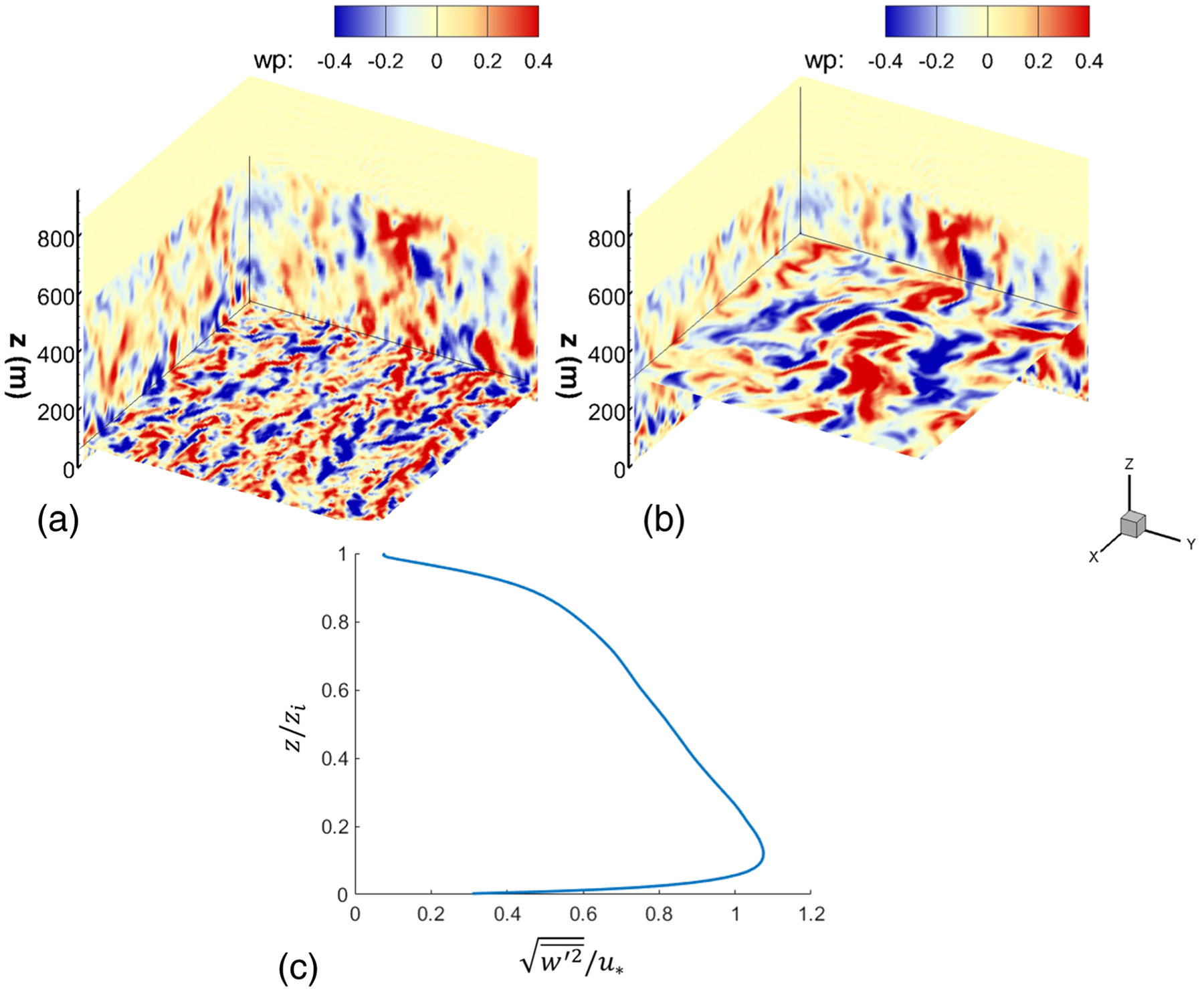
Snapshot of instantaneous vertical velocity with horizontal planes at (a) 100 m (z/zinv = 0.18) and (b) 300 m (z/zinv = 0.53) for the neutral boundary layer. (c) The time-averaged vertical profile of root-mean-square vertical velocity normalized by u*, the friction velocity.
The vertical concentration profile of newly generated sea spray aerosol particles (over time τ) is measured in the LES to parameterize ΨI. For neutral stability, the value of τ is normalized by the neutral stratification timescale τneut = zinv/u* (u* is the friction velocity), which is around 2,000 s. We choose the normalized model time step τ/τneut = 0.25 (where τ = 500 s), which is sufficiently large such that the transition matrix displays temporal stationarity, but small enough such that a Markov chain is required to capture correlation between particle jumps. Figure 2 shows the vertical concentration profiles for τ/τneut = 0.25 generated for 20 different windows [nτ, (n + 1)τ] for particles with diameter 2, 10, and 50 μm. This profile reflects the distribution ΨI of the newly injected particles reported by the LES. Note that we have plotted all 20 distinct profiles for each aerosol particle diameter, but they are all nearly identical and hence appear as a single profile. This overlap indicates that the turbulence is statistically steady state based on the chosen τ. For all aerosol particle sizes, the majority of newly generated particles remains in the lower atmosphere, meaning that τ/τneut = 0.25 is not sufficiently long for particles to sample the entire boundary layer. Again, this temporal correlation is what necessitates the use of a Markov chain component of the random walk model.
Figure 2.
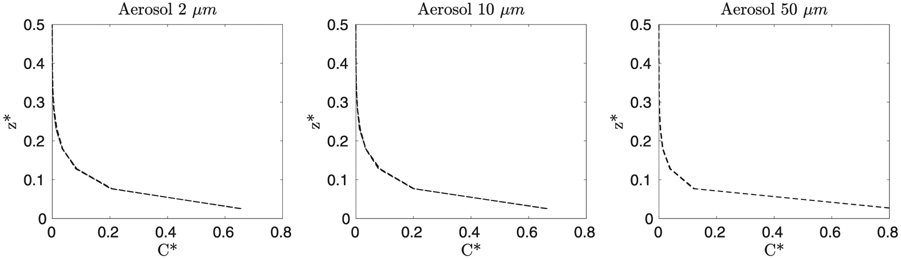
The distribution of newly generated aerosol particles ΨI from the LES in a τ/τneut = 0.25 window for neutral conditions. The y axis is the normalized vertical height z* = z/zinv, and the x axis is the normalized concentration C* = C(z)/CTot, where C(z) is the concentration of particles at a bin location, and CTot is the total concentration for a given snapshot. Twenty different temporal snapshots of ΨI are shown in each panel (but overlap).
As the diameter increases, the gravitational settling velocity increases, causing a higher concentration of particles near the surface as observed in Figure 2. Physically, larger particles require persistent and strong updrafts to reach the upper portions of the boundary layer, whereas smaller particles are more likely to reach greater heights and stay suspended without the need of constant upward velocities. Thus, larger particles exhibit lower concentrations as vertical height increases.
3.1.2. Markov Chain Random Walk Prediction
We apply the Markov chain random walk model to predict aerosol particle transport through the boundary layer and compare model predictions with the LES. Using the Lagrangian statistics, the transition matrix is parameterized, as shown in the top panels of Figure 3. As mentioned in section 2.2.1, the “start” and “transition” bins represent a spatial discretization of the atmospheric boundary layer. The rows represent all probabilities of transport from any given start bin to another bin (including its own same bin). For example, the probability of transport to bin 20 given being at bin 1 is very low (shown by the blue color), and its probability to remain at its same location (start bin 1, transition bin 1) is high. The position of an aerosol particle based on the normalized model time step τ/τneut = 0.25 is shows strong correlation based on its current position. Such behavior is captured by the transition matrices, which the colors (indicating probability) display strong diagonal trending; that is, particles that start at the bottom (or top) of the boundary layer are likely to stay at the bottom (or top).
Figure 3.
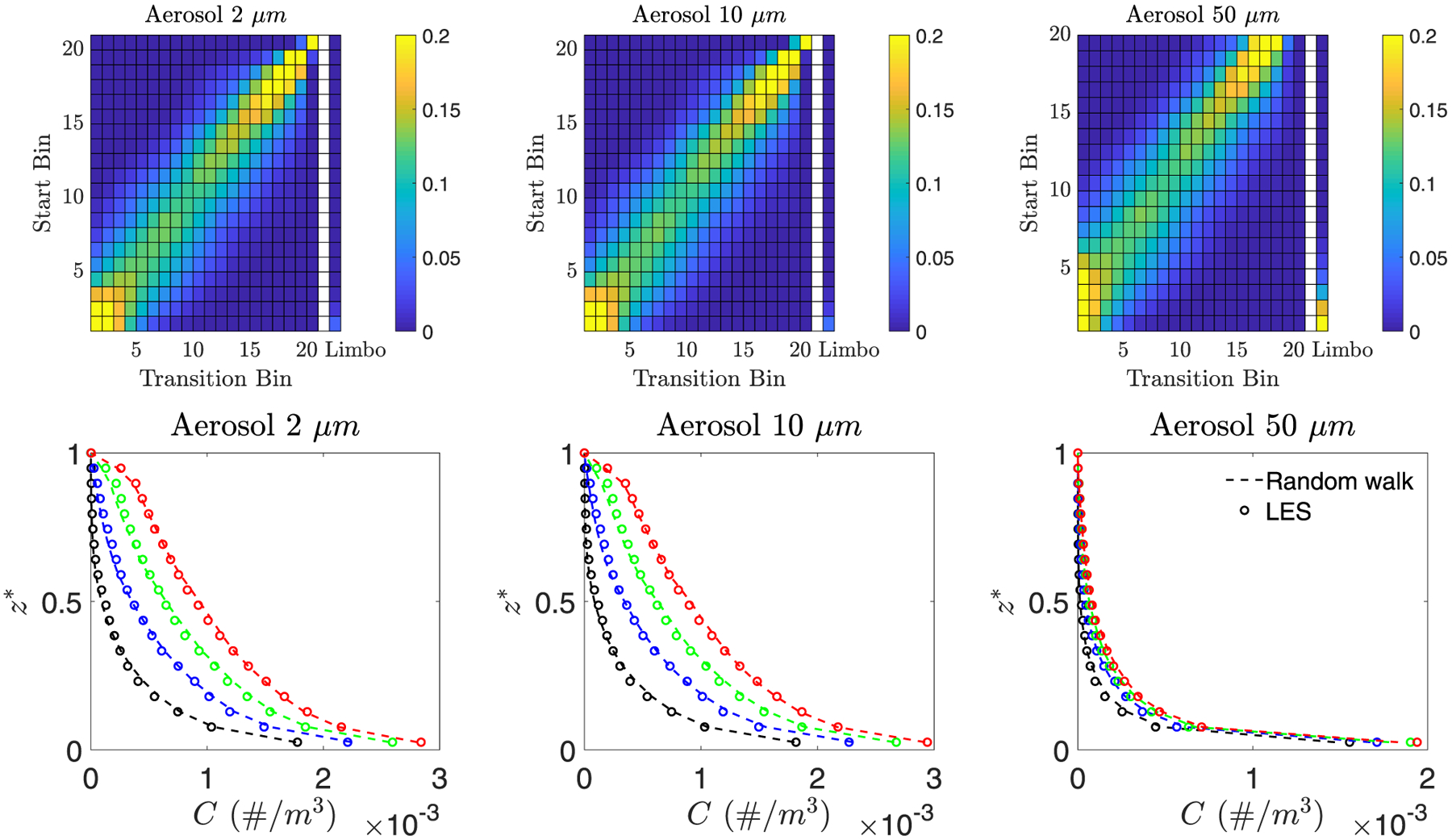
The top row shows transition matrices for particles with diameter d = 2,10, 50 μm with a normalized model time step τ/τneut = 0.25, where τ = 500 s, and the colors represent probability. The bottom row is the temporal evolution of the vertical aerosol particle concentration profiles in the neutral boundary layer for LES (dots) and the Markov chain upscaled model predictions (dashed line). The colors on the bottom row correspond to t/τneut = 1 (black), 2 (blue), 3 (green), and 4 (red), where t is the time since the first release of particles. Concentrations are provided as a local number density based on the number of particles in the LES.
For dry deposition to the surface, the rightmost column of the transition matrices quantifies the transition from some height to the ocean. As the distance between the ocean surface and current particle position decreases, the probability that the particle enters limbo (dry deposition) increases. Furthermore, as the particle’s diameter increases its probability of removal grows, seen as increased values in the removal column of the transition matrices—an effect well captured by the transition matrix and upscaled model.
Using this parameterization, the Markov chain model accurately represents the LES evolution of vertical concentration for 2, 10, and 50 μm diameter particles. Note that in contrast to C* shown in Figure 2, C is a dimensional number concentration given a local grid volume. Figure 3 shows the horizontally averaged concentration profile at snapshots of t/τneut = 1 (black), 2 (blue), 3 (green), and 4 (red) along the bottom row of panels, where t is the time since the first release of particles. As a reference, the reported concentrations are the number concentration from the LES given the injection rate (ϕs = 200 s−1). The atmosphere begins devoid of particles, and over time, the particle concentration increases as they are continuously injected at z = 0. As time evolves, particles have sufficient time to sample the full range of motions in the boundary layer, and turbulent dispersion results in the transport of particles throughout the boundary layer. For the d = 2,10 μm cases, turbulence is strong enough for such transport; however, in contrast, very few particles with a diameter of 50 μm make it to the top of the boundary layer because the turbulent field is too weak in comparison to gravitational settling. These features are well captured by the upscaled model.
3.2. Unstable (Convective) Boundary Layer
We now consider an unstable boundary layer in addition to the neutral conditions of the previous section. The surface heat flux in this scenario corresponds to a 1.5 K air-sea temperature difference, a typical setting over open oceans. In addition to the imposed geostrophic wind, buoyancy production of convective turbulence occurs due to the relatively warm surface. The significant amount of vertical mixing due to these convective motions causes a near-constant concentration with height, a feature in the profile which is very difficult for traditional 1-D analytical models to capture, as shown in N18.
3.2.1. Characterization of Unstable Boundary Layer
Figure 4 presents snapshots of vertical velocity with planes at two different heights, as well as a profile of vertical velocity fluctuations. Note that compared to Figure 1, the range of vertical velocity fluctuations are up to three times larger. In the wall-normal x-y planes, convective plumes are visible via large, coherent regions of vertical velocity fluctuation. These large-scale features are important to the transport of aerosol particles, as it will be shown to significantly affect the spatial probabilities displayed by the transition matrix. Additionally, the normalized root-mean-square of the vertical velocity shows the maximum of vertical mixing toward the center of the mixed layer, in agreement with other studies (Moeng & Sullivan, 1994).
Figure 4.
Snapshot of instantaneous vertical velocity with horizontal planes at (a) 100 m (z/zinv = 0.18) and (b) 300 m (z/zinv = 0.53) for the unstable boundary layer. (c) The time-averaged vertical profile of root-mean-square vertical velocity normalized by the convective velocity scale.
We use the standard definition of the convective velocity scale to define a convective large eddy timescale, τeddy = zinv/w*. Here, Ts is the reference surface temperature (273 K), is the surface heat flux, and g is gravitational acceleration. Our convective timescale is roughly 20 min, consistent with previous studies (Moeng & Sullivan, 1994). We first choose a model time step of τ = 500 s, which corresponds to τ/τeddy = 0.39. By choosing τ less than τeddy, the model time interval will be less than the time required to mix aerosols throughout the MABL, thus necessitating the Markov chain. Though it is possible to use the model step time τ/τeddy = 0.39 to make further step predictions past the model step time, we explore the Markov chain model capability for different model step times, particularly when larger than the greatest turbulent timescales. As the time step reaches the full range of turbulent timescales (~τ/τeddy > 1), we anticipate that this leads to temporal decorrelation. This decorrelation occurs when the transition matrix is equiprobable from any starting bin to any ending bin over the model time step. Thus, the larger timescale will remove the requirement of the Markov chain since particles would have enough time to sample the entire MABL. To test this, we also consider a case when τ is larger than τeddy: τ = 2,000 s, or τ/τeddy = 1.56. It will be shown that even in this case, the upscaled transport model can reasonably predict constant concentrations with height in the mixed layer.
Figure 5 displays ΨI for both τ/τeddy = 0.39 (top rows) and τ/τeddy = 1.56 (bottom rows). Each panel contains multiple profiles, representing different simulation windows from the LES of the corresponding normalized model time steps τ. Due to our simulation times ending at t = 1,1400 s, the model time step τ = 2,000 s allows for five unique instances of ΨI. In the neutral case, all ΨI are nearly identical; however, under unstable conditions, we observe that the profile of newly generated aerosol particles is somewhat variable in time. We attribute this variation to large-scale turbulent structures, which influence the convergence of time-averaged statistics. At the surface layer and inversion layer heights, the initial injection distributions are similar, where the large-scale structures are less dominant.
Figure 5.
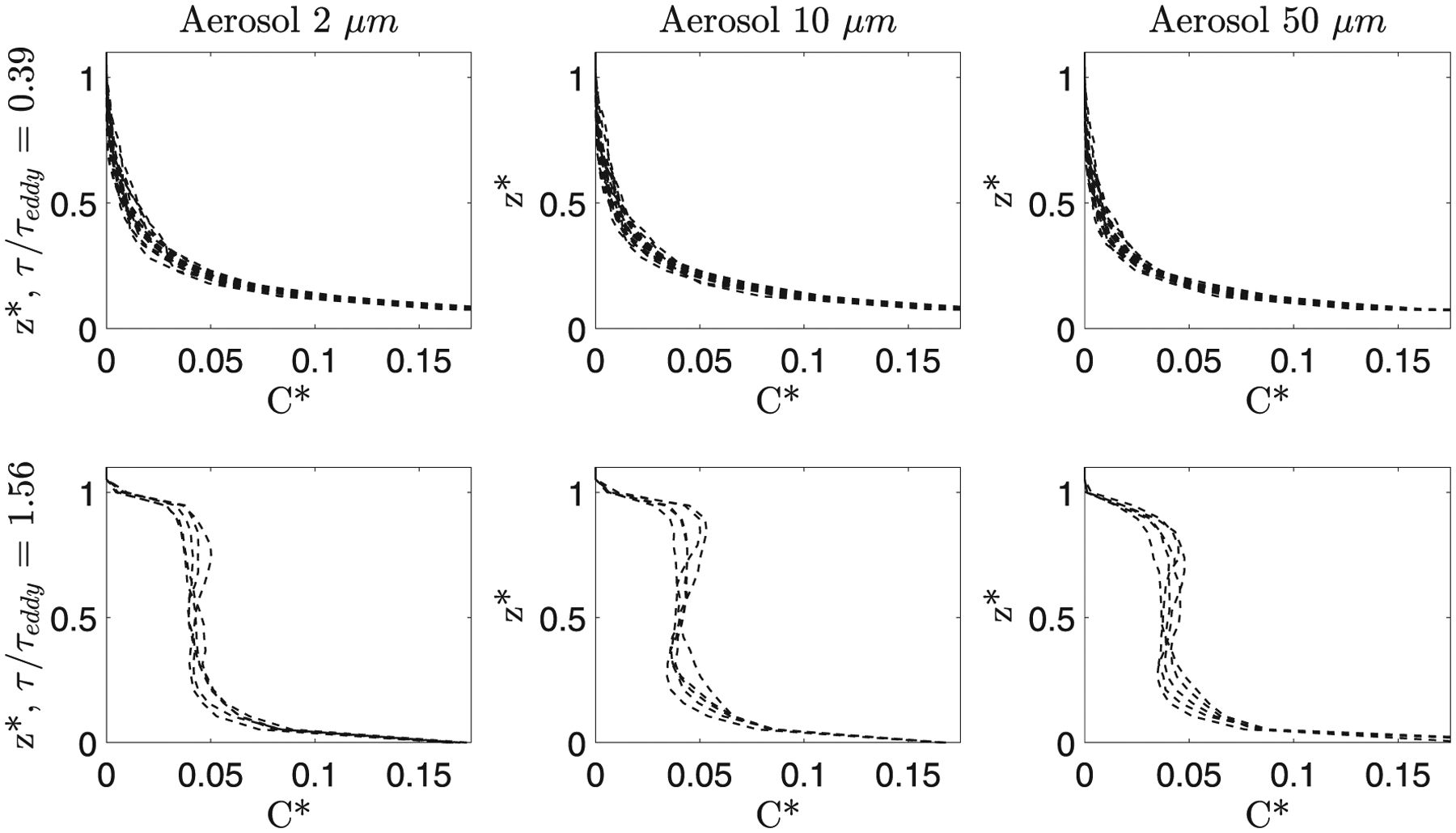
ΨI from the LES for two model time steps τ under unstable conditions. The top row represents τ/τeddy = 0.39, while the bottom row represents τ/τeddy = 1.56. The concentration is normalized in the same way as the neutral condition. Five snapshots are shown for τ = 2,000 s, demonstrating the temporal variability of the initial condition.
As expected, τ/τeddy = 0.39 displays concentrations that are able to reach the upper half of the boundary layer, unlike the neutral ΨI. Particle concentration is the largest in the surface layer, because aerosols are generated at the surface and are carried downwards by gravity—again, this becomes stronger with particle size. We choose the first profile, that is, the vertical concentration profile at t = τ, as the injection initial condition ΨI for both values of τ. For the case with τ = 2,000 s, the profile ΨI looks similar to the fully developed concentration profile, as expected since the particles have had sufficient time to distribute and sample the entire MABL.
3.2.2. Markov Chain Random Walk
We apply the same methodology of using the LES to determine M and ΨI to parameterize the upscaled model. In this section we present two random walk simulations using the two values of τ for the unstable boundary layer, and note the difference in vertical concentration predictions.
For unstable stratification, the transition matrix when using τ/τeddy = 0.39 is shown in the top row of Figure 6 and exhibits generally weak correlation throughout the mixed layer as compared to the neutral boundary layer (top rows of Figure 3). Preferential particle displacement relative to its original location is greater toward the surface and the inversion layer, where particles tend to remain for successive time intervals.
Figure 6.
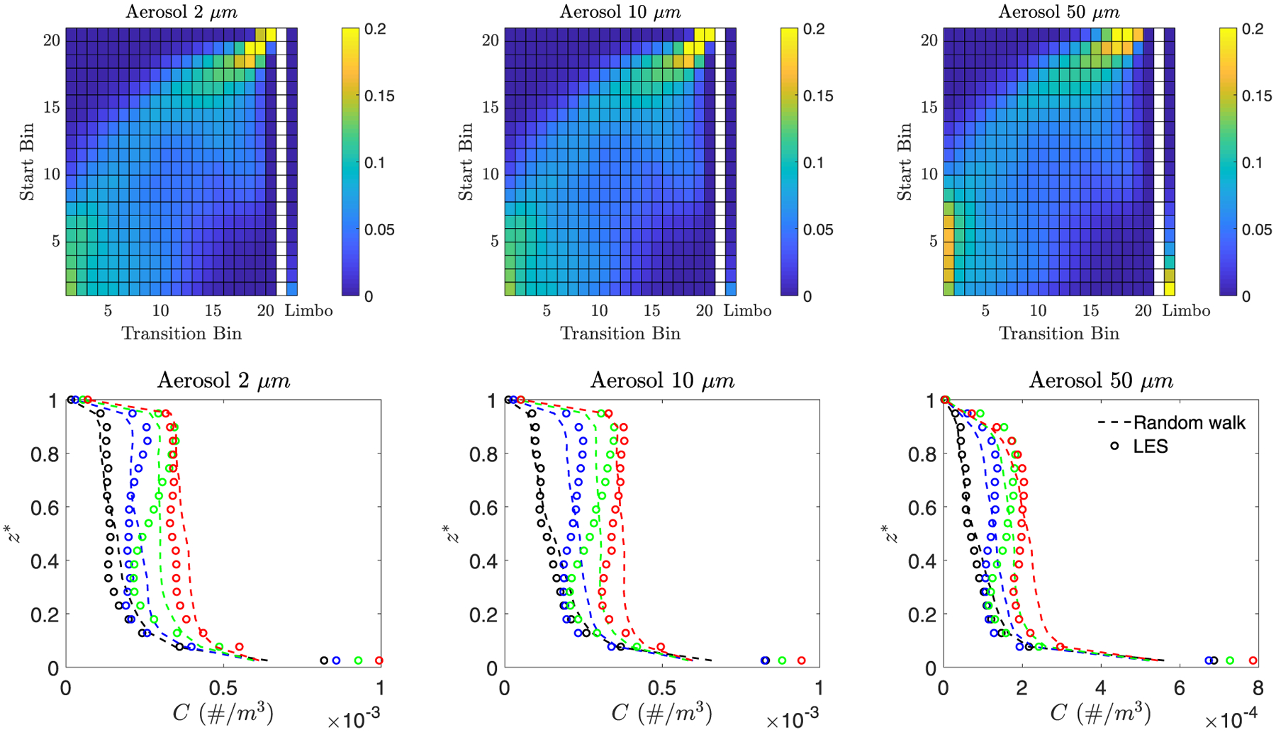
Transition matrices are shown above for particles with diameter d = 2,10, 50 μm using the normalized model time step τ/τeddy = 0.39, where τ = 500 s. The bottom panels are the temporal evolution of the vertical aerosol particle concentration profiles in the unstable boundary layer for LES (dots) and Markov chain upscaled model predictions (dashed lines). The random walk concentration is the scaled concentration with respect to the LES (see section 3.1.2). Colors correspond to t/τeddy = 0.39 (black), 0.78 (blue), 1.17 (green), and 1.56 (red), where t is the time since the first release of particles.
When using these transition matrices, the bottom rows of Figure 6 compare the model predictions to the LES results. Above a height of z/zi ≈ 0.2, the random walk model correctly predicts a near-uniform concentration profile, due to the enhanced vertical mixing relative to the neutral boundary layer. As noted above, it is this feature, which is very difficult for traditional eddy diffusivity models to capture. As the concentration of aerosols grows in the boundary layer, the Markov chain random walk model generally exhibits an under-prediction within the surface layer. Compared to the neutral case shown in Figure 3, there is more variation in the predictions for the unstable case, which is consistent with that seen in the profiles of ΨI and reflects the time variability of the horizontally averaged concentration. Similarly, the transition matrix at multiple instances of τ/τeddy = 0.39 undergoes slight temporal variation (not shown), but the general features remain the same since the flow is statistically stationary.
When setting τ/τeddy = 1.56 (τ = 2,000 s), the transition matrices reflect the well-mixed behavior exhibited in the concentration profiles, displayed in the top panels of Figure 7. As expected, the matrices are nearly uniform, meaning that a particle’s initial position is not important to the particle’s final position since the model time step τ is larger than the convective timescale. We again observe that increasing the aerosol particle size increases the probability that a particle enters limbo within the interval τ, and the probability of particle limbo is larger in the selection of τ/τeddy = 1.56 than in τ/τeddy = 0.39.
Figure 7.
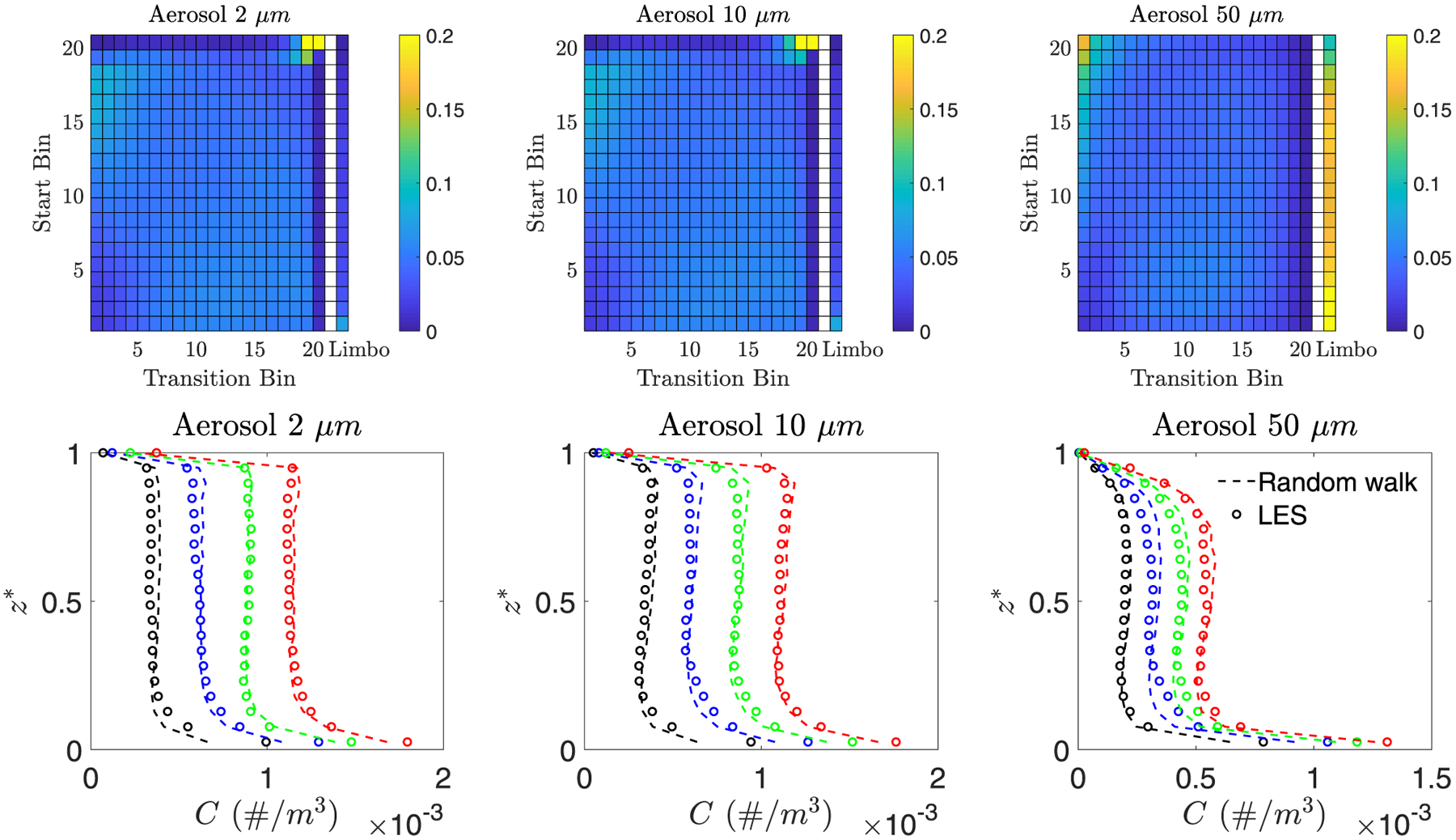
Transition matrices are shown below for particles with diameter d = 2,10, 50 μm using the normalized model time step τ/τeddy = 1.56, where τ = 2,000 s. The bottom panels are the temporal evolution of the vertical aerosol particle concentration profiles in the unstable boundary layer for LES (dots) and Markov chain upscaled model predictions (dashed line). Colors correspond to t/τeddy = 1.56 (black), t/τeddy = 3.13 (blue), t/τeddy = 4.69 (green), and t/τeddy = 6.25 (red).
When using τ/τeddy = 1.56, for all particle sizes the random walk model accurately captures the evolution of mean aerosol concentration; this is shown in the bottom panels of Figure 7. As mentioned above, τ/τeddy = 1.56 now takes into account the largest convective timescale. Once considering this timescale, the Markov chain near completely decorrelates over this time interval (within the surface and mixed layer), eliminating the need of a Markov chain and transition matrix formulation. Effectively, the injection initial condition of the random walk (ΨI) contains all of the information needed to make predictions, since it captures the shape of the well-mixed concentration profile.
4. Extended Analysis
With the initial results of the vertical concentration profile predictions for all considered particle sizes and stabilities, we can now expand upon analysis of the Markov chain random walk model. As mentioned before, the random walk model currently requires M and ΨI, which are obtained from the LES. With the goal of reducing computational cost associated with running LES, we begin this discussion by inferring new transition matrices based on already-calculated transition matrices—that is, from several matrices M calculated from LES of a limited set of particle sizes, M for other particle sizes can be predicted without needing additional LES.
With an eye on removing the need for using LES in total, we also discuss the possibility of using 1-D theory on particle distribution to specify ΨI and discuss the sensitivity of the model predictions to M in order to assess how robust the predictions of C would be to various (future) parameterizations of M. Lastly, the model output is compared with airborne field data and a global aerosol model to highlight its utility as a parameterization for subgrid schemes of large-scale models.
4.1. Inference of M Based on Particle Size
So far, we have shown predictions for models that were parameterized from the LES directly, meaning that we have full access to highly detailed Lagrangian trajectory data. However, such parameterization methods still require LES (albeit for much shorter durations) and therefore demand potentially large computational resources. In other words, we still need to simulate transport in order to predict transport, which somewhat defeats the purpose of upscaled modeling. In this section we use the previously calculated transition matrix data to infer how the transition matrix changes with aerosol particle size. Doing so means we can parameterize random walk models for a large range of particle sizes by gathering statistics from just a few LES cases, thereby reducing the computational costs associated with the parameterization step.
To demonstrate, we infer the transition matrix of a particle with diameter 35 μm from the transition matrices observed for particles with diameters 2, 5, 10, 20, 50 μm for the unstable and neutral boundary layers. To do so requires an adjustment of the probability of each transition matrix element with respect to particle size. Anticipating that the elements of the transition matrix scale with particle mass based on gravitational settling, thus depending on , we find a least squares best fit polynomial of degree 3; this reflects that the transition matrix elements are a function of particle volume. We find the best fit probability for every transition matrix element and then normalize rows, such that their summation is unity. The top graphs of Figure 8 display the best fit lines for the probability of the limbo state bin for the lowest five initial bins (distinguished by color), showing clearly that as particle radius increases, particle deposition becomes more likely at any bin. The best fit lines allow the probability of a transition matrix element to be estimated for any particle radius or diameter.
Figure 8.
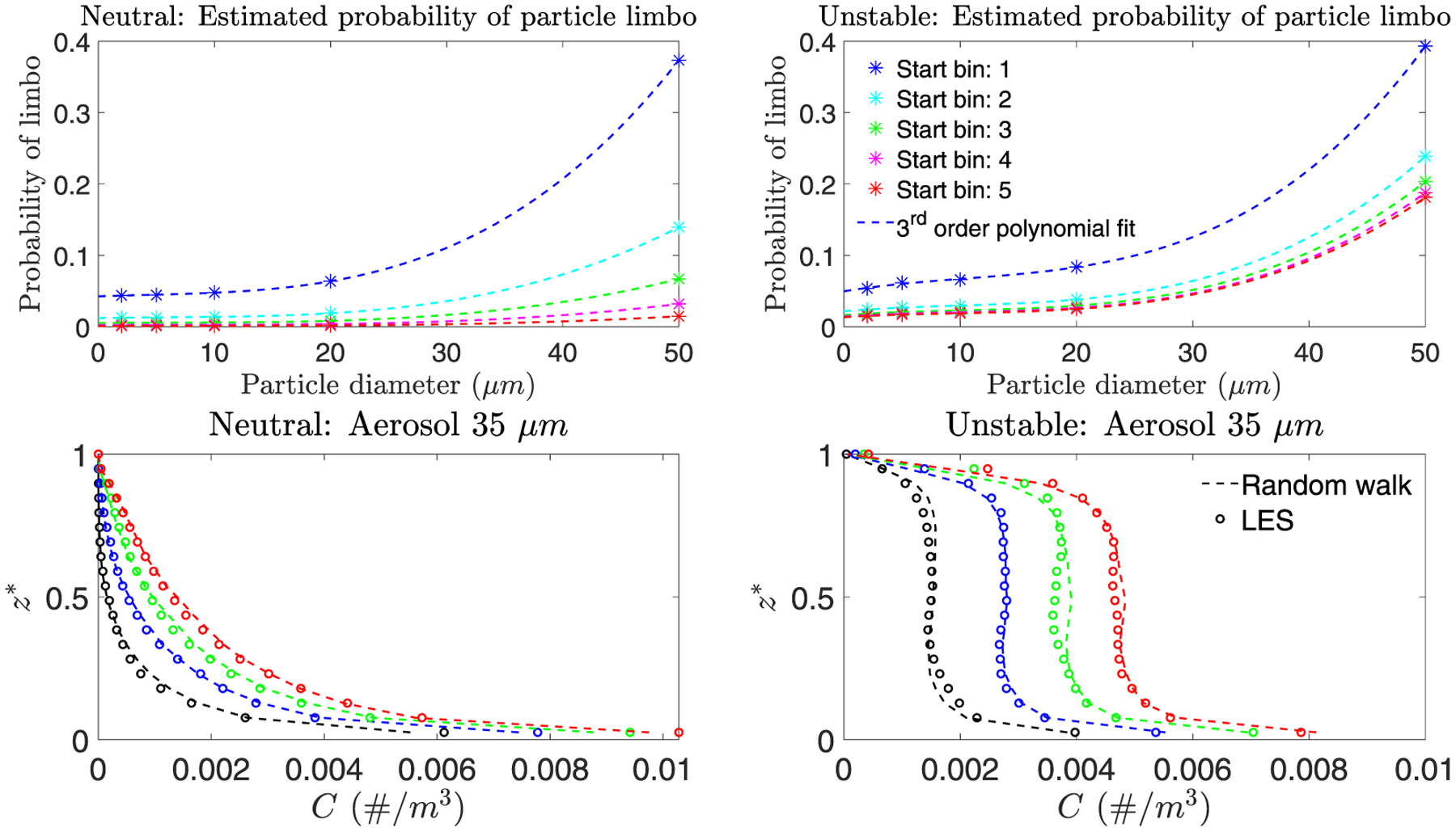
The top row shows the particle radius versus probability of limbo state and a best fit third-order polynomial for different atmospheric bins which are distinguished by color. The best fit polynomial is used to infer the transition matrix with diameter 35 μm. A transition matrix for an aerosol particle with a 35 μm diameter is inferred from transition matrices with other particle diameters. The temporal evolution of the concentration profiles from Markov chain model predictions (dashed lines) are compared with LES (dots) for the neutral (left) and unstable (right) cases. The temporal evolution (distinguished by color) is the same time stamps as Figure 3. The same setup is used as Figure 7 for the unstable case.
Once the transition matrix is inferred for a particle diameter of 35 μm, the random walk model is used to estimate the evolution of the vertical concentration profile under the same forcing conditions as presented earlier. In order for better convergence of Lagrangian statistics, we set ϕs = 600/s. The injection function ΨI for the 35 μm particles is obtained from the LES and used as the input parameter in the upscaled model. For both the neutral and unstable boundary layers, the Markov chain model accurately captures the LES behavior shown in the bottom panels of Figure 8. Here our simple interpolation method provides robust results, suggesting that the dependence of the transition matrix on particle can be approximated, restricting the need for full LES runs to only a subset of particle size. Additionally, the predictions demonstrate that the difference in ϕs has little to no effect, suggesting that the particle statistics have converged.
4.2. Comparison to a 1-D Analytical Model
In this section we compare a previously developed, 1-D analytical model with the LES results, in an effort to highlight the advantages of the proposed model. Specifically, we replicate vertical concentration profiles from the work of N18. In their model, the vertical gradient of mean concentration is calculated from the advection-diffusion equation for a passive scalar with a constant settling velocity, under the assumptions of horizontal homogeneity, negligible molecular diffusivity, zero mean vertical velocity, turbulent vertical flux parameterized with an eddy diffusivity, and a total (turbulent plus settling) vertical flux that decreases linearly with height from a constant surface flux Φ to 0 at zinv. The final equation can be written as
| (8) |
where C is the mean concentration and Kc(z) is the eddy diffusivity.
In addition to the physical parameters that are constant in the simulation (u*, zinv, ws, Φ, and the Obukhov length L), Equation 8 requires a model for the eddy diffusivity Kc(z), proposed by N18 as
| (9) |
where κ is the Von Kármán constant and ϕ(ζ) is the stability function for a passive scalar in the surface layer (ζ = z/L). This model extends the Monin-Obukhov similarity theory from the surface layer (Freire et al., 2016) to the entire ABL, through the use of a transitioning constant a = 1/(1 − 0.1zinv/zinv)2.
Figure 9 shows the comparison between N18’s model and the LES results for the same cases evaluated with the Markov chain random walk model. Although no explicit time is shown in Equation 8, the analytical solution varies in time because the reference concentration Cr (taken here as the surface concentration) changes in time: The theory assumes that the vertical profile is self-similar in its relationship between flux, surface concentration, and C(z).
Figure 9.
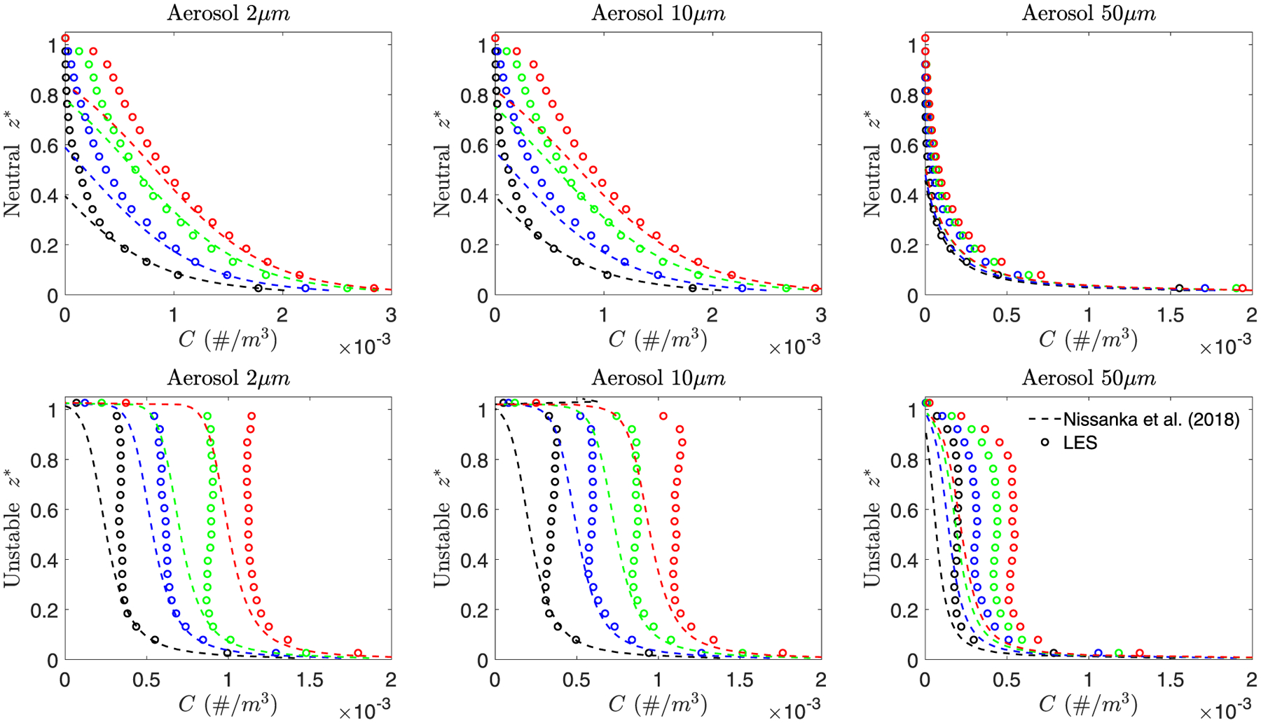
The temporal evolution of the vertical aerosol particle concentration profiles in the both neutral and unstable conditions for LES (dots) and 1-D analytical model proposed by Nissanka et al. (2018) (dashed lines) for particles with diameter d = 2,10, 50 μm for τ/τneut = 0.25 and τ/τeddy = 1.56 observation windows. The model time step is τ = 500 s for the neutral condition, and τ = 2,000 s for the unstable condition. Colors correspond to t/τneut = 1.0 and t/τeddy = 1.56 (black), t/τneut = 2.0 and t/τeddy = 3.13 (blue), t/τneut = 3.0 and t/τeddy = 4.69 (green), and t/τneut = 4.0 and t/τeddy = 6.25 (red).
In both neutral and unstable cases, the analytical model matches the simulation at the surface layer for particles with diameters of 2 and 10 μm. For the 50 μm case, physical processes that are not taken into account by the analytical model (such as the trajectory-crossing effect) start to be relevant, and the model is not expected to work (Csanady, 1963; Freire et al., 2016). In addition, the behavior at the upper part of the atmosphere is likely affected by the strong inversion and the accumulation of particles, which is also not considered in the theoretical model. Finally, as noted by N18, the well-mixed behavior of the unstable cases cannot be well represented by an eddy diffusivity approach (Stull, 1988; Wyngaard, 2010).
The random walk model is not constrained by the same assumptions and can easily adapt to different conditions, as long as they are embedded in the estimation of the transition matrix M and an accurate representation of ΨI. The critical case of well-mixed conditions is a clear example of this flexibility. The analytical model, on the other hand, is currently limited by the gradient diffusion approach to the turbulent transport parameterization. In addition, it does not consider the transient period during which aerosol particle growth occurs in the MABL, as explained in N18. Thus, this new approach has the potential to go beyond the limitations of the 1-D analytical model, making it worth the pursuit of parameterizations for M and ΨI.
4.3. The Use of 1-D Analytical Models as ΨI for the Neutral Boundary Layer
In the previous analyses, we used LES to parameterize the Markov chain random walk model inputs, M and ΨI. Here, we discuss another effort to de-link the training of the proposed model with the use of LES. Namely, we demonstrate that a theoretically derived surface layer profile can instead be used for the injection initial condition ΨI in the neutral ABL case. We use the model provided by Kind (1992) (hereafter referred to as K92), which corresponds to the mean concentration profile in the atmospheric surface layer (ASL) under steady-state and horizontally homogeneous conditions:
| (10) |
where C is again the horizontal mean concentration, Cr is the reference concentration at the reference height zr, Φ is the net concentration flux at the surface, and γ = τpg/κu* is the Rouse number (Rouse, 1937).
As shown in Figure 2, nearly all of the concentration remains within the surface layer (z ≤ 0.1zi) for a time interval of τ/τneut = 0.25, a situation that allows the application of an ASL model such as K92’s equation as an initial condition to the Markov chain random walk model. In this calculation, performed for τ/τneut = 0.25, the transition matrix used is the same as in previous analysis for the neutral ABL (section 3.1.2).
In Figure 10, concentration profiles calculated from the LES are compared to the Markov chain random walk model with an injection initial condition retrieved by K92’s analytical model. The use of the theoretical profile as ΨI in the neutral boundary layer continues to provide accurate predictions when comparing to the LES, especially for the 2 and 10 μm particle sizes. There exists a significant loss in predictive accuracy using the analytical model for 50 μm particles where the ASL model struggles, resulting in overprediction at nearly all heights.
Figure 10.
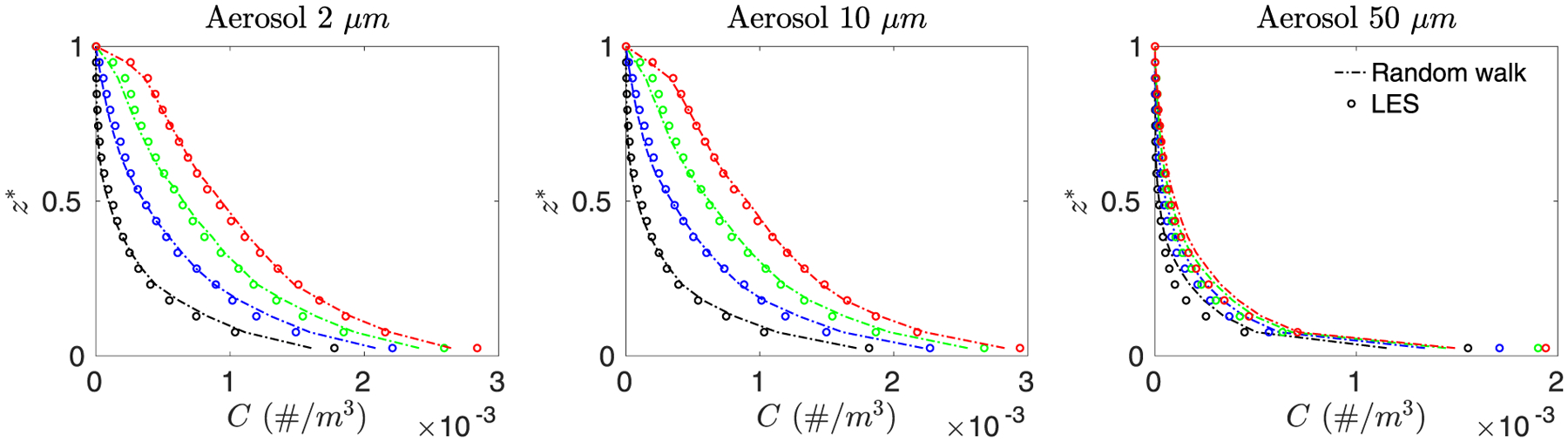
The temporal evolution of the vertical aerosol particle concentration profiles in the neutral case for the LES (dots), and using ΨI based on Kind (1992) with the random walk model (dashed lines) for particles with diameter d = 2,10, 50 μm. Colors correspond to t/τneut = 1 (black), 2 (blue), 3 (green), and 4 (red).
Thus, it is clearly important for the initial injection condition ΨI to be representative of the distribution of continually sourced aerosol particles. If ΨI does not capture the general particle transport features of the boundary layer, the predictions of the random walk model will have large errors even if M is perfect. As shown in Figure 9, in the unstable case the theoretical profiles have low accuracy above the surface layer, causing corresponding large errors in the random walk results if used as ΨI (not shown). Additionally, the use of τ/τeddy = 0.39 causes an even larger mismatch for the 1-D analytical model prediction for the unstable case. As mentioned in N18, the initial transient period is not taken into consideration, it will not accurately predict the aerosol particle growth in the boundary layer until these deficiencies are mitigated.
4.4. Upscaled Model Sensitivity and Limitations
In this study the considered model time steps, τ/τneut = 0.25 for the neutral case and two model time steps for the unstable case, τ/τeddy = 0.39 and τ/τeddy = 1.56, were demonstrated to accurately predict transport behavior. When τ → 0, particles do not have sufficient time for transport to other atmospheric height classes, meaning the transition matrix would have values of 1 along the diagonal and 0 otherwise; clearly, such a large transition probabilities would not accurately predict particle transport. When τ becomes much greater than the largest characteristic timescales of the flow, particle displacement over successive steps becomes increasingly decorrelated with each other (as observed in the unstable case with τ/τeddy = 1.56), and assuming independence over successive model steps becomes more valid. This removes the need for a Markov chain. As τ → ∞, all particles hit the ocean surface and are removed from the system, while being replaced by particles in the same location according to ΨI. Physically, this case represents a steady-state concentration of aerosol particles, though in the atmosphere this is rarely realized (Hoppel et al., 2005; Reid et al., 2001).
If the probabilities of the transition matrix are modified, then the prediction of the vertical concentration profiles will have a different outcome. At the same time, the importance of the transition matrix decreases as the model time step τ increases. Conversely, as τ becomes shorter, the prediction will become more sensitive to the structure (and any manipulation) of the transition matrix. The sensitivity of predicted concentration profiles based on changes of the transition matrix remains an open question, and in this section our goal is to test this sensitivity in order to ensure that the model performance is robust. Additionally, this information can provide insight for a baseline parameterization for M. To do this, we run the random walk model with transition matrices whose elements have been artificially manipulated.
For the neutral case in section 3.1.2, we consider a single particle size (10 μm), and again note that the transition matrix exhibits strong diagonal trending. Therefore, we adjust the probability that a particle remains in its current height class (i.e., the diagonal elements of the transition matrix) to 0%, 50%, and 150% of its actual value. Once the diagonal elements are adjusted, each row is normalized so its sum is unity.
In Figure 11, the temporal evolution of the concentration profiles for the same τ is displayed for the random walk model whose transition matrices have been artificially adjusted. The ΨI profile remains the same as the analysis done in section 3.1.2. For all adjustments in the transition bins, the 10 μm diameter vertical profiles maintain an accurate prediction compared to the LES simulations. With no likelihood that a particle stays at the same height (left figures), and also for that with a higher probability (right figures), the random walk model loses little accuracy in the prediction of concentration profiles. Slight overprediction occurs at later time steps in regions of large concentration (i.e., the surface layer), whereas in regions of lower concentrations (i.e., the inversion layer), the model underpredicts. Therefore, the Markov chain random walk model demonstrates a level of robustness based on the biased training of the transition matrix.
Figure 11.
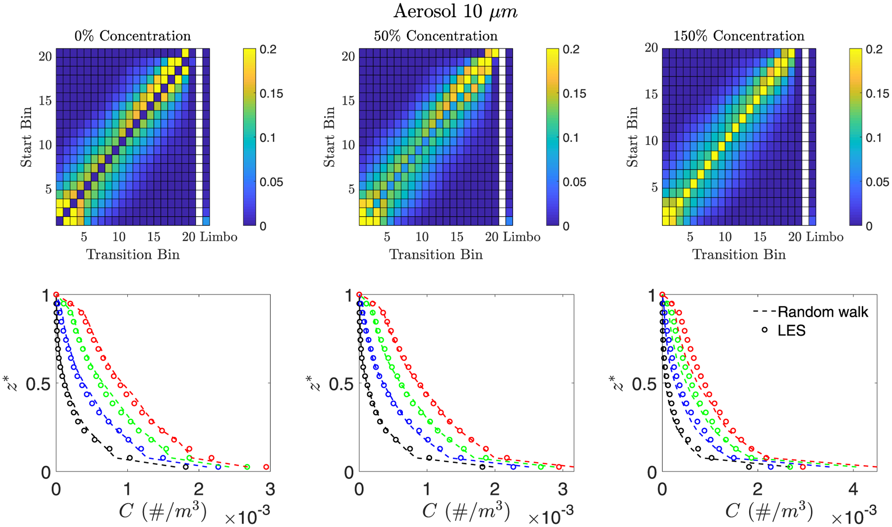
The temporal evolution of the vertical aerosol particle concentration profiles in neutral conditions for d = 10 μm. Associated transition matrices are shown above for adjusted diagonal probabilities of 0%, 50%, and 150%. The incremental t/τeddy are the same as in Figure 3.
For testing the sensitivity in the unstable stratification case, we perform a different manipulation of the transition matrix. The physical mechanisms of particle dispersion are fundamentally different in neutral versus unstable stratification, which can be seen in the differences between the transition matrices in section 3. The transition matrix of the unstable case approaches uniform transition probabilities more quickly with an increasing τ and particles are more subject to be transported large vertical distances; we therefore choose a different manipulation of the transition matrix to test robustness. Knowing that the transition matrix is nearly fully decorrelated when τ/τeddy = 1.56 (except at the inversion and surface deposition shown in Figure 7), we create a uniform transition matrix (top row of Figure 12).
Figure 12.
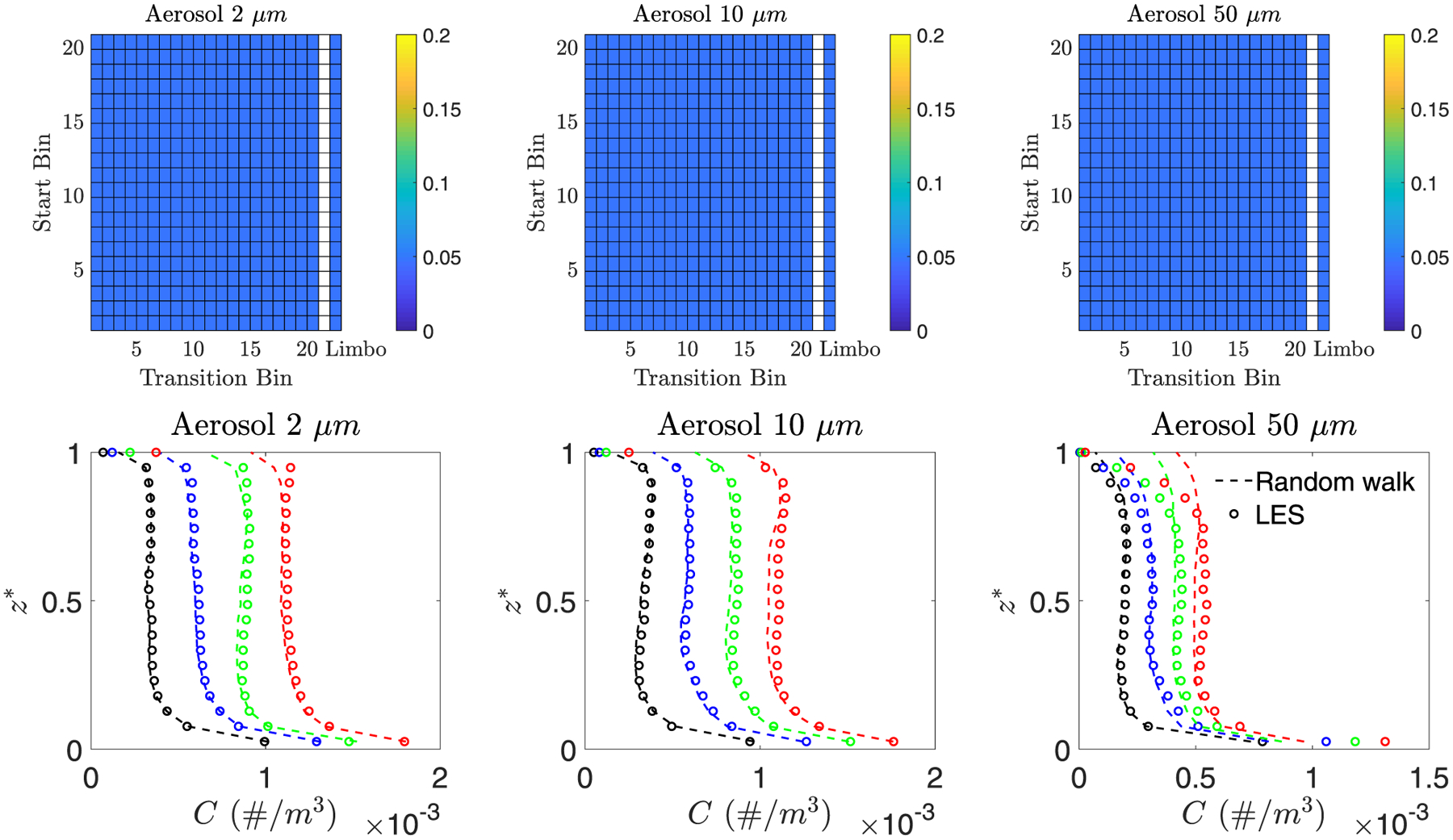
The temporal evolution of the vertical aerosol particle concentration profiles in an unstable stratification for a uniform transition matrix. The times t/τeddy are the same as in Figure 7.
A uniform matrix assumes particle transport that is independent of its original position, which occurs when all spatiotemporal scales of turbulent transport is trained into the transition matrix, as mentioned in section 2.2. In Figure 12, the temporal evolution of the concentration profiles are presented for the modified transition matrices in the unstable case. Visually, the probability of the transition matrices looks comparable to that of Figure 4, except at the inversion layer height as well as the limbo probability bin. Removal of the unstable correlation structure of the transition matrix affects the predictions at the top of the MABL, as concentrations become slightly over predicted. However, the profiles, as a whole, maintain accurate predictions in time, and again, the random walk model appears robust to modifications of the transition matrix. As a result, for a sufficiently large timescale τ, a baseline for the parameterization of M can be used as a uniform matrix for the unstable case with only a slight loss in accuracy at the inversion layer. This leads to the injection initial condition ΨI being of upmost importance in the parameterization of the Markov chain model for cases of decorrelated transition matrices, since in this limit it simply reflects the probability distribution of particles in space at each step.
4.5. Application to a Global Aerosol Model and Field Observations
Finally, to highlight the utility of the Markov chain random walk model, we compare its concentration profile predictions to that of a set of recent field observations and the prediction of an operational global aerosol model. The main goal of this section is to provide examples in which the upscaled model can be a tool for the global and perhaps mesoscale modeling community. We begin with the field study introduced by Schlosser et al. (2020) (hereafter referred to as S20), called the MONterey Aerosol Research Campaign (MONARC), where 14 repeated, identical flights were conducted from the California coast over the open ocean using the Center for Remotely Piloted Aircraft Studies (CIRPAS) Twin Otter aircraft. Flights consisted of repeated stair-stepping maneuvers to cycle between the following levels in order: near-surface (<60 m), below cloud base, just above cloud base, midcloud, just below cloud top, just above cloud top, ~150 m above cloud top, followed by a slant descent back to the near-surface level. On cloud-free days, stair stepping was similarly conducted with three levels sampled below the MABL top, followed by two above it, and then a slant descent back to the lowest level. A goal of the flights was to spatiotemporally characterize sea salt aerosol number concentrations and other variables. Supermicrometer (dry particle diameter [dp > 1 μm]) sea salt aerosol particles were measured with wing-mounted probes, providing number concentration at multiple heights. The most relevant probe is the Cloud and Aerosol Spectrometer (CAS), which measured size distributions for the ambient dp range between 0.76 and 75.80 μm. Schlosser et al. (2020) describe the method used to convert those data into dry dp values as the CAS conducted measurements at ambient relative humidity conditions.
At the same time, we obtain concentration profiles at the same location and time of the MONARC flights from the Navy Aerosol and Analysis Prediction System (NAAPS) (Lynch et al., 2016); it is a forecasting aerosol model driven by meteorological data from the Navy Global Environmental Model (NAVGEM; Hogan et al., 2014). Sea salt is assumed as tracer particles and their dry mass concentrations is forecasted. The physical processes that are applied to sea salt are emission from the surface, wind-based dispersion and advection, and removal from the atmosphere by wet and dry deposition (Witek et al., 2007). We specifically consider two sets of data obtained on 4 June 2020 and 6 June 2020, which both display qualities of an unstably stratified atmosphere. The reader is referred to S20 for a more detailed description of the synoptic and meteorological conditions during these two flights.
In order to make comparisons between our Markov chain random walk model, the MONARC observations, and the NAAPS predictions, we must make certain assumptions. First, we assume that the stratification in the atmosphere during the research flights is similar to our baseline unstable case. This is based on the air-sea temperature difference and TKE levels reported in S20, and we inherently assume that the transition matrix of our unstable case is not sensitive to stability parameters as long as it is in the unstable regime. Second, we assume that the transport of all dp > 1 μm particles can be represented in our model with a monodisperse, dp = 2 μm distribution. This is based primarily on the report in S20 that the volume median diameter of the MONARC flights was 1.80 and 2.60 μm for 4 and 6 June, respectively. Polydisperse concentrations could straightforwardly be used in the Markov chain model, but we use monodisperse for simplicity here. Assuming a monodisperse distribution furthermore allows us to convert between number and mass concentrations for comparison purposes.
We take the transition matrix from the case with τ/τeddy = 1.56, predict concentrations, and compare it directly to the measured concentrations from 4 and 6 June. Figure 13 shows the normalized concentration profiles of S20 (4 and 6 June), the Markov chain random walk model, and NAAPS (4 and 6 June). The concentrations of all three profiles are normalized using the concentration at the center of the boundary layer. The data from S20 exhibit well-mixed, constant concentrations with height; this feature is not completely tracked by predictions of NAAPS, which overpredict concentrations at the lowest few grid points. It is generally understood that marine aerosol concentrations increase near the surface (Blanchard et al., 1984; Woodcock, 1953); however, this layer can be very thin and difficult to resolve at coarse resolution. The Markov chain random walk model well captures the shape of the measured aerosol distribution, although it has not been presently trained to accurately predict aerosol transport above the boundary layer top since the aerosol concentration has been assumed to be 0 during the development of the transition matrix. By combining the fast, accurate aerosol distribution provided by the Markov chain random walk model with the bulk predictions of NAAPS, more accurate predictions of boundary layer concentrations (and the inherent fine-scale gradients) can likely be achieved even in atmospheric models with coarse resolution.
Figure 13.
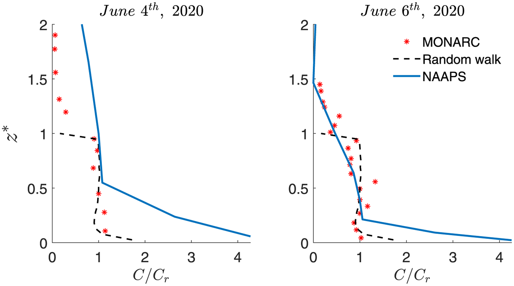
Nondimensional concentration profiles from S20 (red dots), Markov chain random walk (dashed lines), and NAAPS (blue line). Concentrations are normalized by Cr, the concentration at the boundary layer midpoint, and heights are normalized by the boundary layer height.
5. Conclusions
In the present study we model the evolution of vertical aerosol particle concentrations for unstable and neutral boundary layer conditions over a range of particle sizes. To do so, we introduce an upscaled random walk model, and LES is used as a testbed for comparison and informing upscaled model parameters. In order to accurately predict transport behavior, the boundary conditions and the physical processes that govern transport must be effectively upscaled. All of the physical processes related to vertical transport of aerosols considered by the LES are captured in a Markov chain random walk model. The benefit of this approach is that once parameterized, the new model is approximately 1 million times faster than using the LES model (calculated via cpu hours).
In the model framework, particles vertically transition through the MABL by random walk, which is enforced with a transition matrix. Hence, particle trajectories are modeled as a temporal Markov process. We test the upscaled model robustness by predicting the evolution of vertical concentration profiles for varying stability conditions and particle diameters. For all cases, the upscaled model faithfully represents transport behavior observed in the high fidelity LES. In comparison, 1-D analytical models cannot take into account the transient accumulation of aerosol particles in the MABL, and also cannot obtain constant concentrations with height in an unstably stratifed environment (Nissanka et al., 2018). We demonstrate that for the neutral case, 1-D analytical models can be used to parameterize the injection initial condition ΨI of our proposed upscaled model without degrading prediction accuracy. Finally, the model, namely, the transition matrix, is manipulated to explore its sensitivity and limitations. This information provides a basis for parameterization of M.
An outstanding challenge to the proposed modeling framework is the parameterization of the transition matrix without using LES. Currently, a major problem is that in order to predict transport behavior, transport first must be simulated. This has been a common problem in the subsurface hydrology community. However, recent advances have been made in analytic Markov models (Kang et al., 2015; Morales et al., 2017), inverse modeling approaches (Sherman et al., 2017, 2018), and assumes that correlations in time are governed by well-known stochastic processes, such as Bernoulli or Ornstein-Uhlenbeck (Dentz et al., 2016; Hyman et al., 2019; Sherman et al., 2020). In addition, the transition matrix is versatile for many particle dispersion problems: Its parameterization does not strictly depend on any particle transport assumptions (such as being a dilute or nonevaporating), as long as it is temporally stationary. We envision that with some future effort similar methodologies may be applied in the context of the proposed MABL model and that our work here motivates such advances.
Furthermore, the designation of τ in the training of the transition matrix is still somewhat arbitrary, only as long as temporal stationarity is satisfied. In this study, the normalized random walk time step τ/τneut = 0.25 (T = 500 s) for the neutral condition showed strong correlation, a feature well captured by the transition matrix. For the unstable boundary layer, the use of τ/τeddy = 0.39 showed weaker probabilistic particle displacement, attributed by the large-scale convective structures of turbulence. Increasing the normalized model time step to τ/τeddy = 1.56 shows that the transition matrix is effectively uniform past the timescale of one large-scale eddy life cycle, relaxing the necessity of the Markov chain to the random walk model for model prediction. Once specific τ values are determined, the upscaled Markov random walk serves as a computationally efficient subgrid model that can be implemented in current boundary layer representation in global aerosol models.
Key Points:
The proposed model replicates LES outputs for multiple particle sizes and two atmospheric states
Particle displacement is found to vary between the two atmospheric states based on a model time step
The model demonstrates potential upgrade and utility for coarser-scale weather and climate models
Acknowledgments
H. P., G. W., and D. R. were supported by the Office of Naval Research (ONR) under Grant No. N00014-16-1-2472 and the Army Research Office under Grant No. G00003613-ArmyW911NF-17-0366. L. F. was funded by São Paulo Research Foundation (FAPESP, Brazil) Grant No. 2018/24284-1. Computational resources were provided by the Notre Dame Center for Research Computing. T. S. is supported by the National Science Foundation Graduate Research Fellowship under Grant No. DGE-1841556. Authors P. X. and J. S. R.’s contributions were supported by the Office of Naval Research Code 322 and the NRL Base Program. Author A. S.’s contributions were funded by the Office of Naval Research grant N00014-16-1-2567 and National Aeronautics and Space Administration (NASA) grant 80NSSC19K0442, the latter of which is in support of the ACTIVATE Earth Venture Suborbital-3 (EVS-3) investigation, which is funded by NASA’s Earth Science Division and managed through the Earth System Science Pathfinder Program Office. We also give thanks to the data provided by the Navy global aerosol model (NAAPS).
Footnotes
Data Availability Statement
Markov chain random walk data presented in this work can be found online (https://doi.org/10.5281/zenodo.3703180). MONARC data can be accessed at Sorooshian et al. (2017) (https://doi.org/10.6084/m9.figshare.5099983.v10) and are described in detail by Sorooshian et al. (2018).
References
- Andreas EL (1998). A new spray generation function for wind speeds up to 32 m/s. Journal of Physical Oceanography, 28(11), 10 [DOI] [Google Scholar]
- Balachandar S, & Eaton JK (2010). Turbulent dispersed multiphase flow. Annual Review of Fluid Mechanics, 42(1), 111–133. 10.1146/annurev.fluid.010908.165243 [DOI] [Google Scholar]
- Berkowitz B, Cortis A, Dentz M, & Scher H (2006). Modeling non-Fickian transport in geological formations as a continuous time random walk. Reviews of Geophysics, 44, RG2003 10.1029/2005RG000178 [DOI] [Google Scholar]
- Bian H, Froyd K, Murphy DM, Dibb J, Chin M, Colarco PR, et al. (2019). Observationally constrained analysis of sea salt aerosol in the marine atmosphere. Atmospheric Chemistry and Physics Discussions, 19, 10,773–10,785. 10.5194/acp-19-10773-2019 [DOI] [Google Scholar]
- Blanchard DC, Woodcock AH, & Cipriano RJ (1984). The vertical distribution of the concentration of sea salt in the marine atmosphere near Hawaii. Tellus B, 36 B(2), 118–125. 10.1111/j.1600-0889.1984.tb00233.x [DOI] [Google Scholar]
- Bolster D, Méheust Y, Le Borgne T, Bouquain J, & Davy P (2014). Modeling preasymptotic transport in flows with significant inertial and trapping effects—The importance of velocity correlations and a spatial markov model. Advances in Water Resources, 70, 89–103. 10.1016/j.advwatres.2014.04.014 [DOI] [Google Scholar]
- Brennen CE (2005). Fundamentals of multiphase flow. Cambridge University Press. [Google Scholar]
- Caffrey PF, Hoppel WA, & Shi JJ (2006). A one-dimensional sectional aerosol model integrated with mesoscale meteorological data to study marine boundary layer aerosol dynamics. Journal of Geophysical Research, 111, D24201 10.1029/2006JD007237 [DOI] [Google Scholar]
- Chamecki M, Hout R, Meneveau C, & Parlange MB (2007). Concentration profiles of particles settling in the neutral and stratified atmospheric boundary layer. Boundary-Layer Meteorology, 125(1), 25–38. 10.1007/s10546-007-9194-5 [DOI] [Google Scholar]
- Clarke AD, Owens SR, & Zhou J (2006). An ultrafine sea-salt flux from breaking waves: Implications for cloud condensation nuclei in the remote marine atmosphere. Journal of Geophysical Research, 111, D06202 10.1029/2005JD006565 [DOI] [Google Scholar]
- Csanady GT (1963). Turbulent diffusion of heavy particles in the atmosphere. Journal of the Atmospheric Sciences, 20(3), 201–208. [DOI] [Google Scholar]
- De Anna P, Le Borgne T, Dentz M, Tartakovsky AM, Bolster D, & Davy P (2013). Flow intermittency, dispersion, and correlated continuous time random walks in porous media. Physical Review Letters, 110(18), 184502 10.1103/PhysRevLett.110.184502 [DOI] [PubMed] [Google Scholar]
- de Leeuw G, Neele FP, Hill M, Smith MH, & Vignati E (2000). Production of sea spray aerosol in the surf zone. Journal of Geophysical Research, 105(D24), 29,397–29,409. 10.1029/2000JD900549 [DOI] [Google Scholar]
- Deardorff JW (1972). Numerical investigation of neutral and unstable planetary boundary layers. Journal of the Atmospheric Sciences, 29, 91–115. [DOI] [Google Scholar]
- Deardorff JW (1980). Stratocumulus-capped mixed layers derived from a three dimensional model. Boundary-Layer Meteorology, 18(4), 495–527. 10.1007/BF00119502 [DOI] [Google Scholar]
- Delay F, Ackerer P, & Danquigny C (2005). Simulating solute transport in porous or fractured formations using random walk particle tracking: A review. Vadose Zone Journal, 4(2), 360–379. 10.2136/vzj2004.0125 [DOI] [Google Scholar]
- Dentz M, Kang PK, Comolli A, Le Borgne T, & Lester DR (2016). Continuous time random walks for the evolution of Lagrangian velocities. Physical Review Fluids, 1(7), 074004. [Google Scholar]
- Erickson DJ, Seuzaret C, Keene WC, & Gong SL (1999). A general circulation model based calculation of HCl and ClNO2 production from sea salt dechlorination: Reactive chlorine emissions inventory. Journal of Geophysical Research, 104(D7), 8347–8372. 10.1029/98JD01384 [DOI] [Google Scholar]
- Freire LS, Chamecki M, & Gillies JA (2016). Flux-profile relationship for dust concentration in the stratified atmospheric surface layer. Boundary-Layer Meteorology, 160(2), 249–267. 10.1007/s10546-016-0140-2 [DOI] [Google Scholar]
- Gerber H (1991). Supersaturation and droplet spectral evolution in fog. Journal of the Atmospheric Sciences, 48(24), 2569–2588. [DOI] [Google Scholar]
- Ghan SJ, Guzman G, & Abdul-Razzak H (1998). Competition between sea salt and sulfate particles as cloud condensation nuclei. Journal of the Atmospheric Sciences, 55(22), 3340–3347. [DOI] [Google Scholar]
- Giuggioli L, Sevilla FJ, & Kenkre VM (2009). A generalized master equation approach to modelling anomalous transport in animal movement. Journal of Physics A: Mathematical and Theoretical, 42(43), 434004 10.1088/1751-8113/42/43/434004 [DOI] [Google Scholar]
- Hogan TF, Liu M, Ridout JA, Peng MS, Whitcomb TR, Ruston BC, et al. (2014). The navy global environmental model. Oceanography, 27(3), 116–125. [Google Scholar]
- Hoppel WA, Caffrey PF, & Frick GM (2005). Particle deposition on water: Surface source versus upwind source. Journal of Geophysical Research, 110, D10206 10.1029/2004JD005148 [DOI] [Google Scholar]
- Hyman JD, Dentz M, Hagberg A, & Kang PK (2019). Linking structural and transport properties in three-dimensional fracture networks. Journal of Geophysical Research: Solid Earth, 124, 1185–1204. 10.1029/2018JB016553 [DOI] [Google Scholar]
- Kang PK, Le Borgne T, Dentz M, Bour O, & Juanes R (2015). Impact of velocity correlation and distribution on transport in fractured media: Field evidence and theoretical model. Water Resources Research, 51, 940–959. 10.1002/2014WR015799 [DOI] [Google Scholar]
- Kind RJ (1992). One-dimensional aeolian suspension above beds of loose particles-A new concentration-profile equation. Atmospheric Environment Part A, General Topics, 26(5), 927–931. 10.1016/0960-1686(92)90250-O [DOI] [Google Scholar]
- Klemp JB, & Durran DR (1983). An upper boundary condition permitting internal gravity wave radiation in numerical mesoscale models. Monthly Weather Review, 111(3), 430–444. [DOI] [Google Scholar]
- Lamb RG (1978). A numerical simulation of dispersion from an elevated point source in the convective planetary boundary layer. Atmospheric Environment, 12(6–7), 1297–1304. 10.1016/0004-6981(78)90068-9 [DOI] [Google Scholar]
- Le Borgne T, Dentz M, & Carrera J (2008). Lagrangian statistical model for transport in highly heterogeneous velocity fields. Physical Review Letters, 101(9), 090601 10.1103/PhysRevLett.101.090601 [DOI] [PubMed] [Google Scholar]
- Lewis ER, & Schwartz SE (2004). Sea salt aerosol production: Mechanisms, methods, measurements, and models—A critical review. Washington, DC: American Geophysical Union. [Google Scholar]
- Liang T, Chamecki M, & Yu X (2016). Sea salt aerosol deposition in the coastal zone: A large eddy simulation study. Atmospheric Research, 180, 119–127. 10.1016/j.atmosres.2016.05.019 [DOI] [Google Scholar]
- Lynch P, Reid JS, Westphal DL, Zhang J, Hogan TF, Hyer EJ, et al. (2016). An 11-year global gridded aerosol optical thickness reanalysis (v1.0) for atmospheric and climate sciences. Geoscientific Model Development, 9(4), 1489–1522. 10.5194/gmd-9-1489-2016 [DOI] [Google Scholar]
- Moeng C-H (1984). A large-eddy-simulation model for the study of planetary boundary-layer turbulence. Journal of the Atmospheric Sciences, 41(13), 2052–2062. [DOI] [Google Scholar]
- Moeng C-H, & Sullivan PP (1994). A comparison of shear- and buoyancy-driven planetary boundary layer flows. Journal of the Atmospheric Sciences, 51(7), 999–1022. [DOI] [Google Scholar]
- Moeng C-H, & Wyngaard JC (1988). Spectral analysis of large-eddy simulations of the convective boundary layer. Journal of the Atmospheric Sciences, 45(23), 3573–3587. [DOI] [Google Scholar]
- Montero M, & Masoliver J (2017). Continuous time random walks with memory and financial distributions. The European Physical Journal B, 90(11), 207 10.1140/epjb/e2017-80259-4 [DOI] [Google Scholar]
- Morales VL, Dentz M, Willmann M, & Holzner M (2017). Stochastic dynamics of intermittent pore-scale particle motion in three-dimensional porous media: Experiments and theory. Geophysical Research Letters, 44, 9361–9371. 10.1002/2017GL074326 [DOI] [Google Scholar]
- Nelson J (1999). Continuous-time random-walk model of electron transport in nanocrystalline TiO 2 electrodes. Physical Review B, 59(23), 15374 10.1103/PhysRevB.59.15374 [DOI] [Google Scholar]
- Nissanka ID, Park HJ, Freire LS, Chamecki M, Reid JS, & Richter DH (2018). Parameterized vertical concentration profiles for aerosols in the marine atmospheric boundary layer. Journal of Geophysical Research: Atmospheres, 123, 9688–9702. 10.1029/2018JD028820 [DOI] [PMC free article] [PubMed] [Google Scholar]
- Peng T, & Richter D (2019). Sea spray and its feedback effects: Assessing bulk algorithms of air-sea heat fluxes via direct numerical simulations. Journal of Physical Oceanography, 49(6), 1403–1421. 10.1175/JPO-D-18-0193.1 [DOI] [Google Scholar]
- Prandtl L (1981). Essentials of fluid dynamics. Blackie and Son, London. [Google Scholar]
- Quinn PK, Collins DB, Grassian VH, Prather KA, & Bates TS (2015). Chemistry and related properties of freshly emitted sea spray aerosol. Chemical Reviews, 115(10), 4383–4399. 10.1021/cr500713g [DOI] [PubMed] [Google Scholar]
- Reid JS, Jonsson HH, Smith MH, & Smirnov A (2001). Evolution of the vertical profile and flux of large sea-salt particles in a coastal zone. Journal of Geophysical Research, 106(D11), 12,039–12,053. 10.1029/2000JD900848 [DOI] [Google Scholar]
- Reid JS, Reid EA, Walker A, Piketh S, Cliff S, Mandoos AA, et al. (2008). Dynamics of southwest Asian dust particle size characteristics with implications for global dust research. Journal of Geophysical Research, 113, D14212 10.1029/2007JD009752 [DOI] [Google Scholar]
- Richter DH, Dempsey AE, & Sullivan PP (2019). Turbulent transport of spray droplets in the vicinity of moving surface waves. Journal of Physical Oceanography, 49(7), 1789–1807. 10.1175/JPO-D-19-0003.1 [DOI] [Google Scholar]
- Riemer N, Vogel H, Vogel B, & Fiedler F (2003). Modeling aerosols on the mesoscale-γ: Treatment of soot aerosol and its radiative effects. Journal of Geophysical Research, 108(19). 10.1029/2003JD003448 [DOI] [Google Scholar]
- Rouse H (1937). Modern conceptions of the mechanics of fluid turbulence. American Society of Civil Engineers Transactions, 102, 463–505. [Google Scholar]
- Scalas E (2006). The application of continuous-time random walks in finance and economics. Physica A: Statistical Mechanics and its Applications, 362(2), 225–239. 10.1016/j.physa.2005.11.024 [DOI] [Google Scholar]
- Schlosser JS, Dadashazar H, Edwards E, Hossein Mardi A, Prabhakar G, Stahl C, et al. (2020). Relationships between supermicrometer sea salt aerosol and marine boundary layer conditions: Insights from repeated identical flight patterns. Journal of Geophysical Research: Atmospheres, 125, e2019JD032346 10.1029/2019JD032346 [DOI] [PMC free article] [PubMed] [Google Scholar]
- Sherman T, Fakhari A, Miller S, Singha K, & Bolster D (2017). Parameterizing the spatial Markov model from breakthrough curve data alone. Water Resources Research, 53, 10,888–10,898. 10.1002/2017WR021810 [DOI] [Google Scholar]
- Sherman T, Foster A, Bolster D, & Singha K (2018). Predicting downstream concentration histories from upstream data in column experiments. Water Resources Research, 54, 9684–9694. 10.1029/2018WR023420 [DOI] [Google Scholar]
- Sherman T, Hyman J, Dentz M, & Bolster D (2020). Characterizing the influence of fracture density on network scale transport. Journal of Geophysical Research: Solid Earth, 125, e2019JB018547 10.1029/2019JB018547 [DOI] [Google Scholar]
- Sherman T, Roche KR, Richter DH, Packman AI, & Bolster D (2019). A dual domain stochastic lagrangian model for predicting transport in open channels with hyporheic exchange. Advances in Water Resources, 125, 57–67. 10.1016/j.advwatres.2019.01.007 [DOI] [Google Scholar]
- Shi H, & Yu X (2015). An effective Euler-Lagrange model for suspended sediment transport by open channel flows. International Journal of Sediment Research, 30(4), 361–370. 10.1016/j.ijsrc.2015.03.012 [DOI] [Google Scholar]
- Sorooshian A, MacDonald AB, Dadashazar H, Bates KH, Coggon MM, Craven JS, et al. (2017). A multi-year data set on aerosol-cloud-precipitation-meteorology interactions for marine stratocumulus clouds. 10.6084/m9.figshare.5099983.v10 [DOI] [PMC free article] [PubMed]
- Sorooshian A, MacDonald AB, Dadashazar H, Bates KH, Coggon MM, Craven JS, et al. (2018). A multi-year data set on aerosol-cloud-precipitation-meteorology interactions for marine stratocumulus clouds. Scientific Data, 5, 180026. [DOI] [PMC free article] [PubMed] [Google Scholar]
- Stolaki S, Haeffelin M, Lac C, Dupont JC, Elias T, & Masson V (2015). Influence of aerosols on the life cycle of a radiation fog event. A numerical and observational study. Atmospheric Research, 151, 146–161. 10.1016/j.atmosres.2014.04.013 [DOI] [Google Scholar]
- Stull RB (1988). An introduction to boundary layer meteorology. Springer; Netherlands. [Google Scholar]
- Sullivan PP, Moeng C-H, Stevens B, Lenschow DH, & Mayor SD (1998). Structure of the entrainment zone capping the convective atmospheric boundary layer. Journal of the Atmospheric Sciences, 55(19), 3042–3064. [DOI] [Google Scholar]
- Sullivan PP, & Patton EG (2011). The effect of mesh resolution on convective boundary layer statistics and structures generated by large-eddy simulation. Journal of the Atmospheric Sciences, 68(10), 2395–2415. 10.1175/JAS-D-10-05010.1 [DOI] [Google Scholar]
- Sund NL, Bolster D, & Dawson C (2015). Upscaling transport of a reacting solute through a peridocially converging-diverging channel at pre-asymptotic times. Journal of Contaminant Hydrology, 182, 1–15. 10.1016/j.jconhyd.2015.08.003 [DOI] [PubMed] [Google Scholar]
- Toba Y (1965). On the giant sea-salt particles in the atmosphere I. General features of the distribution. Tellus, 17(1), 131–145. 10.3402/tellusa.v17i1.8997 [DOI] [Google Scholar]
- Van Kampen NG (1979). Composite stochastic processes. Physica A: Statistical Mechanics and its Applications, 96(3), 435–453. [Google Scholar]
- Veron F (2015). Ocean spray. Annual Review of Fluid Mechanics, 47, 507–538. 10.1146/annurev-fluid-010814-014651 [DOI] [Google Scholar]
- Winkler P (1988). The growth of atmospheric aerosol particles with relative humidity. Physica Scripta, 37(2), 223–230. 10.1088/0031-8949/37/2/008 [DOI] [Google Scholar]
- Witek ML, Flatau PJ, Quinn PK, & Westphal DL (2007). Global sea-salt modeling: Results and validation against multicampaign shipboard measurements. Journal of Geophysical Research, 112, D08215 10.1029/2006JD007779 [DOI] [Google Scholar]
- Woodcock AH (1953). Salt nuclei in marine air as a function of altitude and wind force. Journal of Meteorology, 10(5), 362–371. [DOI] [Google Scholar]
- Wyngaard JC (2010). Turbulence in the atmosphere. Cambridge University Press. [Google Scholar]
- Wyngaard JC, & Brost RA (1984). Top-down and bottom-up diffusion of a scalar in the convective boundary layer. Journal of the Atmospheric Sciences, 41(1), 102–112. [DOI] [Google Scholar]