A Projection-based Conditional Dependence Measure with Applications to High-dimensional Undirected Graphical Models

Abstract

Measuring conditional dependence is an important topic in econometrics with broad applications including graphical models. Under a factor model setting, a new conditional dependence measure based on projection is proposed. The corresponding conditional independence test is developed with the asymptotic null distribution unveiled where the number of factors could be high-dimensional. It is also shown that the new test has control over the asymptotic type I error and can be calculated efficiently. A generic method for building dependency graphs without Gaussian assumption using the new test is elaborated. We show the superiority of the new method, implemented in the R package pgraph, through simulation and real data studies.

1. Introduction

Rapid development in technology continuously floods us with high-dimensional data nowadays. One interesting question we wish to answer is their conditional dependency structure. Mathematically, let z = (z⁽¹⁾, …, z^(d)) be a d-dimensional random vector, which represents our data. We would like to know whether $z^{\left(i\right)}⫫z^{\left(j\right)}|\mathbf{\text{z}}\backslash \left\{z^{\left(i\right)},z^{\left(j\right)}\right\}$ for $i\ne j\in \left\{1,\dots ,d\right\}$ or if there are other factors f associated with z, then whether $z^{\left(i\right)}⫫z^{\left(j\right)}|\mathbf{\text{f}}$. For visualization, a graph is often used to represent such a conditional dependence structure: vertices represent observed variables and edges indicate conditional dependence. Producing such a graph can help us understand data and has been an important topic in fields including economics, finance, signal processing, bioinformatics and network modeling (Wainwright and Jordan, 2008).

Intrinsically, if we look at the nodes pair by pair, this is a testing problem. In general, we can write our goal as testing whether x and y are independent given f, i.e.,

$$H_0:\mathbf{\text{x}}⫫\mathbf{\text{y}}|\mathbf{\text{f}},$$ (1)

where x, y and f are random vectors with possibly different dimensions. For such conditional independence tests, there has been abundant literature, especially in econometrics. Linton and Gozalo (1997) proposed two nonparametric tests based on a generalization of the empirical distribution function; however, a complicated bootstrap procedure is needed to calculate critical values of the test, which limits its applications. Su and White (2007, 2008, 2014) and Wang et al. (2015) proposed conditional independence tests based on Hellinger distance, empirical likelihood, conditional moments and conditional characteristic function, respectively. However, as many of the recently available datasets are of high-dimension, the computation for these tests becomes prohibitive. Another related work is Sen and Sen (2014), where the focus is on testing the independence between the error and the predictor variables in the linear regression problem.

Our starting point is a relatively “general” model on {x, y, f}. In particular, suppose $\left\{\left({\text{x}}_i,{\text{y}}_i,{\text{f}}_i,{ϵ}_{i,x},{ϵ}_{i,y}\right),i=1,\dots ,n\right\}$ are i.i.d. realizations of $\left(\text{x},\text{y},\text{f},{ϵ}_x,{ϵ}_y\right)$, which are generated from the following model:

$$\text{x}={\mathit{G}}_x\left(\text{f}\right)+{ϵ}_x,\hspace{1em}\text{y}={\mathit{G}}_y\left(\text{f}\right)+{ϵ}_y,$$ (2)

where f is the K-dimensional common factors, G_x and G_y are general mappings from ${ℝ}^K$ to ${ℝ}^p$ and ${ℝ}^q$, respectively. The observed data are {(x_i, y_i, f_i), i = 1, …, n}. Here, for simplicity and tractability, we assume independence between (ϵ_x, ϵ_y) and f. Such kind of models shed light for another route to solve the issues, nonparametric regression. The idea is intuitive: to test (1) is the same as testing ${ϵ}_x⫫{ϵ}_y$ under (2), which naturally leads to a two-step procedure. Since {(ϵ_i,x, ϵ_i,y), i = 1, …, n} are not observed, in Step 1, we estimate the residuals. In this regard, we assume the dimensions p and q to be fixed while the number of factors K could diverge to infinity. Step 2, we apply an independence test on the estimated residuals. These two steps constitute our new conditional independence test and we will unveil the asymptotic properties for this new test statistic. Let’s briefly preview the procedure in the following two paragraphs.

In Step 1, ideally, a fully nonparametric projection on f (e.g., local linear regression (Fan, 1992)) would consistently recover the random errors asymptotically under certain smoothness assumptions on G_x and G_y, when K is fixed. However, it becomes challenging when K diverges due to the curse of dimensionality if no structural assumptions are made on G_x and G_y. As a result, in this paper, we will study two cases where G_x and G_y are linear functions (factor models) in Section 2.2 and where G_x and G_y are additive functions in Section 2.5 when K diverges. Further relaxed models might be available for future work, but we don’t focus on them in this paper.

To complete our proposal, after estimating the residuals in Step 1, we still need to find a suitable measure of dependence between random variables/vectors in Step 2. In this regard, many different measures of dependence have been proposed. Some of them rely heavily on Gaussian assumptions, such as Pearson correlation, which measures linear dependence and the uncorrelatedness is equivalent to independence only when the joint distribution is Gaussian; or Wilks Lambda (Wilks, 1935), where normality is adopted to calculate the likelihood ratio. To deal with non-linear dependence and non-Gaussian distribution, statisticians have proposed rank-based correlation measures, including Spearman’s ρ and Kendall’s τ, which are more robust than Pearson correlation against deviations from normality. However, these correlation measures are usually only effective for monotonic types of dependence. In addition, under the null hypothesis that two variables are independent, no general statistical distribution of the coefficients associated with these measures has been derived. Other related works include Hoeffding (1948), Blomqvist (1950), Blum et al. (1961), and some methods described in Hollander et al. (2013) and Anderson (1962). Taking these into consideration, distance covariance (Székely et al., 2007) was introduced to address these deficiencies. The major benefits of distance covariance are: first, zero distance covariance implies independence, and hence it is a true dependence measure. Second, distance covariance can measure the dependence between any two vectors which potentially are of different dimensions. Recently, Huo and Székely (2016) proposed a fast computation method for distance covariance. Due to these advantages, we will focus on distance covariance in this paper as our measure of dependence.

So far, we complete a rough description of the newly proposed conditional dependence measure; and we are able to build conditional dependency graphs by conducting this test edge by edge. We would like to make two remarks here to help readers connect the dots between our work and some other existing related topics/works.

First, let us look at the connection to undirected graphical models. Undirected graphical models (UGM) has been a popular topic in econometrics in the past decade. It studies the “internal” conditional dependency structure of a multivariate random vector. To be more explicit, again let z = (z⁽¹⁾, …, z^(d)) be the d-dimensional random vector of interest. We denote the undirected graph corresponding to z by (V, E), where vertices V correspond to components of z and edges E = {e_ij, 1 ≤ i ≠ j ≤ d} indicate whether node z⁽ⁱ⁾ and z^(j) are conditionally independent given the remaining nodes. In particular, the edge e_ij is absent if and only if $z^{\left(i\right)}⫫z^{\left(j\right)}|\text{z}\backslash \left\{z^{\left(i\right)},z^{\left(j\right)}\right\}$. Therefore, UGM is a nature application of our measure if we take f = z \ {z⁽ⁱ⁾, z^(j)} in our test. One intensively studied sub-field is GGM (Gaussian graphical model) where z is assumed to follow a multivariate Gaussian distribution with mean µ and covariance matrix Σ. This extra assumption is desirable since then the precision matrix Ω = (w_ij)_d×d = Σ⁻¹ captures exactly the conditional dependency graph; that is, w_ij = 0 if and only if e_ij is absent (Lauritzen, 1996; Edwards, 2000). Therefore, under the Gaussian assumption, this problem reduces to the estimation of precision matrix, where a rich literature on model selection and parameter estimation can be found in both low-dimensional and high-dimensional settings, including Dempster (1972), Drton and Perlman (2004), Meinshausen and Bühlmann (2006), Friedman et al. (2008), Fan et al. (2009), Cai et al. (2011), Liu (2013), Chen et al. (2014), Ren et al. (2015), Jankova and Van De Geer (2015) and Yu and Bien (2017). With simple derivations, it’s easy to check that GGM fits into our framework with G being linear and ϵ having Gaussian distributions. Therefore, with linear projection in Step 1 and distance covariance in Step 2, our proposed conditional measure solves GGM. It’s worth noting that, indeed, in Step 2, choosing Pearson correlation will solve GGM as well; choosing distance covariance gives more flexibility since we don’t assume normality on ϵ and potentially we can solve non-Gaussian UGMs. Another interesting work is Voorman et al. (2013), where a semi-parametric method was introduced for graph estimation.

Second, we examine the link to factor models. As explained in the last paragraph, UGM is a case with f being internal factors, in other words, part of the interested vector z. Another scenario of our framework is the case when f are external, and this is closely related to factor models. As an example, in the Fama-French three factors model, the excessive return of each stock can be considered as one node in the graph we want to build and f are the chosen three-factors. This example will be further elaborated in Section 5. Therefore, the factors f are considered as external since they are not part of the individual stock returns. Another interesting application is discussed in Stock and Watson (2002), where external factors are aggregated macroeconomic variables, and the nodes are disaggregated macroeconomic variables.

With the above two remarks, we see our proposed test cover some of the existing topics as by-products. We summarize the main contribution of this paper here. First, under model (2), we propose a computationally efficient conditional independence test. Both the response vectors and the common factors can be of different dimensions and the number of the factors could grow to infinity with sample size. Second, we apply this test to build conditional dependency graph (internal factors) and covariates-adjusted dependency graph (external factors).

The rest of this paper is organized as follows. In Section 2, we present our new procedure for testing conditional independence via projected distance covariance (P-DCov) and describe how to construct conditional dependency graphs based on the proposed test. Section 3 gives theoretical properties including the asymptotic distribution of the test statistic under the null hypothesis as well as the type I error guarantee. Section 4 contains extensive numerical studies and Section 5 demonstrates the performance of P-DCov via a financial data set. We conclude the paper with a short discussion in Section 6. Several technical lemmas and all proofs are relegated to the appendix.

2. Methods

2.1. A brief review of distance covariance

First, we introduce some notations. For a random vector z, ‖z‖ and ‖z‖₁ represent its Euclidean norm and ℓ₁ norm, respectively. A collection of n i.i.d. observations of z is denoted as {z₁, …, z_n}, where ${\text{z}}_k={(z_k^{\left(1\right)},\dots ,z_k^{\left(d\right)})}^T$ represents the k-th observation. For any matrix M, ‖M‖_F, ‖M‖ and ‖M‖_max denote its Frobenius norm, operator norm and max norm, respectively. ‖M‖_a,b is the (a, b) norm defined as the ℓ_b norm of the vector consisting of column-wise ℓ_a norm of M. Furthermore, a ∧ b represents min{a, b} and a ∨ b represents max{a, b}.

As an important tool, distance covariance is briefly reviewed in this section with further details available in Székely et al. (2007). We introduce several definitions as follows.

Definition 1. (w-weighted L₂ norm) Let $c_d=\frac{{\pi }^{\left(d+1\right)/2}}{\Gamma \left(\left(d+1\right)/2\right)}$, for any positive integer d, where Γ is the Gamma function. Then for function γ defined on ${ℝ}^p\times {ℝ}^q$, the w-weighted L₂ norm of γ is defined by

$${\Vert \gamma \left(\mathit{\tau },\mathit{\rho }\right)\Vert }_w^2={\int }_{{ℝ}^{p+q}}{\left|\gamma \left(\mathit{\tau },\mathit{\rho }\right)\right|}^{2}w\left(\mathit{\tau },\mathit{\rho }\right)d\mathit{\tau }d\mathit{\rho },\hspace{1em}where\hspace{0.17em}w\left(\mathit{\tau },\mathit{\rho }\right)={\left(c_p{c}_q{\Vert \mathit{\tau }\Vert }^{1+p}{\Vert \mathit{\rho }\Vert }^{1+q}\right)}^{-1}.$$

Definition 2. (Distance covariance) The distance covariance between random vectors $\text{x}\in {ℝ}^p$ and $\text{y}\in {ℝ}^q$ with finite first moments is the nonnegative number $\mathcal{V}\left(\text{x},\text{y}\right)$ defined by

$${\mathcal{V}}^2\left(\text{x},\text{y}\right)={\Vert g_{\text{x},\text{y}}\left(\mathit{\tau },\mathit{\rho }\right)-g_{\text{x}}\left(\mathit{\tau }\right)g_{\text{y}}\left(\mathit{\rho }\right)\Vert }_w^2,$$

where g_x, g_y and g_x,y represent the characteristic functions of x, y and the joint characteristic function of x and y, respectively.

Suppose we observe random sample {(x_k, y_k) : k = 1, …, n} from the joint distribution of (x, y). We denote X = (x₁, x₂, …, x_n) and Y = (y₁, y₂, …, y_n).

Definition 3. (Empirical distance covariance) The empirical distance covariance between samples X and Y is the nonnegative random variable ${\mathcal{V}}_n\left(\mathbf{\text{X}},\mathbf{\text{Y}}\right)$ defined by

$${\mathcal{V}}_n^2\left(\mathbf{\text{X}},\mathbf{\text{Y}}\right)=S_1\left(\mathbf{\text{X}},\mathbf{\text{Y}}\right)+S_2\left(\mathbf{\text{X}},\mathbf{\text{Y}}\right)-2S_3\left(\mathbf{\text{X}},\mathbf{\text{Y}}\right),$$

where

$$S_1\left(\mathbf{\text{X}},\mathbf{\text{Y}}\right)=\frac{1}{n^2}\sum _{k,l=1}^n\Vert {\mathbf{\text{x}}}_k-{\mathbf{\text{x}}}_l\Vert \Vert {\mathbf{\text{y}}}_k-{\mathbf{\text{y}}}_l\Vert ,\hspace{0.17em}\hspace{0.17em}{S}_2\left(\mathbf{\text{X}},\mathbf{\text{Y}}\right)=\frac{1}{n^2}\sum _{k,l=1}^n\Vert {\mathbf{\text{x}}}_k-{\mathbf{\text{x}}}_l\Vert \frac{1}{n^2}\sum _{k,l=1}^n\Vert {\mathbf{\text{y}}}_k-{\mathbf{\text{y}}}_l\Vert ,$$

$$S_3\left(\mathbf{\text{X}},\mathbf{\text{Y}}\right)=\frac{1}{n^3}\sum _{k=1}^n\sum _{l,m=1}^n\Vert {\mathbf{\text{x}}}_k-{\mathbf{\text{x}}}_l\Vert \Vert {\mathbf{\text{y}}}_k-{\mathbf{\text{y}}}_m\Vert .$$

With above definitions, Lemma 1 depicts the consistency of ${\mathcal{V}}_n\left(\mathbf{\text{X}},\mathbf{\text{Y}}\right)$ as an estimator of $\mathcal{V}\left(\mathbf{\text{x}},\mathbf{\text{y}}\right)$. Lemma 2 shows the asymptotic distribution of ${\mathcal{V}}_n\left(\mathbf{\text{X}},\mathbf{\text{Y}}\right)$ under the null hypothesis that x and y are independent. Corollary 1 reveals properties of the test statistic $n{\mathcal{V}}_n^2/S_2$ proposed in Székely et al. (2007).

Lemma 1. (Theorem 2 in Székely et al. (2007)) Assume that $\mathbb{E}\left(\Vert \text{x}\Vert +\Vert \text{y}\Vert \right)<\infty$, then almost surely

$$\underset{n\to \infty }{\text{lim}}{\mathcal{V}}_n\left(\text{X},\text{Y}\right)=\mathcal{V}\left(\text{x},\text{y}\right).$$

Lemma 2. (Theorem 5 in Székely et al. (2007)) Assume that x and y are independent, and $\mathbb{E}\left(\Vert \text{x}\Vert +\Vert \text{y}\Vert \right)<\infty$, then as n → ∞,

$$n{\mathcal{V}}_n^2\left(\text{X},\text{Y}\right)\stackrel{D}{\to }{\Vert \zeta \left(\mathit{\tau },\mathit{\rho }\right)\Vert }_w^2,$$

where $\stackrel{D}{\to }$ represents convergence in distribution and ζ(·, ·) denotes a complex-valued centered Gaussian random process with covariance function

$$R\left(\mathbf{\text{u}},{\mathbf{\text{u}}}_0\right)=\left(g_x\left(\mathit{\tau }-{\mathit{\tau }}_0\right)-g_x\left(\mathit{\tau }\right)\overline{g_x\left({\mathit{\tau }}_0\right)}\right)\left(g_y\left(\mathit{\rho }-{\mathit{\rho }}_0\right)-g_y\left(\mathit{\rho }\right)\overline{g_y\left({\mathit{\rho }}_0\right)}\right),$$

in which u = (τ, ρ), u₀ = (τ ₀, ρ₀).

Corollary 1. (Corollary 2 in Székely et al. (2007)) Assume that $\mathbb{E}\left(\Vert \text{x}\Vert +\Vert \text{y}\Vert \right)<\infty$.

1. If x and y are independent, then as n → ∞, $n{\mathcal{V}}_n^2\left(\text{X},\text{Y}\right)/S_2\left(\text{X},\text{Y}\right)\stackrel{D}{\to }Q$ with $Q\stackrel{D}{=}{\sum }_{j=1}^{\infty }{\lambda }_j{Z}_j^2$, where $Z_j\stackrel{i.i.d}{~}\mathcal{N}\left(0,1\right)$ and {λ_j} are non-negative constants depending on the distribution of (x, y);$\mathbb{E}\left(Q\right)=1$.

2. If x and y are dependent, then as n → ∞, $n{\mathcal{V}}_n^2\left(\text{X},\text{Y}\right)/S_2\left(\text{X},\text{Y}\right)\stackrel{P}{\to }\infty$.

2.2. Conditional independence test via projected distance covariance (P-DCov)

Here, we consider the case where G_x and G_y are linear in (2), which leads to the following factor model setup:

$$\mathbf{\text{x}}={\mathbf{\text{B}}}_x\mathbf{\text{f}}+{\mathit{ϵ}}_x,\hspace{1em}\mathbf{\text{y}}={\mathbf{\text{B}}}_y\mathbf{\text{f}}+{\mathit{ϵ}}_y,$$ (3)

where B_x and B_y are factor loading matrices of dimension p × K and q × K respectively, and f is the K-dimensional vector of common factors. Here, we assume p and q are fixed, the number of common factors K could grow to infinity and the matrices B_x and B_y are sparse to reflect that x and y only depend on several important factors. As a result, we will impose regularization on the estimation of B_x and B_y. Now, we are in the position to propose a test for problem (1). We first provide an estimate for the idiosyncratic components ϵ_x and ϵ_y, and then calculate distance covariance between the estimates. More generally, we project x and y onto the space orthogonal to the linear space spanned by f and evaluate the dependency between the projected vectors. The conditional independence test is summarized in the following steps.

Step 1: Estimate factor loading matrices B_x and B_y by the penalized least square (PLS) estimators ${\widehat{\mathbf{\text{B}}}}_x$ and ${\widehat{\mathbf{\text{B}}}}_y$ defined as follows.

$${\widehat{\mathbf{\text{B}}}}_x=\text{arg}\underset{\mathbf{\text{B}}}{\text{min}}\frac{1}{2}{\Vert \mathbf{\text{X}}-\mathbf{\text{BF}}\Vert }_F^2+\sum _{j,k}{p}_{{\lambda }_1}\left(\left|B_{jk}\right|\right),$$ (4)

$${\widehat{\mathbf{\text{B}}}}_y=\text{arg}\underset{\mathbf{\text{B}}}{\text{min}}\frac{1}{2}{\Vert \mathbf{\text{Y}}-\mathbf{\text{BF}}\Vert }_F^2+\sum _{j,k}{p}_{{\lambda }_2}\left(\left|B_{jk}\right|\right),$$ (5)

where X = (x₁, x₂, …, x_n), Y = (y₁, y₂, …, y_n), F = (f₁, f₂, …, f_n), p_λ(·) is the penalty function with penalty level λ.

Step 2: Estimate the error vectors ϵ_i,x and ϵ_i,y by

$${\widehat{\mathit{ϵ}}}_{i,x}={\mathbf{\text{x}}}_i-{\widehat{\mathbf{\text{B}}}}_x{\text{f}}_i=({\mathbf{\text{B}}}_x-{\widehat{\mathbf{\text{B}}}}_x){\text{f}}_i+{\mathit{ϵ}}_{i,x},$$

$${\widehat{\mathit{ϵ}}}_{i,y}={\mathbf{\text{y}}}_i-{\widehat{\mathbf{\text{B}}}}_y{\mathbf{\text{f}}}_i=({\mathbf{\text{B}}}_y-{\widehat{\mathbf{\text{B}}}}_y){\mathbf{\text{f}}}_i+{\mathit{ϵ}}_{i,y},\hspace{1em}i=1,\dots ,n.$$

Step 3: Define the estimated error matrices ${\widehat{\mathbf{\text{E}}}}_x=({\widehat{\mathit{ϵ}}}_{1,x},\dots ,{\widehat{\mathit{ϵ}}}_{n,x})$ and ${\widehat{\mathbf{\text{E}}}}_y=({\widehat{\mathit{ϵ}}}_{1,y},\dots ,{\widehat{\mathit{ϵ}}}_{n,y})$ Calculate the empirical distance covariance between ${\widehat{\mathbf{\text{E}}}}_x$ and ${\widehat{\mathbf{\text{E}}}}_y$ as

$${\mathcal{V}}_n^2({\widehat{\text{E}}}_x,{\widehat{\text{E}}}_y)=S_1({\widehat{\text{E}}}_x,{\widehat{\text{E}}}_y)+S_2({\widehat{\text{E}}}_x,{\widehat{\text{E}}}_y)-2S_3({\widehat{\text{E}}}_x,{\widehat{\text{E}}}_y).$$

Step 4: Define the P-DCov test statistic as $T(\mathbf{\text{x}},\mathbf{\text{y}},\mathbf{\text{f}})=n{\mathcal{V}}_n^2({\widehat{\mathbf{\text{E}}}}_x,{\widehat{\mathbf{\text{E}}}}_y)/S_2\left({\widehat{\mathbf{\text{E}}}}_x,{\widehat{\mathbf{\text{E}}}}_y\right)$.

Step 5: With a predetermined significance level α, we reject the null hypothesis when T (x, y, f) > (Φ⁻¹(1 − α/2))².

Theoretical properties of the proposed conditional independence test will be studied in Section 3. In the above method, we implicitly assume that the number of variables K is large so that the penalized least-squares methods are used. When the number of variables K is small, we can take λ₁ = λ₂ = 0 so that no penalization is imposed.

We would like to point out that after getting the estimated error matrices ${\widehat{\text{E}}}_x$ and ${\widehat{\text{E}}}_y$, one could apply other dependency measures including Hilbert Schmidt independence criterion (Gretton et al., 2005) and Heller-Heller-Gorfine test (Heller et al., 2012).

2.3. Building graphs via conditional independence test

Now we explore a specific application of our conditional independence test to graphical models. To identify the conditional independence relationship in a graphical model, i.e., $z^{\left(i\right)}\hspace{0.17em}⫫z^{\left(j\right)}|\mathbf{\text{z}}\backslash \left\{z^{\left(i\right)},z^{\left(j\right)}\right\}$, we assume

$$z_k^{\left(i\right)}={\mathit{\beta }}_{1,ij}^{\top }{\mathbf{\text{f}}}_k+{ϵ}_k^{\left(i\right)},\hspace{0.17em}{z}_k^{\left(j\right)}={\mathit{\beta }}_{2,ij}^{\top }{\mathbf{\text{f}}}_k+{ϵ}_k^{\left(j\right)},\hspace{0.17em}k=1,\dots ,n,$$ (6)

where ${\mathbf{\text{f}}}_k={({\mathbf{\text{z}}}_k^{\left(-i,-j\right)})}^{\top }$ represents all coordinates of z_k other than ${\mathbf{\text{z}}}_k^{\left(i\right)}$ and ${\mathbf{\text{z}}}_k^{\left(j\right)}$, and β_1,ij and β_2,ij are d − 2 dimensional regression coefficients. Under model (6), we decide whether edge e_ij will be drawn through directly testing $z^{\left(i\right)}\hspace{0.17em}⫫z^{\left(j\right)}|\mathcal{L}\left({\mathbf{\text{z}}}^{\left(-i,-j\right)}\right)$, where $\mathcal{L}\left(\mathbf{\text{f}}\right)$ is the linear space spanned by f.

More specifically, for each node pair {(i, j) : 1 ≤ i < j ≤ d}, we define T^(i,j) = T(z⁽ⁱ⁾, z^(j), z^(−i,−j)) using the same steps as in Section 2.2 as the test for the current null hypothesis:

$$H_{0,ij}:{\mathit{ϵ}}^{\left(i\right)}\hspace{0.17em}⫫{\mathit{ϵ}}^{\left(j\right)}.$$ (7)

We now summarize the testing results by a graph in which nodes represent variables in z and the edge e_ij between node i and node j is drawn only when H_0,ij is rejected at level α.

In (6), the factors are created internally via the observations on remaining nodes z \ {z⁽ⁱ⁾, z^(j)}. In financial applications, it is often desirable to build graphs when conditioning on external factors. In such cases, it is straightforward to change the factors in (6) to external factors.

We will demonstrate the two different types of conditional dependency graphs via examples in Sections 4 and 5.

2.4. Graph estimation with FDR control

Through the graph building process described in Section 2.3, we can carry out $\overline{d}=d\left(d-1\right)/2$ P-DCov tests simultaneously and we wish to control the false discovery rate (FDR) at a pre-specified level 0 < α < 1. Let R_F and R be the number of falsely rejected hypotheses and the number of total rejections, respectively. The false discovery proportion (FDP) is defined as R_F / max{1, R} and the FDR is the expectation of FDP.

In the literature, various procedures have been proposed for conducting large-scale multiple hypothesis testing via FDR control. Liu (2013) proposed a procedure for estimating large Gaussian graphical models with FDR control. Fan et al. (2018) proposed factor-adjusted tests by estimating the latent factors that drive the dependency of these tests. In this work, we will follow the most commonly used Benjamini and Hochberg (BH) procedure developed in the seminal work of Benjamini and Hochberg (1995), where P-values of all marginal tests are compared. More specifically, let $P_{\left(1\right)}\le P_{\left(2\right)}\le \cdots \le P_{\left(\overline{d}\right)}$ be the ordered P-values of the $\overline{d}$ hypotheses given in (7). Let $s=\text{max}\left\{0\le i\le \overline{d}:P_{(i)}\le \alpha i/\overline{d}\right\}$, and we reject the s hypotheses H_0,ij with the smallest P-values. We will demonstrate the performance of this strategy via the real data example in Section 5.

2.5. Extension to functional projection

In the P-DCov described in Section 2.2, we assume the conditional dependency of x and y given factor f is expressed via a linear form of f. In other words, we are projecting x and y onto the space orthogonal to $\mathcal{L}\left(\mathbf{\text{f}}\right)$ and evaluate the dependence between the projected vectors. Although this linear projection assumption makes the theoretical development easier and delivers the main idea of this work, a natural extension is to consider a nonlinear projection. In particular, we consider the following additive generalization (Stone, 1985) of the factor model setup:

$$\text{x}=\sum _{j=1}^K{\text{g}}_j^x\left(f_j\right)+{\mathit{ϵ}}_x,\mathbf{\text{y}}=\sum _{j=1}^K{\text{g}}_j^y\left(f_j\right)+{\mathit{ϵ}}_y,$$ (8)

where $\{{\text{g}}_j^x(\cdot ),{\text{g}}_j^y(\cdot ),j=1,\dots ,K\}$ are unknown vector-valued functions we would like to estimate. In (8), we consider the additive space spanned by factor f. By this extension, we could identify more general conditional dependency structures between x and y given f. This is a special case of (2), but avoids the issue of curse of dimensionality.

In the high-dimensional setup where K is large, we can use a sparse additive model (Ravikumar et al., 2009; Fan et al., 2011) to estimate the unknown functions. The conditional independence test described in Section 2.2 could be modified by replacing the linear regression with the (penalized) additive model regression. We will investigate the P-DCov method coupled with the sparse additive model (Ravikumar et al., 2009) in numerical studies.

Remark 1. (8) is the additive generalization of (3) with homoscedastic noises, i.e., the covariance matrix of ϵ_x and ϵ_y are constant across different samples. Following Rigby and Stasinopoulos (1996) and Rigby and Stasinopoulos (2005), we can further extend (8) to accommodate heteroscedastic noises. In particular, we consider the following model

$$\text{x}=\sum _{j=1}^K{\text{g}}_j^x\left(f_j\right)+{\Sigma }_{\text{x}}\left(\mathbf{\text{f}}\right){\mathit{ϵ}}_x,\hspace{1em}\text{y}=\sum _{j=1}^K{\text{g}}_j^y\left(f_j\right)+{\Sigma }_{\text{y}}\left(\mathbf{\text{f}}\right){\mathit{ϵ}}_y,$$ (9)

where ϵ_x and ϵ_y are the idiosyncratic errors, ${\Sigma }_{\text{x}}\left(\mathbf{\text{f}}\right)=diag\left\{{\sigma }_{x_1}\left(\mathbf{\text{f}}\right),\cdots ,{\sigma }_{x_p}\left(\mathbf{\text{f}}\right)\right\}$, and ${\Sigma }_{\text{y}}\left(\mathbf{\text{f}}\right)=diag\left\{{\sigma }_{y_1}\left(\mathbf{\text{f}}\right),\cdots ,{\sigma }_{y_q}\left(\mathbf{\text{f}}\right)\right\}$. Adapting the model described in (1a), (1b) and (1c) in Rigby and Stasinopoulos (1996), we assume the standard deviation functions are modeled via transformed additive models:

$$g_1\left[{\sigma }_{x_j}\left(\mathbf{\text{f}}\right)\right]=\sum _{k=1}^K{h}_{kj}^x\left(f_k\right),\hspace{1em}\hspace{0.17em}\hspace{0.17em}{g}_2\left[{\sigma }_{y_j}\left(\mathbf{\text{f}}\right)\right]=\sum _{k=1}^K{h}_{kj}^y\left(f_k\right),$$ (10)

where g₁ and g₂ are link functions, $h_{kj}^x\left(f_k\right)$ and $h_{kj}^y\left(f_k\right)$ are linear or non-parametric functions of f_k corresponding to ${\sigma }_{x_j}$ or ${\sigma }_{y_j}$, respectively.

We can then use the algorithms developed in Rigby and Stasinopoulos (1996) and Rigby and Stasinopoulos (2005) to get a new set of error estimates, in place of Steps 1 and 2 of our original P-DCov test. Subsequently, we can follow Steps 3 to 5 of the P-DCov test on the estimated errors. This leads to a generalized P-DCov test with heteroskedastic errors. We skip the details to keep the paper concise.

3. Theoretical Results

In this section, we derive the asymptotic properties of our conditional independence test. First, we introduce several assumptions on ϵ_x, ϵ_y and f.

Condition 1. $\mathbb{E}{\mathit{ϵ}}_x=\mathbb{E}{\mathit{ϵ}}_y=0$, $\mathbb{E}{\Vert {\mathit{ϵ}}_x\Vert }^2<\infty$, $\mathbb{E}{\Vert {\mathit{ϵ}}_y\Vert }^2<\infty$.

Condition 2. Let us assume that the densities of ‖ϵ_1,x − ϵ_2,x‖ and ‖ϵ_1,y − ϵ_2,y‖ are bounded on [0, C₀], for some positive constant C₀. In other words, there exists a positive constant M,

$$\underset{t\in \left[0,C_0\right]}{\text{max}}{h}_{\Vert {\mathit{ϵ}}_{i,x}-{\mathit{ϵ}}_{j,x}\Vert }\left(t\right)\le M,\hspace{1em}\underset{t\in \left[0,C_0\right]}{\text{max}}{h}_{\Vert {\mathit{ϵ}}_{i,y}-{\mathit{ϵ}}_{j,y}\Vert }\left(t\right)\le M,$$

where h_u(·) represents the probability density function for random variable u.

Remark 2. Conditions 1 and 2 impose mild moment and distributional assumptions on random errors ϵ_x and ϵ_y. We use the following two simple examples to provide some intuitions regarding Condition 2. Assume ${\mathit{ϵ}}_{i,x}~\mathcal{N}\left(0,{\text{I}}_p\right)$, for i = 1, 2, we have ${\mathit{ϵ}}_{1,x}-{\mathit{ϵ}}_{2,x}~\mathcal{N}\left(0,2{\text{I}}_p\right)$ and hence ${\Vert {\mathit{ϵ}}_{1,x}-{\mathit{ϵ}}_{2,x}\Vert }^2~2{\chi }^2\left(p\right)$. Therefore,

$$h_{\Vert {\mathit{ϵ}}_{i,x}-{\mathit{ϵ}}_{j,x}\Vert }\left(t\right)=\frac{1}{2^{p-1}\Gamma \left(p/2\right)}{t}^{p-1}{e}^{-\frac{t^2}{4}}.$$

It is easy to observe that, with C₀ = 1 and M = 1, Condition 2 is satisfied. Now instead of an identity covariance matrix, let us consider the other extreme case with all coordinates copies or negative copies of one variable (the case where all correlations equal 1 or −1). Then ${\Vert {\mathit{ϵ}}_{1,x}-{\mathit{ϵ}}_{2,x}\Vert }^2~2p\cdot {\chi }^2\left(1\right)$. Therefore,

$$h_{\Vert {\mathit{ϵ}}_{i,x}-{\mathit{ϵ}}_{j,x}\Vert }\left(t\right)=\frac{1}{\sqrt{p}\cdot \Gamma \left(p/2\right)}{e}^{-\frac{t^2}{4p}}.$$

Again, with C₀ = 1 and $M=\frac{1}{\Gamma \left(1/2\right)}$, Condition 2 is satisfied.

To better understand when the proposed projection method works, we give the following high-level assumptions, whose justifications are noted below.

Condition 3. There exist constants C₁ > 1 and γ > 0, such that for any C₂ > 1, with probability greater than $1-C_1^{-C_2}$, we have for any n,

$${\Vert ({\mathbf{\text{B}}}_x-{\widehat{\mathbf{\text{B}}}}_x)\mathbf{\text{F}}\Vert }_{2,\infty }\le C_2{a}_n,\hspace{1em}\hspace{0.17em}\hspace{0.17em}\hspace{0.17em}{\Vert ({\mathbf{\text{B}}}_y-{\widehat{\mathbf{\text{B}}}}_y)\mathbf{\text{F}}\Vert }_{2,\infty }\le C_2{a}_n,$$

where the sequence a_n = o{n^−1/4 ∧ (n^(1+γ) log n)^−1/3}.

Condition 4. Let B_x,l denote the l-th row of B_x, and similarly we define ${\widehat{\mathbf{\text{B}}}}_{x,l}$, B_y,l and ${\widehat{\mathbf{\text{B}}}}_{y,l}$. We assume for any fixed l,

$${\Vert {\mathbf{\text{B}}}_{x,l}-{\widehat{\mathbf{\text{B}}}}_{x,l}\Vert }_1=O_p\left(e_n\right),\hspace{1em}\hspace{0.17em}\hspace{0.17em}{\Vert {\mathbf{\text{B}}}_{y,l}-{\widehat{\mathbf{\text{B}}}}_{y,l}\Vert }_1=O_p\left(e_n\right),$$

where sequences e_n and a_n in Condition 3 satisfy $a_n{e}_n=o\left(\frac{1}{\sqrt{n}\text{log}\hspace{0.17em}K}\right)$.

Remark 3. Conditions 3 and 4 are mild. They are imposed to ensure the quality of the projection and guarantee the theoretical properties regarding our conditional independence test. For example, one could directly call the results from penalized least squares for high-dimensional regression (Belloni et al., 2011; Bühlmann and Van De Geer, 2011; Hastie et al., 2015) and robust estimation (Belloni and Chernozhukov, 2011; Wang, 2013; Fan et al., 2017). We now discuss two special examples as follows.

1. (K is fixed) In this fixed dimensional case, it is straightforward to verify that the projection based on ordinary least squares satisfies the two conditions.

2. (Sparse Linear Projection) Let ${\mathbf{\text{B}}}_x={\left({\mathbf{\text{b}}}_1^T,{\mathbf{\text{b}}}_2^T,\dots ,{\mathbf{\text{b}}}_p^T\right)}^T$ and ${\widehat{\mathbf{\text{B}}}}_x={\left({\widehat{\mathbf{\text{b}}}}_1^T,{\widehat{\mathbf{\text{b}}}}_2^T,\dots ,{\widehat{\mathbf{\text{b}}}}_p^T\right)}^T$. Note that the graphical model case corresponds to p = 1. We apply the popular L₁-regularized least squares for each dimension of x regressing on the factor F. Here, we further assume the true regression coefficient b_j is sparse for each j with $S_j=\left\{k:{\left({\mathbf{\text{b}}}_j\right)}_k\ne 0\right\}$, ${\widehat{S}}_j=\left\{k:{\left({\widehat{\mathbf{\text{b}}}}_j\right)}_k\ne 0\right\}$ and |S_j| = s_j. From Theorem 11.1, Example 11.1 and Theorem 11.3 in Hastie et al. (2015), and since ${\left\{{\mathbf{\text{f}}}_i\right\}}_{i=1}^n$ are i.i.d., we have with probability going to 1, $\Vert {\widehat{\mathbf{\text{b}}}}_j-{\mathbf{\text{b}}}_j\Vert \le C\sqrt{\frac{s_j\text{log}\hspace{0.17em}K}{n}}$, ${\widehat{S}}_j=S_j$ and ${\text{max}}_i\Vert {\left({\mathbf{\text{f}}}_i\right)}_{S_j}\Vert \le s_j\text{log}\hspace{0.17em}n$. Then, we have with probability going to 1, for each i = 1, …, n and j = 1, …, p,

$$\begin{gathered} \Vert {({\widehat{\mathbf{\text{b}}}}_j-{\mathbf{\text{b}}}_j)}^T{\mathbf{\text{f}}}_i\Vert =\Vert {({\widehat{\mathbf{\text{b}}}}_j-{\mathbf{\text{b}}}_j)}_{S_j}^T{({\mathbf{\text{f}}}_i)}_{S_j}\Vert \le \Vert {\left({\widehat{\mathbf{\text{b}}}}_j-{\mathbf{\text{b}}}_j\right)}_{S_j}\Vert \Vert {\left({\mathbf{\text{f}}}_i\right)}_{S_j}\Vert \\ \le C{s}_{\text{max}}\text{log}\hspace{0.17em}n\sqrt{\frac{s_{\text{max}}\text{log}\hspace{0.17em}K}{n}}, \end{gathered}$$ (11)

where s_max = max_j s_j. It is now easy to verify that Conditions 3 and 4 are satisfied even under the ultra-high-dimensional case where log K = o(n^a), 0 < a < 1/3. We would like to omit the details here for brevity about the specification of various constants.

Theorem 1. Under Conditions 1 and 3,

$${\mathcal{V}}_n^2\left({\widehat{\mathit{ϵ}}}_x,{\widehat{\mathit{ϵ}}}_y\right)\stackrel{P}{\to }{\mathcal{V}}^2\left({\mathit{ϵ}}_x,{\mathit{ϵ}}_y\right).$$

In particular, when ϵ_x and ϵ_y are independent, ${\mathcal{V}}_n^2\left({\widehat{\mathit{ϵ}}}_x,{\widehat{\mathit{ϵ}}}_y\right)\stackrel{P}{\to }0$.

Theorem 1 shows that the sample distance covariance between the estimated residual vectors converges to the distance covariance between the population error vectors. It enables us to use the distance covariance of the estimated residual vectors to construct the conditional independence test as described in Section 2.2.

Theorem 2. Under Conditions 1–4, and the null hypothesis that ${\mathit{ϵ}}_x\hspace{0.17em}⫫{\mathit{ϵ}}_y$ (or equivalently $\mathbf{\text{x}}⫫\mathbf{\text{y}}|\mathbf{\text{f}}$),

$$n{\mathcal{V}}_n^2\left({\widehat{\mathit{ϵ}}}_x,{\widehat{\mathit{ϵ}}}_y\right)\stackrel{D}{\to }{\Vert \zeta \Vert }^2,$$

where ζ is a zero-mean Gaussian process defined analogously as in Lemma 2.

Theorem 2 provides the asymptotic distribution of the test statistic T (x, y, f) under the null hypothesis, which is the basis of Theorem 3.

Corollary 2. Under the same conditions of Theorem 2,

$$n{\mathcal{V}}_n^2\left({\widehat{\mathit{ϵ}}}_x,{\widehat{\mathit{ϵ}}}_y\right)/S_2\left({\widehat{\mathit{ϵ}}}_x,{\widehat{\mathit{ϵ}}}_y\right)\stackrel{\mathcal{D}}{\to }Q,\hspace{0.17em}\hspace{0.17em}\hspace{0.17em}where\hspace{0.17em}Q\stackrel{\mathcal{D}}{=}\sum _{j=1}^{\infty }{\lambda }_j{Z}_j^2,$$

where $Z_j\stackrel{i.i.d}{~}\mathcal{N}\left(0,1\right)$ and {λ_j} are non-negative constants depending on the distribution of (x, y); $\mathbb{E}\left(Q\right)=1$.

Theorem 3. Consider the test that rejects conditional independence when

$$\frac{n{\mathcal{V}}_n^2\left({\widehat{\mathit{ϵ}}}_x,{\widehat{\mathit{ϵ}}}_y\right)}{S_2\left({\widehat{\mathit{ϵ}}}_x,{\widehat{\mathit{ϵ}}}_y\right)}>{\left({\Phi }^{-1}\left(1-\alpha /2\right)\right)}^2,$$ (12)

where Φ(·) is the cumulative distribution function of $\mathcal{N}\left(0,1\right)$. Let α_n(x, y, f) denote its associated type I error. Then under Conditions 1–4, for all 0 < α ≤ 0.215,

1. ${\text{lim}}_{n\to \infty }{\alpha }_n\left(\mathbf{\text{x}},\mathbf{\text{y}},\mathbf{\text{f}}\right)\le \alpha ,$,

2. ${\text{sup}}_{{\mathit{ϵ}}_x\hspace{0.17em}⫫{\mathit{ϵ}}_y}{\text{lim}}_{n\to \infty }{\alpha }_n\left(\mathbf{\text{x}},\mathbf{\text{y}},\mathbf{\text{f}}\right)=\alpha .$

Part (i) of Theorem 3 indicates the proposed test with critical region (12) has an asymptotic significance error at most α. Part (ii) of Theorem 3 implies that there exists a pair (ϵ_x, ϵ_y) such that the pre-specified significant level α is achieved asymptotically. In other words, the size of testing $H_0:{\mathit{ϵ}}_x\hspace{0.17em}⫫{\mathit{ϵ}}_y$ is α.

Remark 4. When the sample size n is small, the theoretical critical value in (12) could sometimes be too conservative in practice (Székely et al., 2007). Therefore, we recommend using random permutation to get a reference distribution for the test statistic T (x, y, f) under H₀. Random permutation is used to decouple ϵ_i,x and ϵ_i,y so that the resulting pair (ϵ_π(i),x, ϵ_i,y) follows the null model, where {π(1), …, π(n)} are a random permutation of indices {1, …, n}. Here, we set the number of permutations $R\left(n\right)=\left[200+5000/n\right]$ as in Székely et al. (2007). Consequently, we can also estimate the P-value associated with the conditional independence test based on the quantiles of the test statistics over R(n) random permutations.

4. Monte Carlo Experiments

In this section, we investigate the performance of P-DCov with five simulation examples. In Example 4.1, we consider a factor model and test the conditional independence between two vectors x and y given their common factor f, via P-DCov. In Examples 4.2, we investigate the classical Gaussian graphical model. In Example 4.3, we consider the case of general graphical model without the Gaussian assumption. In Example 4.4, we consider the case of dependency graph with the contribution of external factors. In Example 4.5, we consider a general graphical model with external factors.

Example 4.1. [High-dimensional factor model] Let p = 5, q = 10 and K = 1000. The rows of B_x and rows of B_y are drawn independently from ${\text{z}}_K={\left({\text{z}}_1^T,{\text{z}}_2^T\right)}^T$, where z₁ is a 3-dimensional vector with elements i.i.d. from Unif [2, 3] and z₂ = 0_K−3. ${\left\{{\mathbf{\text{f}}}_i\right\}}_{i=1}^n$ are i.i.d. from $\mathcal{N}\left(0,{\text{I}}_K\right)$. We generate n i.i.d. copies ${\left\{{\text{r}}_i\right\}}_{i=1}^n$ from log-normal distribution $\text{ln}\mathcal{N}\left(0,\text{Σ}\right)$ (heavy-tail) where Σ is an equal correlation matrix of size (p + q) × (p + q) with Σ_jk = ρ when j ≠ k and Σ_jj = 1. ϵ_i,x and ϵ_i,y are the centered version of the first p coordinates and the last q coordinates of r_i. Then, ${\left\{{\text{x}}_i\right\}}_{i=1}^n$ and ${\left\{{\text{y}}_i\right\}}_{i=1}^n$ are generated according to x_i = B_xf_i + ϵ_i,x and y_i = B_yf_i + ϵ_i,y correspondingly.

In Example 4.1, we consider a high-dimensional factor model with sparse structure. Note that the errors are generated from a heavy tail distribution to demonstrate the proposed test works beyond Gaussian errors. We assume each coordinate of x and y only depends on the first three factors. We calculate T (x, y, f) in the P-DCov test, and T₀(x, y, f) in which we replace ${\widehat{\mathit{ϵ}}}_{i,x}$ and ${\widehat{\mathit{ϵ}}}_{i,y}$ by the true ϵ_i,x and ϵ_i,y as an oracle test to compare with. To get reference distributions of T (x, y, f) and T₀(x, y, f), we follow the permutation procedure as described in Section 3. In this example, we set the significance level α = 0.1. We vary the sample size from 100 to 300 with increment of 20 and show the empirical power based on 2000 repetitions for both T (x, y, f) and T₀(x, y, f) in Figure 1 for ρ ∈ {0.1, 0.2, 0.3, 0.4}. In the implementation of penalized least squares in Step 1, we use R package glmnet with the default tuning parameter selection method (10-fold cross-validation) and perform least square on the selected variables to reduce estimation bias of these estimated parameters (Belloni et al., 2013). It is worth mentioning that an alternative approach to reduce the estimation bias is the de-biased lasso method (Zhang and Zhang, 2014; Van de Geer et al., 2014). Here, we decided to use the least square post model selection approach due to its simplicity and computational efficiency.

Figure 1:

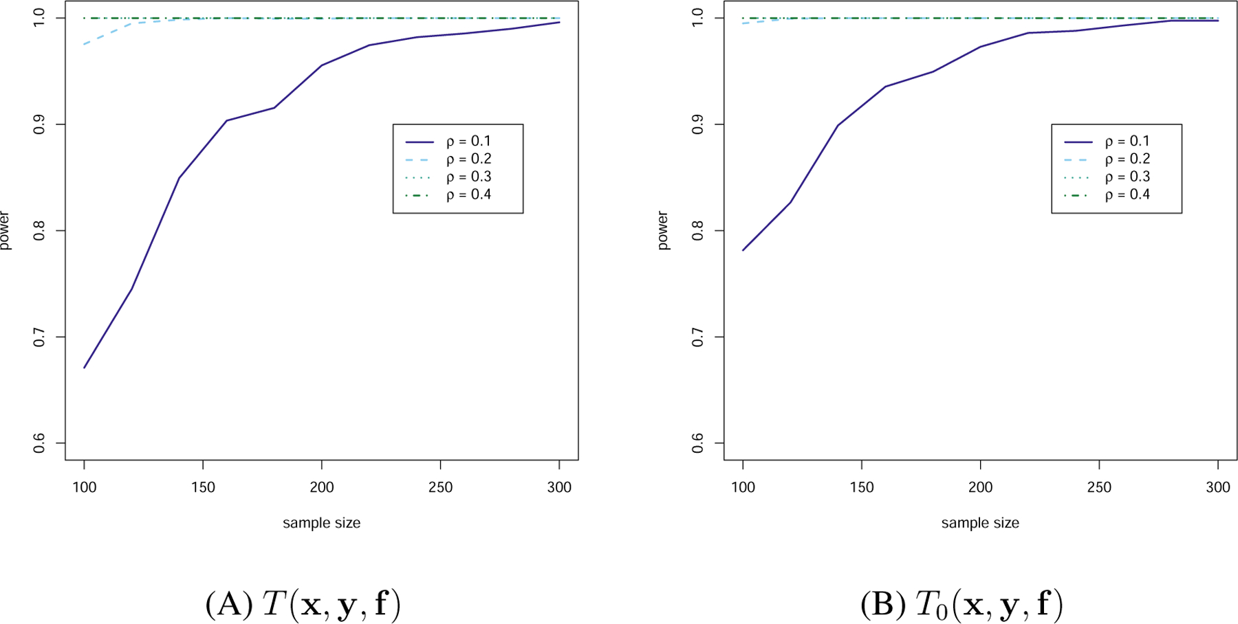
Power-sample size graph of Example 1

From Figure 1, it is clear that as the sample size or ρ increases, the empirical power also increases in general. Also, comparing the panels (A) and (B) in Figure 1, we see that when the sample size is small, the P-DCov test has smaller power than the oracle test, however, the difference between them becomes negligible as the sample size increases. This is consistent with our theory regarding the asymptotic distribution of the test statistics. When ρ = 0, Table 1 reports the empirical type I error for both P-DCov as well as the oracle version. It is clear that the type I error of P-DCov is under good control as the sample size increases.

Table 1:

Type I error of Example 1

Test based on ${\widehat{\mathit{ϵ}}}_x$ and ${\widehat{\mathit{ϵ}}}_y$
n	100	120	140	160	180	200	220	240	260	280	300
	0.119	0.114	0.116	0.100	0.098	0.097	0.092	0.102	0.094	0.091	0.096
Test based on ϵx and ϵy
n	100	120	140	160	180	200	220	240	260	280	300
	0.086	0.102	0.104	0.094	0.092	0.091	0.096	0.103	0.098	0.092	0.095

Example 4.2. [Gaussian graphical model] We consider a Gaussian graphical model with precision matrix Ω = Σ⁻¹, where Ω is a tridiagonal matrix of size d × d, and is associated with the autoregressive process of order one. We set d = 100 and the (i, j)-element in Σ to be σ_i,j = exp(−|s_i − s_j|), where $0=s_1<s_2<\cdots <s_d$. In addition,

$$s_i-s_{i-1}\stackrel{i.i.d}{~}Uniform\left(1,3\right),\hspace{1em}i=2,\dots ,d.$$

In this example, we would like to compare the proposed P-DCov with the state-of-the-art approaches for recovering Gaussian graphical models. In terms of recovering structure Ω, we compare lasso.dcov (projection by lasso followed by distance covariance), sam.dcov (projection by sparse additive model followed by distance covariance), lasso.pearson (projection by lasso followed by Pearson correlation), sam.pearson (projection by sparse additive model followed by Pearson correlation) with three popular estimators corresponding to the lasso, adaptive lasso and scad penalized likelihoods (called graphical.lasso, graphical.alasso and graphical.scad on the graph) for the precision matrix (Friedman et al., 2008; Fan et al., 2009). Here, lasso.dcov and sam.dcov are two examples of our P-DCov methods. We use R package SAM to fit the sparse additive model. To evaluate the performances, we construct receiver operating characteristic (ROC) curves for each method with sample sizes n = 100 and n = 300. The process of constructing the ROC curves involves conducting the P-DCov test for each pair of nodes and record the corresponding P-values. In each of the ROC curve, true positive rates (TPR) are plotted against false positive rates (FPR) at various thresholds of those P-values (“TP” means the true entry of the precision matrix is nonzero and estimated as nonzero; “FP” means the true entry of the precision matrix is zero but estimated as nonzero). We follow the implementation in Fan et al. (2009) for the three penalized likelihood estimators. The average results over 100 replications of different methods are reported in Figure 2. The associated AUC (Area Under the Curve) for each method is also displayed in the legend of the figure.

Figure 2:

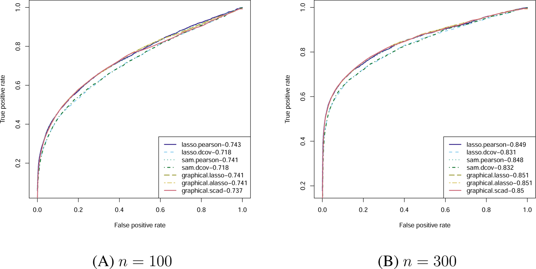
ROC curves for Gaussian graphical models with AUCs in legends.

We observe that lasso.pearson and sam.pearson perform similarly to the penalized likelihood methods when n = 100. On the other hand, lasso.dcov and sam.dcov lead to slightly smaller AUC value due to the use of the distance covariance, which is expected for the Gaussian model. This shows that we do not pay a big price for using the more complicated distance covariance and sparse additive model.

Example 4.3. [A general graphical model] We consider a general graphical model with a combination of multivariate t distribution and multivariate Gaussian distribution. The dimension of x is d = 100. In detail, $\text{x}={\left({\text{x}}_1^T,{\text{x}}_2^T,{\text{x}}_3^T\right)}^T$ where x₁ follows a 20 dimensional multivariate t distribution with degrees of freedom 5, location parameter 0 and identity covariance matrix, x₂ follows the same Gaussian graphical model as in Example 4.2 except the dimension is now 10, and ${\text{x}}_3~\mathcal{N}\left(0,{\text{I}}_{70}\right)$. In addition, x₁, x₂, and x₃ are mutually independent.

To generate a multivariate t-distribution, we first generate a random vector w₂₀ from the standard multivariate Gaussian distribution and an independent random variable $\tau ~{\chi }^2\left(5\right)$ and then set ${\text{x}}_1=\text{w}/\sqrt{\tau }$. One important fact about the multivariate t distribution is that the zero element in the precision matrix does not imply conditional independence like the case of Gaussian graphical models (Finegold and Drton, 2009). Indeed, for x₁, we actually have the fact that ${\text{x}}_1^{\left(i\right)}$ and ${\text{x}}_1^{\left(j\right)}$ are dependent given ${\text{x}}_1^{\left(-i,-j\right)}$ for any pair 1 ≤ i ≠ j ≤ 20. On the contrary, the Gaussian likelihood based methods will falsely claim that all the components of x₁ are independent, because the corresponding elements in Ω are 0.

The average ROC curve results are rendered in Figure 3. As expected, by using the new projection based distance covariance method for testing conditional independence, lasso.dcov outperforms all the other methods in terms of AUC, with a more evident advantage when n = 300. One interesting observation is that: in the region where FPR is very low, the likelihood based methods actually outperform P-DCov methods. One possible reason is that the likelihood based methods are more capable of capturing the conditional dependency structure within x₂ as it follows a Gaussian graphical model.

Figure 3:

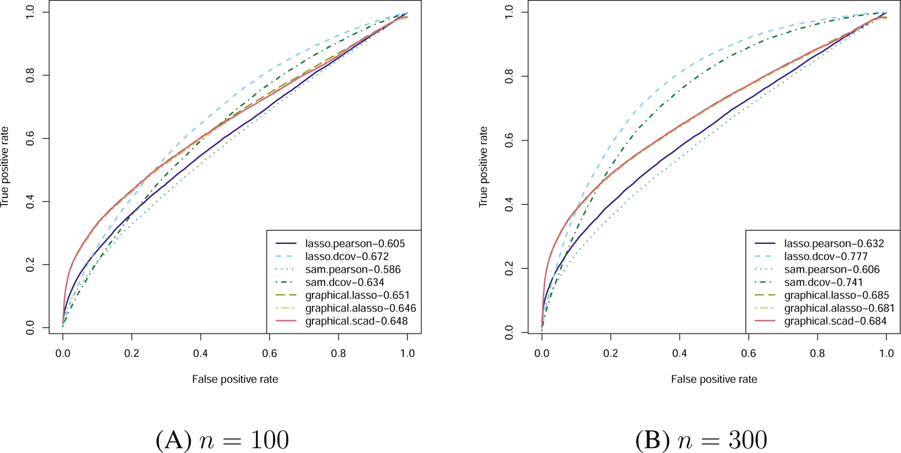
ROC curves for a general graphical model with AUCs in legends.

Example 4.4. [Dependency graph with external factors] We consider a dependency graph with the contribution of external factors. In particular, we generate $\text{u}~\mathcal{N}\left(0,\text{Ω}\right)$, where Ω is the same tridiagonal matrix used in Example 4.2 except the dimension is now 30 and $\mathbf{\text{f}}~\mathcal{N}\left(0,{\mathbf{\text{I}}}_{300}\right)$, then the observation x = u + Qg(f) where Q_30×300 is a sparse coefficient matrix that dictates how each dimension of x depends on the factor g(f). In particular, we let $\text{Q}=\left[{\tilde{\text{Q}}}_{30\times 15},0_{30\times 285}\right]$ with the generation of $\widetilde{\mathbf{\text{Q}}}$ follows the setting in Cai et al. (2013). For each element ${\tilde{Q}}_{ij}$, we first generate a Bernoulli distribution with success probability 0.2 to determine whether ${\tilde{Q}}_{ij}$ is 0 or not. If ${\tilde{Q}}_{ij}$ is not 0, we then generate ${\tilde{Q}}_{ij}~Uniform\left(0.5,1\right)$. Here we consider two forms of g(·), namely g(f) = f and g(f) = f².

Now, we report results regarding the average ROC curves for lasso.pearson, lasso.dcov, sam.pearson and sam.dcov. The results for both g(f) = f and g(f) = f² are depicted in Figure 4. Note that we are not building a conditional dependency graph among x, but a dependency graph of x conditioning on the external factor f. There are some insightful observations from the figure. First of all, by looking at the first case when g(f) = f, it is clear that lasso.pearson is the best as it takes advantage of the sparse linear structure paired with the Gaussian distribution of the residual. By using the distance covariance as a dependency measure, or by using the sparse additive model as a projection method, it is reassuring that we do not lose much efficiency. Second, for the case when g(f) = f² and n = 300, we can see a substantial advantage of the sparse additive model based methods as they can capture this nonlinear contribution of the factors to the dependency structure of x.

Figure 4:

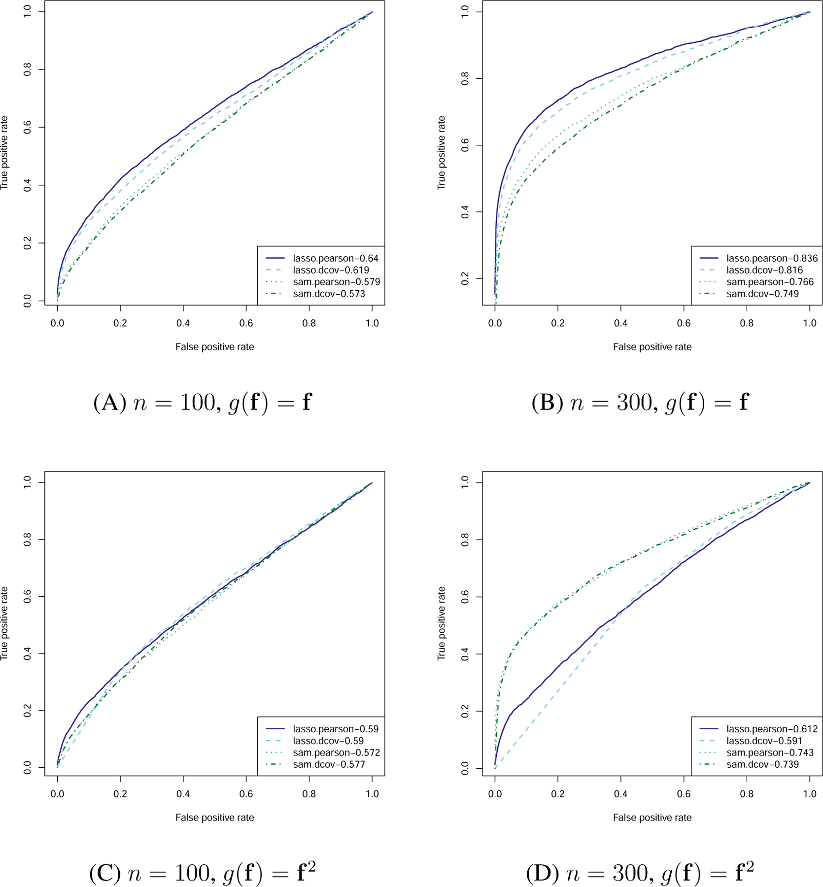
ROC curves for factor based dependency graph with AUCs in legends.

Example 4.5. [A general graphical model with external factors] We consider a general conditional dependency graph with the contribution of external factors by combining the ingredients of Examples 4.3 and 4.4. In particular, we generate $\mathbf{\text{u}}=\left({\mathbf{\text{x}}}_1^T,{\mathbf{\text{x}}}_2^T\right)$ with x₁ and x₂ generated from Example 4.3 and $\mathbf{\text{f}}~\mathcal{N}\left(0,{\mathbf{\text{I}}}_{300}\right)$, then set x = u + Qg(f) where Q is the same as Example 4.4. We also consider g(f) = f and g(f) = f².

In this example, we would like to investigate the performance of a two-step projection method. In particular, we first project x onto the space spanned by f and denote the residual by $\widehat{\mathbf{\text{u}}}$. Then we explore the conditional dependency structure of ${\widehat{\mathbf{\text{u}}}}^{\left(i\right)}$ and ${\widehat{\mathbf{\text{u}}}}^{\left(j\right)}$ given ${\widehat{\mathbf{\text{u}}}}^{\left(-i,-j\right)}$ by projecting them onto the space orthogonal to the space (linearly or additively) spanned by ${\widehat{\mathbf{\text{u}}}}^{\left(-i,-j\right)}$. Here, we compare the performances of methods using the external factor and those that ignore them. The average ROC curves are rendered in Figure 5.

Figure 5:

ROC curves for a general graphical model with external factors (AUCs in legends).

From Figure 5, we see that first of all, when g(f) = f, the methods using external factors outperform their counterparts without using the information with the best method being lasso.dcov. Second, when we have nonlinear factors, using the factors do not necessarily help when we only consider linear projection. For example, the performances of lasso.pearson and lasso.pearson.f in panel (c) illustrates this point. On the other hand, by using sparse additive model based projection, we have a substantial gain over all the remaining methods especially for n = 300.

5. Real Data Analysis

We collect daily excess returns of 90 stocks among the S&P 100 index, which are available between August 19, 2004 and August 19, 2005. We chose the starting date as Google’s Initial Public Offering date, and consider one year of daily excess returns since then. In particular, we consider the following Fama-French three factors model (Fama and French, 1993)

$$r_{it}-r_{ft}={\beta }_{i,\text{MKT}}\left({\text{MKT}}_t-r_{ft}\right)+{\beta }_{i,\text{SMB}}{\text{SMB}}_t+{\beta }_{i,\text{HML}}{\text{HML}}_t+u_{it},$$

for i = 1, …, 90 and t = 1, …, 252. At time t, r_it represents the return for stock i, r_ft is the risk-free rate, and MKT_t, SMB_t and HML_t constitute market, size and value factors, respectively.

5.1. Individual stocks

In the first experiment, we study the conditional dependency on all pairs of stocks, with the conditioning set being the Fama-French three factors in Section 5.1.1. Then, we further add the industry factor to the conditioning set in Section 5.1.2.

5.1.1. Fama-French three-factors effect

We perform P-DCov test with FDR control on all pairs of stocks and study the dependence between stocks conditioning on the Fama-French three factors. Under significance level α = 0.01, we found out that 15.46% of the pairs of stocks are conditionally dependent given the three factors, which implies that the three factors may not be sufficient to explain the dependencies among stocks. As a comparison, we also implemented the conditional independence test with the distance covariance based test replaced by Pearson correlation based test. It turns out the 9.34% of the pairs are significant under the same significance level. This shows the P-DCov test is more powerful than the Pearson correlation test in discovering significant pairs that are conditionally dependent.

We then investigate the top 5 pairs of stocks that correspond to the largest test statistic values using the P-DCov test. They are (BHI, SLB), (CVX, XOM), (HAL, SLB), (COP, CVX), and (BHI, HAL). Interestingly, all six stocks involved are closely related to the oil industry. This reveals the high level of dependence among oil industry stocks that cannot be well explained by the Fama-French three factors model. In addition, we examine the stock pairs that are conditionally dependent under the P-DCov test but not under the Pearson correlation test. The two most significant pairs are (C, USB) and (MRK, PFE). The first pair is in the financial industry (Citigroup and U.S. Bancorp) and the second pair is pharmaceutical companies (Merck & Co. and Pfizer). This shows that by using the proposed P-DCov, some interesting conditional dependency structures could be recovered. This is consistent with the findings that the within-sector correlations are still present even after adjusting for Fama-French factors and 10 industrial factors (Fan et al., 2016).

5.1.2. Industry factor effect

For the top 5 stock pairs with the largest test statistics after conditioning on the Fama-French three factors in Section 5.1.1, we would like to evaluate how much of the conditional dependency comes from the industry group effect. In particular, as these stocks all come from the energy industry, we computed the corresponding test statistics before and after further conditioning on the energy group (XLE), in addition to the Fama-French three factors. We summarized the results in Table 2, where columns “woXLE (stat)” and “wXLE (stat)” contain values of the test statistic before and after further conditioning on XLE respectively for each pair. The columns “woXLE (p-value)” and “wXLE (p-value)” contain the corresponding p-values. From the table, we first see that after conditioning on XLE in additional to the Fama-French three factors, all five stock pairs become less dependent with much smaller test statistic values, which agrees with intuition since we remove the impact of industry factor with the additional conditioning. A second observation is that, while the five pairs of stocks are listed in decreasing order in terms of distance covariance before conditioning on the industry factor (in columns containing “woXLE”), the order of these pairs changed after conditioning (in columns containing “wXLE”). This implies that the industry effects may play quite different roles for these pairs of stocks, when we evaluate distance covariances. After carefully investigating the five pairs, we found that CVX, XOM, and COP are oil companies which are directly impacted by XLE, whereas BHI, SLB, and HAL are energy service companies. This may explain that compared with (CVX, XOM) and (COP, CVX), (BHI, SLB), (HAL, SLB) and (BHI, HAL) have a relatively larger test statistic after conditioning on the industry factor XLE in additional to the Fama-French three factors. Some other possible issues that may affect the conditional dependency include the liquidity of stocks (Haugen and Baker, 1996).

Table 2:

The conditional independence test statistics and their associated p-values before and after conditioning on the energy group effect (XLE) for the 5 pairs of stocks.

Stock Pair	woXLE (stat)	woXLE (p-value)	wXLE (stat)	wXLE (p-value)
(BHI, SLB)	46.92	1e–6	15.09	1e–6
(CVX, XOM)	35.71	1e–6	1.86	0.043
(HAL, SLB)	34.81	1e–6	5.19	2.7e–5
(COP, CVX)	34.12	1e–6	1.00	0.389
(BHI, HAL)	33.67	1e–6	6.41	2e–6

5.2. Stock groups by industry

One advantage of our proposed procedure is that P-DCov can investigate dependence between two multivariate vectors, not necessarily of the same dimension, conditioning on external factors. As an illustration, beyond studying the relationship of stocks within industrial sectors as in Section 5.1.1, we explore dependency structures between industrial sectors conditioning on the Fama-French three factors. In particular, we group the stocks in S&P 100 into 32 industrial groups based on the “Sectoring by industry groups” information provided on https://www.nasdaq.com. Each of the industrial group now contains a few stocks, with a full list provided in Table 6 in Appendix. We perform P-DCov test on all pairs of industrial groups conditioning on the same Fama-French three factors in Section 5.1.1. Table 3 presents the pairs of industrial groups (containing more than 2 stocks) which attain the smallest P-value of 1e-6, and for readers’ convenience, we list the stocks corresponding to each selected groups in Table 4. A few interesting findings are the following. Industry ‘Conglomerates’ (containing stocks of General Electric, Honeywell, 3M and United Technologies Corporation), is conditionally dependent of both ‘Aerospace’ (containing stocks of Boeing, General Dynamics and Raytheon) and ‘Transportation’ (containing stocks of FedEx, Norfolk Southern and UPS-United Parcel Service). A plausible explanation is that the companies in sector ‘Conglomerates’ may produce supplies such as components/gadgets for sector ‘Aerospace’ and ‘Transportation’ and therefore the returns of these industrial sectors might be dependent. Similarly, ‘Large Cap Pharma’ (containing stocks of Bristol-Myers Squibb, Johnson & Johnson, Merck & Co and Pfizer) is conditionally dependent of ‘Medical Products’ (containing stocks of Abbott Laboratories, Baxter International and Medtronic) and ‘Soap and Cleaning Products’ (containing stocks of Colgate-Palmolive and Procter & Gamble). The first relationship can be explained as Pharmaceutical versus Health care and the second is due to the fact that companies in ‘Soap and Cleaning Products’ are big suppliers of the Pharmaceutical companies in terms of their commonly used commodities. Lastly, based on the industrial division provided by Nasdaq, sector ‘Finance’ contains mainly investment banks while sector ‘Banks’ contains the usual regional and commercial banks. It is reasonable to believe these two sectors are closely dependent. The rest of the pairs are detected as significant although we cannot provide an obvious explanation. Nevertheless, since the Fama-French three factors are conditioned out, the discovered conditional dependencies can be subtle. We will leave them to experts for further investigation.

Table 6:

The industry groups and their associated stocks.

Metal Products	AA
Medical	AMGN
Steel	ATI
Cosmetics & Toiletries	AVP
Medical Products	ABT BAX MDT
Utility	AEP AES ETR EXC SO
Insurance	AIG ALL CI HIG
Finance	AXP COF GS MS
Aerospace	BA GD RTN
Banks	BAC C JPM RF USB WFC
Large Cap Pharma	BMY JNJ MRK PFE
Beverages	CCU KO
Machinery	CAT
Soap and Cleaning Products	CL PG
Cable TV	CMCSA
Oil	COP CVX HAL SLB WMB XOM
Food	CPB
Computer	CSCO HPQ IBM MSFT ORCL PEP
Media Conglomerates	DIS
Auto	F
Transportation	FDX NSC UPS
Conglomerates	GE HON MMM UTX
Internet	GOOG
Building Prds Retail	HD
Semi General	INTC TXN
Paper & Related Products	IP
Retail	MCD TGT WMT
Tobacco	MO
Industrial Robotics	ROK
Wireless National	S T VZ
Building Products	WY
Business Services	XRX

Table 3:

Pairs of stock groups with the smallest P-value 1e–6.

Conglomerates	Aerospace
Large Cap Pharma	Medical Products
Soap and Cleaning Products	Large Cap Pharma
Conglomerates	Transportation
Banks	Finance
Banks	Medical Products
Conglomerates	Banks
Banks	Utility
Soap and Cleaning Products	Banks
Wireless National	Banks

Table 4:

The stocks corresponding to each selected industry.

Banks	BAC C JPM RF USB WFC
Large Cap Pharma	BMY JNJ MRK PFE
Soap and Cleaning Products	CL PG
Conglomerates	GE HON MMM UTX
Wireless National	S T VZ
Medical Products	ABT BAX MDT
Utility	AEP AES ETR EXC SO
Finance	AXP COF GS MS
Aerospace	BA GD RTN
Transportation	FDX NSC UPS

After looking at the interesting pairs corresponding to the smallest P-values, we apply FDR control with α = 0.01 and selected 27 important pairs with results presented in Tables 5 and 6. Similar messages can be discovered and we leave out the detailed discussions due to the large number of pairs.

Table 5:

The selected important pairs of industry groups with FDR control under α = 0.01.

Banks	Medical Products
Banks	Utility
Banks	Medical
Banks	Finance
Large Cap Pharma	Medical Products
Large Cap Pharma	Medical
Soap and Cleaning Products	Cosmetics & Toiletries
Soap and Cleaning Products	Banks
Soap and Cleaning Products	Large Cap Pharma
Conglomerates	Aerospace
Conglomerates	Banks
Conglomerates	Transportation
Retail	Building Prds Retail
Wireless National	Banks
Building Products	Paper & Related Products
Banks	Insurance
Building Products	Conglomerates
Conglomerates	Utility
Conglomerates	Machinery
Paper & Related Products	Conglomerates
Building Products	Transportation
Large Cap Pharma	Banks
Business Services	Computer
Soap and Cleaning Products	Medical Products
Semi General	Computer
Conglomerates	Medical Products
Paper & Related Products	Metal Products

6. Discussion

In this work, we proposed a general framework for testing conditional independence via projection and showed a new way to create dependency graphs. A few future directions worth exploration. Firstly, the current theoretical results assume that contribution of factors is sparse linear. How to extend the theory to the case of sparse additive model projection would be an interesting future work. The second potential direction is to extend the methodology and theory to the case where the dimensions of x and y grow with n.

Furthermore, the proposed methodology could be generalised to test the conditional independency of multiple random vectors {X₁, …, X_N} given a common factor f by taking advantage of a recent result by Böttcher et al. (2019), which developed a new dependency measure for multiple random vectors. A preliminary description of the extension is as follows.

1. Estimate the errors $\left\{{\mathit{ϵ}}_{X_j},j=1,\cdots ,N\right\}$ by the projection methods described in the current paper. Denote the corresponding estimates as $\left\{{\widehat{\mathit{ϵ}}}_{X_j},j=1,\cdots ,N\right\}$.

2. With a predetermined significance level α, we reject the null hypothesis if the normalized total multivariance (see Test B in Section 4.5 of Böttcher et al. (2019) for details) satisfies

   $${N\cdot \hspace{0.17em}}^N{\overline{\mathcal{M}}}_p^2\left({\widehat{\mathit{ϵ}}}_{X_1},\cdots ,{\widehat{\mathit{ϵ}}}_{X_N}\right)\ge {\chi }_{1-\alpha }^2\left(1\right),$$

   where ${ }^N{\overline{\mathcal{M}}}_p^2(\cdot )$ is the normalized total multivariance function specified in definition 4.17 in Böttcher et al. (2019).

The detailed impact of the estimated error on the asymptotic distribution of the test statistic is worth further investigation.

An R package pgraph for implementing the proposed methodology is available on CRAN.

Appendix

Lemma 3. Under Condition 3, we have ${\text{max}}_{i,j}\Vert ({\mathbf{\text{B}}}_x-{\widehat{\mathbf{\text{B}}}}_x)\left({\mathbf{\text{f}}}_i-{\mathbf{\text{f}}}_j\right)\Vert =O_P\left(a_n\right)$ and $\mathbb{E}{\text{max}}_{i,j}\Vert ({\mathbf{\text{B}}}_x-{\widehat{\mathbf{\text{B}}}}_x)\left({\mathbf{\text{f}}}_i-{\mathbf{\text{f}}}_j\right)\Vert =O\left(a_n\right)$.

Proof. From Condition 3, it is obvious that ${\text{max}}_{i,j}\Vert ({\mathbf{\text{B}}}_x-{\widehat{\mathbf{\text{B}}}}_x)\left({\mathbf{\text{f}}}_i-{\mathbf{\text{f}}}_j\right)\Vert =O_P\left(a_n\right)$. Let $U_n={\text{max}}_{i,j}\Vert ({\mathbf{\text{B}}}_x-{\widehat{\mathbf{\text{B}}}}_x)\left({\mathbf{\text{f}}}_i-{\mathbf{\text{f}}}_j\right)\Vert$ and ${\tilde{U}}_n=U_n/a_n$. Then, we have

$$\begin{gathered} \mathbb{E}\left({\tilde{U}}_n\right)={\int }_0^{\infty }\mathbb{P}\left({\tilde{U}}_n>t\right)dt \\ ={\int }_0^1\mathbb{P}\left({\tilde{U}}_n>t\right)dt+{\int }_0^{\infty }\mathbb{P}\left({\tilde{U}}_n>t\right)dt \\ \le 1+{\int }_0^{\infty }{C}_1^{-t}dt<\infty . \end{gathered}$$

As a result, the lemma is proved.□

For the remaining proofs, we apply Taylor expansion to $\Vert {\widehat{\mathit{ϵ}}}_{i,x}-{\widehat{\mathit{ϵ}}}_{j,x}\Vert$ at ${\mathit{ϵ}}_{i,x}-{\mathit{ϵ}}_{j,x}$ and get

$$\begin{gathered} \Vert {\widehat{\mathit{ϵ}}}_{i,x}-{\widehat{\mathit{ϵ}}}_{j,x}\Vert =\Vert {\mathit{ϵ}}_{i,x}-{\mathit{ϵ}}_{j,x}\Vert +\frac{{\text{c}}_{i,j,x}^{\top }}{\Vert {\text{c}}_{i,j,x}\Vert }({\mathbf{\text{B}}}_x-{\widehat{\mathbf{\text{B}}}}_x\mathbf{)}\left({\mathbf{\text{f}}}_i-{\mathbf{\text{f}}}_j\right)=\Vert {\mathit{ϵ}}_{i,x}-{\mathit{ϵ}}_{j,x}\Vert +D_{i,j,x}, \\ \Vert {\widehat{\mathit{ϵ}}}_{i,y}-{\widehat{\mathit{ϵ}}}_{j,y}\Vert =\Vert {\mathit{ϵ}}_{i,y}-{\mathit{ϵ}}_{j,y}\Vert +\frac{{\text{c}}_{i,j,y}^{\top }}{\Vert {\text{c}}_{i,j,y}\Vert }\mathbf{\left(}{\mathbf{\text{B}}}_y-{\widehat{\mathbf{\text{B}}}}_y\mathbf{\right)}\left({\mathbf{\text{f}}}_i-{\mathbf{\text{f}}}_j\right)=\Vert {\mathit{ϵ}}_{i,y}-{\mathit{ϵ}}_{j,y}\Vert +D_{i,j,y}, \end{gathered}$$ (13)

where ${\text{c}}_{i,j,x}={\lambda }_{i,j,x}\left({\widehat{\mathit{ϵ}}}_{i,x}-{\widehat{\mathit{ϵ}}}_{j,x}\right)+\left(1-{\lambda }_{i,j,x}\right)\left({\mathit{ϵ}}_{i,x}-{\mathit{ϵ}}_{j,x}\right)$ and ${\text{c}}_{i,j,y}={\lambda }_{i,j,y}\left({\widehat{\mathit{ϵ}}}_{i,y}-{\widehat{\mathit{ϵ}}}_{j,y}\right)+\left(1-{\lambda }_{i,j,y}\right)\left({\mathit{ϵ}}_{i,y}-{\mathit{ϵ}}_{j,y}\right)$, for ${\lambda }_{i,j,x}\in \left[0,1\right]$ and ${\lambda }_{i,j,y}\in \left[0,1\right]$.

of Theorem 1. Using the Taylor expansion in (13), we have the following decomposition

$${\mathcal{V}}_n^2\left({\widehat{\mathit{ϵ}}}_x,{\widehat{\mathit{ϵ}}}_y\right)\_{\mathcal{V}}_n^2\left({\mathit{ϵ}}_x,{\mathit{ϵ}}_y\right)=T_1+T_2+T_3,$$

where

$$T_1=\frac{1}{n^2}\sum _{i,j=1}^n{D}_{i,j,x}\Vert {\mathit{ϵ}}_{i,y}-{\mathit{ϵ}}_{j,y}\Vert +\frac{1}{n^2}\sum _{i,j=1}^n{D}_{i,j,x}\frac{1}{n^2}\sum _{k,l=1}^n\Vert {\mathit{ϵ}}_{k,y}-{\mathit{ϵ}}_{l,y}\Vert -\frac{2}{n^3}\sum _{i=1}^n\sum _{j,k=1}^n{D}_{i,j,x}\Vert {\mathit{ϵ}}_{i,y}-{\mathit{ϵ}}_{k,y}\Vert ,$$ (14)

$$T_2=\frac{1}{n^2}\sum _{i,j=1}^n{D}_{i,j,y}\Vert {\mathit{ϵ}}_{i,x}-{\mathit{ϵ}}_{j,x}\Vert +\frac{1}{n^2}\sum _{i,j=1}^n{D}_{i,j,y}\frac{1}{n^2}\sum _{k,l=1}^n\Vert {\mathit{ϵ}}_{k,x}-{\mathit{ϵ}}_{l,x}\Vert -\frac{2}{n^3}\sum _{i=1}^n\sum _{j,k=1}^n{D}_{i,j,y}\Vert {\mathit{ϵ}}_{i,x}-{\mathit{ϵ}}_{k,x}\Vert ,$$ (15)

$$T_3=\frac{1}{n^2}\sum _{i,j=1}^n{D}_{i,j,x}{D}_{i,j,y}+\frac{1}{n^2}\sum _{i,j=1}^n{D}_{i,j,x}\frac{1}{n^2}\sum _{i,j=1}^n{D}_{i,j,y}-\frac{2}{n^3}\sum _{i=1}^n\sum _{j,k=1}^n{D}_{i,j,x}{D}_{i,k,y}.$$ (16)

By Condition 3, we have ${\text{max}}_{i,j}\left|D_{i,j,x}\right|\le 2{\Vert ({\mathbf{\text{B}}}_x-{\widehat{\mathbf{\text{B}}}}_x)\mathbf{\text{f}}\Vert }_{2,\infty }\le O_p\left(a_n\right)$. Therefore,

$$\left|T_1\right|=O_p\left(a_n\right)\left(\frac{4}{n^2}\sum _{i,j=1}^n\Vert {\mathit{ϵ}}_{i,y}-{\mathit{ϵ}}_{j,y}\Vert \right),$$

$$\left|T_2\right|=O_p\left(a_n\right)\left(\frac{4}{n^2}\sum _{i,j=1}^n\Vert {\mathit{ϵ}}_{i,x}-{\mathit{ϵ}}_{j,x}\Vert \right),$$

$$\left|T_3\right|=O_p\left(a_n^2\right).$$

Another fact we easily observe is that: $n^{-2}{\sum }_{i,j=1}^n\Vert {\mathit{ϵ}}_{i,x}-{\mathit{ϵ}}_{j,x}\Vert =O_p\left(1\right)$, since $\mathbb{E}\Vert {\mathit{ϵ}}_{i,x}-{\mathit{ϵ}}_{j,x}\Vert$ is uniformly bounded over all (i, j) pairs and so is $\mathbb{E}(n^{-2}{\sum }_{i,j=1}^n\Vert {\mathit{ϵ}}_{i,x}-{\mathit{ϵ}}_{j,x}\Vert )$.

As a result, we know ${\mathcal{V}}_n^2\left({\widehat{\mathit{ϵ}}}_x,{\widehat{\mathit{ϵ}}}_y\right)-{\mathcal{V}}_n^2\left({\mathit{ϵ}}_x,{\mathit{ϵ}}_y\right)\stackrel{P}{\to }0$. This combined with Lemma 1 leads to

$${\mathcal{V}}_n^2\left({\widehat{\mathit{ϵ}}}_x,{\widehat{\mathit{ϵ}}}_y\right)\stackrel{P}{\to }{\mathcal{V}}^2\left({\mathit{ϵ}}_x,{\mathit{ϵ}}_y\right).$$

□

Remark: The result of Theorem 1 cannot be implied from that of Theorem 2, since independence between ϵ_x and ϵ_y is not assumed.

Lemma 4. For the c_i,j,x and c_i,j,y defined in (13), we have the following approximation error bound on the normalized version.

$$\Vert \frac{{\text{c}}_{i,j,x}}{\Vert {\text{c}}_{i,j,x}\Vert }-\frac{{\mathit{ϵ}}_{i,x}-{\mathit{ϵ}}_{j,x}}{\Vert {\mathit{ϵ}}_{i,x}-{\mathit{ϵ}}_{j,x}\Vert }\Vert \le \frac{2}{\Vert {\mathit{ϵ}}_{i,x}-{\mathit{ϵ}}_{j,x}\Vert }\underset{i,j}{\text{max}}\Vert ({\mathbf{\text{B}}}_x-{\widehat{\mathbf{\text{B}}}}_x)\left({\mathbf{\text{f}}}_i-{\mathbf{\text{f}}}_j\right)\Vert ,$$ (17)

$$\Vert \frac{{\text{c}}_{i,j,y}}{\Vert {\text{c}}_{i,j,y}\Vert }-\frac{{\mathit{ϵ}}_{i,y}-{\mathit{ϵ}}_{j,y}}{\Vert {\mathit{ϵ}}_{i,y}-{\mathit{ϵ}}_{j,y}\Vert }\Vert \le \frac{2}{\Vert {\mathit{ϵ}}_{i,y}-{\mathit{ϵ}}_{j,y}\Vert }\underset{i,j}{\text{max}}\Vert \mathbf{\left(}{\mathbf{\text{B}}}_y-{\widehat{\mathbf{\text{B}}}}_y\mathbf{\right)}\left({\mathbf{\text{f}}}_i-{\mathbf{\text{f}}}_j\right)\Vert .$$ (18)

Proof. It suffices to show (17). First, we will show

$$\Vert \frac{{\text{c}}_{i,j,x}}{\Vert {\text{c}}_{i,j,x}\Vert }-\frac{{\mathit{ϵ}}_{i,x}-{\mathit{ϵ}}_{j,x}}{\Vert {\mathit{ϵ}}_{i,x}-{\mathit{ϵ}}_{j,x}\Vert }\Vert \le \Vert \frac{{\widehat{\mathit{ϵ}}}_{i,x}-{\widehat{\mathit{ϵ}}}_{j,x}}{\Vert {\widehat{\mathit{ϵ}}}_{i,x}-{\widehat{\mathit{ϵ}}}_{j,x}\Vert }-\frac{{\mathit{ϵ}}_{i,x}-{\mathit{ϵ}}_{j,x}}{\Vert {\mathit{ϵ}}_{i,x}-{\mathit{ϵ}}_{j,x}\Vert }\Vert .$$ (19)

Denote by α₁ and α₂ the angle between c_i,j,x and ϵ_i,x−ϵ_j,x, and the angle between ${\widehat{\mathit{ϵ}}}_{i,x}-{\widehat{\mathit{ϵ}}}_{j,x}$ and ϵ_i,x − ϵ_j,x, respectively. It is easy to see that 0 ≤ α₁ ≤ α₂ ≤ π, and hence cos α₁ ≥ cos α₂. By cosine formula,

$${\Vert \frac{{\text{c}}_{i,j,x}}{\Vert {\text{c}}_{i,j,x}\Vert }-\frac{{\mathit{ϵ}}_{i,x}-{\mathit{ϵ}}_{j,x}}{\Vert {\mathit{ϵ}}_{i,x}-{\mathit{ϵ}}_{j,x}\Vert }\Vert }^2=2-2\hspace{0.17em}\text{cos}\hspace{0.17em}{\alpha }_1,\hspace{0.17em}\hspace{0.17em}\hspace{0.17em}\text{and}\hspace{0.17em}\hspace{0.17em}{\Vert \frac{{\widehat{\mathit{ϵ}}}_{i,x}-{\widehat{\mathit{ϵ}}}_{j,x}}{\Vert {\widehat{\mathit{ϵ}}}_{i,x}-{\widehat{\mathit{ϵ}}}_{j,x}\Vert }-\frac{{\mathit{ϵ}}_{i,x}-{\mathit{ϵ}}_{j,x}}{\Vert {\mathit{ϵ}}_{i,x}-{\mathit{ϵ}}_{j,x}\Vert }\Vert }^2=2-2\hspace{0.17em}\text{cos}\hspace{0.17em}{\alpha }_2.$$

Therefore, (19) is proved and it remains to show that

$$\Vert \frac{{\widehat{\mathit{ϵ}}}_{i,x}-{\widehat{\mathit{ϵ}}}_{j,x}}{\Vert {\widehat{\mathit{ϵ}}}_{i,x}-{\widehat{\mathit{ϵ}}}_{j,x}\Vert }-\frac{{\mathit{ϵ}}_{i,x}-{\mathit{ϵ}}_{j,x}}{\Vert {\mathit{ϵ}}_{i,x}-{\mathit{ϵ}}_{j,x}\Vert }\Vert \le \frac{2}{\Vert {\mathit{ϵ}}_{i,x}-{\mathit{ϵ}}_{j,x}\Vert }\underset{i,j,\in \left\{1,\dots ,n\right\}}{\text{max}}\Vert ({\mathbf{\text{B}}}_x-{\widehat{\mathbf{\text{B}}}}_x)\left({\mathbf{\text{f}}}_i-{\mathbf{\text{f}}}_j\right)\Vert .$$ (20)

Left hand side of (20) can be rewritten as

$$\begin{gathered} \Vert \frac{{\widehat{\mathit{ϵ}}}_{i,x}-{\widehat{\mathit{ϵ}}}_{j,x}}{\Vert {\widehat{\mathit{ϵ}}}_{i,x}-{\widehat{\mathit{ϵ}}}_{j,x}\Vert }-\frac{{\mathit{ϵ}}_{i,x}-{\mathit{ϵ}}_{j,x}}{\Vert {\mathit{ϵ}}_{i,x}-{\mathit{ϵ}}_{j,x}\Vert }\Vert \\ =\Vert \frac{\left[\left({\widehat{\mathit{ϵ}}}_{i,x}-{\widehat{\mathit{ϵ}}}_{j,x}\right)-\left({\mathit{ϵ}}_{i,x}-{\mathit{ϵ}}_{j,x}\right)\right]\Vert {\widehat{\mathit{ϵ}}}_{i,x}-{\widehat{\mathit{ϵ}}}_{j,x}\Vert -\left(\Vert {\widehat{\mathit{ϵ}}}_{i,x}-{\widehat{\mathit{ϵ}}}_{j,x}\Vert -\Vert {\mathit{ϵ}}_{i,x}-{\mathit{ϵ}}_{j,x}\Vert \right)\left({\widehat{\mathit{ϵ}}}_{i,x}-{\widehat{\mathit{ϵ}}}_{j,x}\right)}{\Vert {\widehat{\mathit{ϵ}}}_{i,x}-{\widehat{\mathit{ϵ}}}_{j,x}\Vert \Vert {\mathit{ϵ}}_{i,x}-{\mathit{ϵ}}_{j,x}\Vert }\Vert \\ \le \frac{1}{\Vert {\mathit{ϵ}}_{i,x}-{\mathit{ϵ}}_{j,x}\Vert }\left(\Vert \left({\widehat{\mathit{ϵ}}}_{i,x}-{\widehat{\mathit{ϵ}}}_{j,x}\right)-\left({\mathit{ϵ}}_{i,x}-{\mathit{ϵ}}_{j,x}\right)\Vert +\left|\Vert {\widehat{\mathit{ϵ}}}_{i,x}-{\widehat{\mathit{ϵ}}}_{j,x}\Vert -\Vert {\mathit{ϵ}}_{i,x}-{\mathit{ϵ}}_{j,x}\Vert \right|\right) \\ \le \frac{2}{\Vert {\mathit{ϵ}}_{i,x}-{\mathit{ϵ}}_{j,x}\Vert }\underset{i,j\in \left\{1,\dots ,n\right\}}{\text{max}}\Vert ({\mathbf{\text{B}}}_x-{\widehat{\mathbf{\text{B}}}}_x)\left({\mathbf{\text{f}}}_i-{\mathbf{\text{f}}}_j\right)\Vert . \end{gathered}$$

Combining (19) and (20), the lemma is proved. □

Lemma 5. Under Conditions 1 and 2, and the null hypothesis that ${\mathit{ϵ}}_x\hspace{0.17em}⫫{\mathit{ϵ}}_y$, for any γ > 0,

$$\frac{1}{n^{\gamma }\text{log}\hspace{0.17em}n}\left[\frac{1}{n^2}\sum _{i,j=1}^n\frac{1}{\Vert {\mathit{ϵ}}_{i,x}-{\mathit{ϵ}}_{j,x}\Vert }\right]\stackrel{P}{\to }0,\hspace{0.17em}\frac{1}{n^{\gamma }\text{log}\hspace{0.17em}n}\left[\frac{1}{n^2}\sum _{i,j=1}^n\frac{1}{\Vert {\mathit{ϵ}}_{i,y}-{\mathit{ϵ}}_{j,y}\Vert }\right]\stackrel{P}{\to }0.$$

Proof. We will only show the first result involving ϵ_x with the other one follows similarly. For any δ > 0, let

$$R_n=\frac{1}{n^2}\sum _{i,j=1}^n\frac{1}{\Vert {\mathit{ϵ}}_{i,x}-{\mathit{ϵ}}_{j,x}\Vert },\hspace{1em}{\overline{R}}_n=\frac{1}{n^2}\sum _{i,j=1}^n\left[\frac{1}{\Vert {\mathit{ϵ}}_{i,x}-{\mathit{ϵ}}_{j,x}\Vert }\wedge n^{2+\delta }\right].$$

Then for ∀ ϵ > 0,

$$\mathbb{P}\left[\left|R_n-{\overline{R}}_n\right|>\mathit{ϵ}\right]\le n^2\mathbb{P}\left[\Vert {\mathit{ϵ}}_{i,x}-{\mathit{ϵ}}_{j,x}\Vert <n^{-2-\delta }\right]\le C{n}^2{n}^{-2-\delta }=C{n}^{-\delta },$$ (21)

due to the Condition 2 that the density function of ‖ϵ_i,x − ϵ_j,x‖ is pointwise bounded.

Therefore, $\left|R_n-{\overline{R}}_n\right|\stackrel{P}{\to }0$, which leads to

$$\left|\frac{R_n}{n^{\gamma }\text{log}\hspace{0.17em}n}-\frac{{\overline{R}}_n}{n^{\gamma }\text{log}\hspace{0.17em}n}\right|\stackrel{P}{\to }0.$$ (22)

On the other hand,

$$\begin{gathered} \hspace{1em}\mathbb{E}\left[\frac{1}{\text{log}\hspace{0.17em}n}\frac{1}{\Vert {\mathit{ϵ}}_{i,x}-{\mathit{ϵ}}_{j,x}\Vert }\wedge n^{2+\delta }\right] \\ =\frac{1}{\text{log}\hspace{0.17em}n}\mathbb{P}\left(\frac{1}{\Vert {\mathit{ϵ}}_{i,x}-{\mathit{ϵ}}_{j,x}\Vert }>n^{2+\delta }\right)n^{2+\delta }+\frac{1}{\text{log}\hspace{0.17em}n}{\int }_{n^{-2-\delta }}^{\infty }\frac{1}{t}{h}_{\Vert {\mathit{ϵ}}_{i,x}-{\mathit{ϵ}}_{j,x}\Vert }\left(t\right)dt \\ \le \frac{C}{\text{log}\hspace{0.17em}n}+\frac{1}{\text{log}\hspace{0.17em}n}{\int }_{n^{-2-\delta }}^{C_0}\frac{1}{x}{h}_{\Vert {\mathit{ϵ}}_{i,x}-{\mathit{ϵ}}_{j,x}\Vert }\left(x\right)dx+\frac{1}{\text{log}\hspace{0.17em}n}{\int }_{C_0}^{\infty }\frac{1}{t}{h}_{\Vert {\mathit{ϵ}}_{i,x}-{\mathit{ϵ}}_{j,x}\Vert }\left(t\right)dt \\ \le \frac{C}{\text{log}\hspace{0.17em}n}+\frac{C}{\text{log}\hspace{0.17em}n}{\int }_{n^{-2-\delta }}^{C_0}\frac{1}{x}dx+\frac{1}{C_0\text{log}\hspace{0.17em}n}\mathbb{P}\left(\Vert {\mathit{ϵ}}_{i,x}-{\mathit{ϵ}}_{j,x}\Vert >C_0\right) \\ \le \frac{C}{\text{log}\hspace{0.17em}n}+\frac{C}{\text{log}\hspace{0.17em}n}\left[\text{log}\left(C_0\right)+\text{log}\left(n^{2+\delta }\right)\right]+\frac{1}{C_0\text{log}\hspace{0.17em}n} \\ \le \frac{C}{\text{log}\hspace{0.17em}n}+C^{\prime }+\frac{1}{C_0\text{log}\hspace{0.17em}n}, \end{gathered}$$ (23)

where $h_{\Vert {\mathit{ϵ}}_{i,x}-{\mathit{ϵ}}_{j,x}\Vert }$ is the density of ‖ϵ_i,x − ϵ_j,x‖. In the above derivation, the first inequality can be easily seen from (21) and the second inequality utilizes Condition 2.

Therefore, ${\overline{R}}_n/\text{log}\hspace{0.17em}n$ is bounded in L₁ and since n^γ → ∞, ${\overline{R}}_n/\left[n^{\gamma }\text{log}\left(n\right)\right]$ converges to 0 in L₁ and hence in probability, i.e.,

$$\frac{{\overline{R}}_n}{n^{\gamma }\text{log}\left(n\right)}\stackrel{P}{\to }0.$$ (24)

This, combined with (22) yields

$$\frac{R_n}{n^{\gamma }\text{log}\left(n\right)}\stackrel{P}{\to }0.$$ (25)

This completes the proof of Lemma 5. □

To prove Theorem 2, we first introduce two propositions.

Proposition 1. Under Conditions 1 and 2, and the null hypothesis that ${\mathit{ϵ}}_x\hspace{0.17em}⫫{\mathit{ϵ}}_y$,

$$T_1=O_p\left(a_n/n\right),\hspace{0.17em}{T}_2=O_p\left(a_n/n\right)$$

Proof. From (14), we rewrite T₁ as

$$\begin{gathered} T_1=\frac{1}{n^2}\sum _{i,j=1}^n{D}_{i,j,x}\left(\Vert {\mathit{ϵ}}_{i,y}-{\mathit{ϵ}}_{j,y}\Vert +\frac{1}{n^2}\sum _{k,l=1}^n\Vert {\mathit{ϵ}}_{k,y}-{\mathit{ϵ}}_{l,y}\Vert -\frac{1}{n}\sum _{k=1}^n\Vert {\mathit{ϵ}}_{i,y}-{\mathit{ϵ}}_{k,y}\Vert -\frac{1}{n}\sum _{k=1}^n\Vert {\mathit{ϵ}}_{j,y}-{\mathit{ϵ}}_{k,y}\Vert \right) \\ \hspace{1em}\doteq \frac{1}{n^2}\sum _{i,j=1}^n{D}_{i,j,x}{A}_{i,j,y}, \end{gathered}$$

with A_i,j,y self-defined by the equation.

Let us consider term

$$\mathbb{E}\left(T_1^2\right)=\frac{1}{n^4}\sum _{i\ne j,k\ne l}\mathbb{E}\left(D_{i,j,x}{D}_{k,l,x}{A}_{i,j,y}{A}_{k,l,y}\right)=\frac{1}{n^4}\sum _{i\ne j,k\ne l}\mathbb{E}\left(D_{i,j,x}{D}_{k,l,x}\right)\mathbb{E}\left(A_{i,j,y}{A}_{k,l,y}\right).$$ (26)

We can separate the above quantity into three parts. It is easy to see that D_i,j,x are identically distributed with respect to different pairs of (i, j) when i ≠ j. Let us define the following three sets of index quadruples:

• I₁ = {(i, j, k, l)|there are four distinct values in {i, j, k, l}}.

• I₂ = {(i, j, k, l)|i ≠ j, k ≠ l, and there are three distinct values in {i, j, k, l}}.

• I₃ = {(i, j, k, l)|i ≠ j, k ≠ l, and there are two distinct values in {i, j, k, l}}.

Let us suppose $\mathbb{E}\left(D_{i,j,x}{D}_{k,l,x}\right)=c_1$, for (i, j, k, l) ∈ I₁;$\mathbb{E}\left(D_{i,j,x}{D}_{k,l,x}\right)=c_2$, for (i, j, k, l) ∈ I₂.$\mathbb{E}\left(D_{i,j,x}{D}_{k,l,x}\right)=c_3$, for (i, j, k, l) ∈ I₃. By Condition 3, we know c₁, c₂ and c₃ are all of order $O\left(a_n^2\right)$. Also, $\mathbb{E}\left(A_{i,j,y}\right)=O\left(1\right)$. Then we have

$$\mathbb{E}\left(T_1^2\right)=\mathbb{E}\left(\frac{c_1}{n^4}\sum _{I_1}{A}_{i,j,y}{A}_{k,l,y}+\frac{c_2}{n^4}\sum _{I_2}{A}_{i,j,y}{A}_{k,l,y}+\frac{c_3}{n^4}\sum _{I_3}{A}_{i,j,y}{A}_{k,l,y}\right).$$ (27)

On the other hand, we observe that ${\sum }_{j=1}^n{A}_{i,j,y}=0$ by definition and A_i,j,y = A_j,i,y, so we have

$$\sum _{I_2}{A}_{i,j,y}{A}_{k,l,y}=\sum _{i=1}^n{(\sum _{j=1}^n{A}_{i,j,y})}^2-\sum _{i=1}^n\sum _{j=1}^n{A}_{i,j,y}^2=-\sum _{i=1}^n\sum _{j=1}^n{A}_{i,j,y}^2.$$

By Condition 1, we know all the second order terms of distances of differences (‖ϵ_i,y − ϵ_j,y‖², ‖ϵ_i,y−ϵ_j,y‖·‖ϵ_i,y−ϵ_k,y‖ as examples) have bounded expectation, and thus all the second order terms of A_i,j,y’s also have bounded expectations. Therefore, $\mathbb{E}(n^{-4}{\sum }_{I_3}{A}_{i,j,y}{A}_{k,l,y})=O\left(n^{-2}\right)$. Finally, since ${\sum }_{i=1}^n{\sum }_{j=1}^n{A}_{i,j,y}=0$,

$$\begin{gathered} \sum _{I_1}{A}_{i,j,y}{A}_{k,l,y}={(\sum _{i=1}^n\sum _{j=1}^n{A}_{i,j,y})}^2-\sum _{I_2}{A}_{i,j,y}{A}_{k,l,y}-\sum _{I_3}{A}_{i,j,y}{A}_{k,l,y}-\sum _{i=1}^n{A}_{i,i,y}^2 \\ =-\sum _{I_2}{A}_{i,j,y}{A}_{k,l,y}-\sum _{I_3}{A}_{i,j,y}{A}_{k,l,y}-\sum _{i=1}^n{A}_{i,i,y}^2. \end{gathered}$$

This combined with our previous calculations leads to $\mathbb{E}(n^{-4}{\sum }_{I_1}{A}_{i,j,y}{A}_{k,l,y})=O\left(n^{-2}\right)$. As a result, we have $\mathbb{E}\left(T_1^2\right)=O\left(a_n^2/n^2\right)$. Together with Chebychev’s inequality, we know $T_1^2=O_p\left(a_n^2/n^2\right)$ and equivalently, T₁ = O_p(a_n/n). Similarly, we could show that T₂ = O_p(a_n/n). □

Proposition 2. Under Conditions 1, 2, 3, and 4, and the null hypothesis that ${\mathit{ϵ}}_x\hspace{0.17em}⫫{\mathit{ϵ}}_y$,

$$T_3=O_p\left\{\left(n^{-1/2}{a}_n^2\right)\vee \left(a_n^3\left(\text{log}\hspace{0.17em}n\right)n^{\gamma }\right)\vee \left(n^{-1/2}{a}_n{e}_n\text{log}\hspace{0.17em}K\right)\right\}.$$

Proof. Recall that

$$\begin{gathered} T_3=\frac{1}{n^2}\sum _{i,j=1}^n{D}_{i,j,x}{D}_{i,j,y}+\frac{1}{n^2}\sum _{i,j=1}^n{D}_{i,j,x}\frac{1}{n^2}\sum _{i,j=1}^n{D}_{i,j,y}-\frac{2}{n^3}\sum _{i=1}^n\sum _{j,k=1}^n{D}_{i,j,x}{D}_{i,k,y} \\ \doteq \frac{1}{n^2}\sum _{i,j=1}^n{D}_{i,j,x}{B}_{i,j,y}, \end{gathered}$$

with B_i,j,y self-defined in the above equation. We can easily see that ${\sum }_{i=1}^n{B}_{i,j,y}=0$, for any j. Let B_max = max_i,j |B_i,j,y|, then we define ${\tilde{B}}_{i,j,y}=B_{i,j,y}/\left(2B_{\text{max}}\right)+0.5$. In this way, we know ${\tilde{B}}_{i,j,y}\in \left[0,1\right]$ and ${\sum }_{i=1}^n{\tilde{B}}_{i,j,y}=1/2$ for any j. By Condition 3, we know that B_max = O_p(a_n). Also, since all ${\tilde{B}}_{i,j,y}$ are non-negative, by Cauchy-Schwartz, we can upper bound ${\Vert \tilde{\text{B}}\Vert }_F$ with the case when ${\tilde{B}}_{i,j,y}$ have the same values across i. Thus, ${\Vert \tilde{\text{B}}\Vert }_F=O_p\left(\sqrt{n}\right)$.

Then we can rewrite T₃ in the following form:

$$T_3=\frac{2B_{\text{max}}}{n^2}\sum _{i,j=1}^n{D}_{i,j,x}{\tilde{B}}_{i,j,y}-\frac{B_{\text{max}}}{n^2}\sum _{i,j=1}^n{D}_{i,j,x}\doteq T_{31}-T_{32}.$$

Let us look at T₃₁ first. If we denote D and $\tilde{\text{B}}$ as the matrix of dimension n × n composed of elements D_i,j,x and ${\tilde{B}}_{i,j,y}$, we know that

$$\left|T_{31}\right|\le \frac{2B_{\text{max}}}{n^2}{\Vert \text{D}\Vert }_F{\Vert \tilde{\text{B}}\Vert }_F=O_p\left(a_n/n^2\right)O_p\left(a_{n}n\right)O_p\left(\sqrt{n}\right)=O_p\left(\frac{a_n^2}{\sqrt{n}}\right).$$ (28)

Then, let us proceed to term T₃₂. Here, we write D_i,j,x in another form as a sum of two terms and bound them separately.

$$\begin{gathered} D_{i,j,x}=\frac{{\left({\mathit{ϵ}}_{i,x}-{\mathit{ϵ}}_{j,x}\right)}^{\top }}{\Vert {\mathit{ϵ}}_{i,x}-{\mathit{ϵ}}_{j,x}\Vert }({\mathbf{\text{B}}}_x-{\widehat{\mathbf{\text{B}}}}_x)\left({\mathbf{\text{f}}}_i-{\mathbf{\text{f}}}_j\right)+\left(\frac{{\text{c}}_{i,j,x}}{\Vert {\text{c}}_{i,j,x}\Vert }-\frac{\left({\mathit{ϵ}}_{i,x}-{\mathit{ϵ}}_{j,x}\right)}{\Vert {\mathit{ϵ}}_{i,x}-{\mathit{ϵ}}_{j,x}\Vert }\right)({\mathbf{\text{B}}}_x-{\widehat{\mathbf{\text{B}}}}_x)\left({\mathbf{\text{f}}}_i-{\mathbf{\text{f}}}_j\right) \\ \equiv \frac{{\left({\mathit{ϵ}}_{i,x}-{\mathit{ϵ}}_{j,x}\right)}^{\top }}{\Vert {\mathit{ϵ}}_{i,x}-{\mathit{ϵ}}_{j,x}\Vert }({\mathbf{\text{B}}}_x-{\widehat{\mathbf{\text{B}}}}_x)\left({\mathbf{\text{f}}}_i-{\mathbf{\text{f}}}_j\right)+r_{i,j,x}. \end{gathered}$$ (29)

As a result, we know

$$T_{32}=\frac{B_{\text{max}}}{n^2}\sum _{i,j=1}^n{r}_{i,j,x}+\frac{B_{\text{max}}}{n^2}\sum _{i,j=1}^n\frac{{\left({\mathit{ϵ}}_{i,x}-{\mathit{ϵ}}_{j,x}\right)}^{\top }}{\Vert {\mathit{ϵ}}_{i,x}-{\mathit{ϵ}}_{j,x}\Vert }({\mathbf{\text{B}}}_x-{\widehat{\mathbf{\text{B}}}}_x)\left({\mathbf{\text{f}}}_i-{\mathbf{\text{f}}}_j\right).$$

By Lemma 4, we know

$$\left|r_{i,j,x}\right|\le \underset{i,j}{\text{max}}{\Vert ({\mathbf{\text{B}}}_x-{\widehat{\mathbf{\text{B}}}}_x)\left({\mathbf{\text{f}}}_i-{\mathbf{\text{f}}}_j\right)\Vert }^2\frac{2}{\Vert {\mathit{ϵ}}_{i,x}-{\mathit{ϵ}}_{j,x}\Vert },$$ (30)

where ${\text{max}}_{i,j}{\Vert \left({\mathbf{\text{B}}}_x-{\widehat{\mathbf{\text{B}}}}_x\right)\left({\mathbf{\text{f}}}_i-{\mathbf{\text{f}}}_j\right)\Vert }^2=O_p\left(a_n^2\right)$.

Together with Lemma 5, the first term in T₃₂ has rate

$$n^{-2}{B}_{\text{max}}\sum _{i,j=1}^n{r}_{i,j,x}=O_p\left(a_n^3\left(\text{log}\hspace{0.17em}n\right)n^{\gamma }\right).$$

The second term in T₃₂ can be rewritten in terms of trace:

$$\hspace{1em}\Vert \frac{B_{\text{max}}}{n^2}\sum _{i,j=1}^n\frac{{\left({\mathit{ϵ}}_{i,x}-{\mathit{ϵ}}_{j,x}\right)}^{\top }}{\Vert {\mathit{ϵ}}_{i,x}-{\mathit{ϵ}}_{j,x}\Vert }({\mathbf{\text{B}}}_x-{\widehat{\mathbf{\text{B}}}}_x)\left({\mathbf{\text{f}}}_i-{\mathbf{\text{f}}}_j\right)\Vert$$ (31)

$$\begin{gathered} =\left|B_{\text{max}}\text{Tr}\left(({\mathbf{\text{B}}}_x-{\widehat{\mathbf{\text{B}}}}_x)\frac{1}{n^2}\sum _{i,j=1}^n\left({\mathbf{\text{f}}}_i-{\mathbf{\text{f}}}_j\right)\frac{{\left({ϵ}_{i,x}-{ϵ}_{j,x}\right)}^{\top }}{\Vert {ϵ}_{i,x}-{ϵ}_{j,x}\Vert }\right)\right|, \\ \doteq \left|B_{\text{max}}\text{Tr}\left(\left({\mathbf{\text{B}}}_x-{\widehat{\mathbf{\text{B}}}}_x\right)\text{W}\right)\right|, \\ \le B_{\text{max}}\sum _{l=1}^p{\Vert B_{x,l}-{\widehat{B}}_{x,l}\Vert }_1\underset{i,j}{\text{max}}\left|W\left(i,j\right)\right|, \end{gathered}$$ (32)

where W is self-defined and W (i, j) is the element on the i-th row and j-column of matrix W. Let us take (i, j) = (1, 1) as an example, and look at $W\left(1,1\right)=\frac{1}{n^2}{\sum }_{i,j=1}^n\left(f_{i,1}-f_{j,1}\right)\frac{{\mathit{ϵ}}_{i,x,1}-{\mathit{ϵ}}_{j,x,1}}{\Vert {\mathit{ϵ}}_{i,x}-{\mathit{ϵ}}_{j,x}\Vert }$. We easily see that $\mathbb{E}W\left(1,1\right)=0$, due to facts: and ϵ_i,x and ϵ_i,x are mutually independent of f with any observation indices; and $\mathbb{E}\left[\left({\mathit{ϵ}}_{i,x}-{\mathit{ϵ}}_{j,x}\right)/\Vert {\mathit{ϵ}}_{i,x}-{\mathit{ϵ}}_{j,x}\Vert \right]=0$. Furthermore,

$$\mathbb{E}(W{\left(1,1\right)}^2)=\frac{1}{n^4}\sum _{i,j,k,l=1}^n\left(f_{i,1}-f_{j,1}\right)\frac{{\mathit{ϵ}}_{i,x,1}-{\mathit{ϵ}}_{j,k,1}}{\Vert {\mathit{ϵ}}_{i,x}-{\mathit{ϵ}}_{j,x}\Vert }\left(f_{k,1}-f_{l,1}\right)\frac{{\mathit{ϵ}}_{k,x,1}-{\mathit{ϵ}}_{l,k,1}}{\Vert {\mathit{ϵ}}_{k,x}-{\mathit{ϵ}}_{l,x}\Vert }.$$

Similar to the reasoning in Proposition 1, we have n⁴ terms in I₁. But in this scenario, $\mathbb{E}\left(f_{i,1}-f_{j,1}\right)\frac{{\mathit{ϵ}}_{i,x,1}-{\mathit{ϵ}}_{j,x,1}}{\Vert {\mathit{ϵ}}_{i,x}-{\mathit{ϵ}}_{j,x}\Vert }\left(f_{k,1}-f_{l,1}\right)\frac{{\mathit{ϵ}}_{k,x,1}-{\mathit{ϵ}}_{l,x,1}}{\Vert {\mathit{ϵ}}_{k,x}-{\mathit{ϵ}}_{l,x}\Vert }=0$ due to independence, therefore we know

$$\mathbb{E}\left(W{\left(1,1\right)}^2\right)=O\left(1/n\right).$$

As a result, we know |W (1, 1)| = O_p(n^−1/2), and thus max_i,j |W (i, j)| = O_p(n^−1/2 log K). Furthermore, we can bound the term in (31) with rate O_p(n^−1/2a_ne_n log K).

Combining T₃₁ and T₃₂, we know $T_3=O_p\left\{\left(n^{-1/2}{a}_n^2\right)\vee \left(a_n^3\left(\text{log}\hspace{0.17em}n\right)n^{\gamma }\right)\vee \left(n^{-1/2}{a}_n{e}_n\text{log}\hspace{0.17em}K\right)\right\}$. □

Proof of Theorem 2. Recall the notations we used in the proof of Theorem 1,

$${\mathcal{V}}_n^2\left({\widehat{ϵ}}_x,{\widehat{ϵ}}_y\right)-{\mathcal{V}}_n^2\left({ϵ}_x,{ϵ}_y\right)=T_1+T_2+T_3.$$

By Propositions 1 and 2, Conditions 3 and 4, we have for any γ > 0,

$$n\left(T_1+T_2+T_3\right)=O_p\left(a_n\right)+O_p\left\{\left(a_n^2\sqrt{n}\right)\vee \left(n^{1+\gamma }\left(\text{log}\hspace{0.17em}n\right)a_n^3\right)\vee \left(a_n{e}_n\text{log}\hspace{0.17em}K\sqrt{n}\right)\right\}=o_p\left(1\right).$$

Combined with Lemma 2, the theorem is proved. □

Proof of Corollary 2. The result follows directly from the proofs of Theorems 1 and 2 and an application of Slutsky’s theorem. □

Proof of Theorem 3. The proof of Theorem 3 follows similarly as Theorem 6 in Székely et al. (2007). Here we omit the details for brevity. □

References

- Anderson TW, 1962. An introduction to multivariate statistical analysis. Wiley; New York. [Google Scholar]
- Belloni A, Chernozhukov V, 2011. L1-penalized quantile regression in high-dimensional sparse models. The Annals of Statistics 39, 82–130. [Google Scholar]
- Belloni A, Chernozhukov V, Wang L, 2011. Square-root lasso: pivotal recovery of sparse signals via conic programming. Biometrika 98, 791–806. [Google Scholar]
- Belloni A, Chernozhukov V, et al. , 2013. Least squares after model selection in high-dimensional sparse models. Bernoulli 19, 521–547. [Google Scholar]
- Benjamini Y, Hochberg Y, 1995. Controlling the false discovery rate: a practical and powerful approach to multiple testing. Journal of the Royal Statistical Society. Series B (Methodological), 289–300.
- Blomqvist N, 1950. On a measure of dependence between two random variables. The Annals of Mathematical Statistics, 593–600.
- Blum J, Kiefer J, Rosenblatt M, 1961. Distribution free tests of independence based on the sample distribution function. The Annals of Mathematical Statistics, 485–498.
- Böttcher B, Keller-Ressel M, Schilling RL, 2019. Distance multivariance: New dependence measures for random vectors. The Annals of Statistics 47, 2757–2789. [Google Scholar]
- Bühlmann P, Van De Geer S, 2011. Statistics for high-dimensional data: methods, theory and applications. Springer Science & Business Media.
- Cai T, Liu W, Luo X, 2011. A constrained L1 minimization approach to sparse precision matrix estimation. Journal of the American Statistical Association 106, 594–607. [Google Scholar]
- Cai TT, Li H, Liu W, Xie J, 2013. Covariate-adjusted precision matrix estimation with an application in genetical genomics. Biometrika 100, 139–156. [DOI] [PMC free article] [PubMed] [Google Scholar]
- Chen S, Witten DM, Shojaie A, 2014. Selection and estimation for mixed graphical models. Biometrika 102, 47–64. [DOI] [PMC free article] [PubMed] [Google Scholar]
- Dempster AP, 1972. Covariance selection. Biometrics, 157–175.
- Drton M, Perlman MD, 2004. Model selection for gaussian concentration graphs. Biometrika 91, 591–602. [Google Scholar]
- Edwards D, 2000. Introduction to graphical modelling. Springer. [Google Scholar]
- Fama EF, French KR, 1993. Common risk factors in the returns on stocks and bonds. Journal of Financial Economics 33, 3–56. [Google Scholar]
- Fan J, 1992. Design-adaptive nonparametric regression. Journal of the American statistical Association 87, 998–1004. [Google Scholar]
- Fan J, Feng Y, Song R, 2011. Nonparametric independence screening in sparse ultra-high dimensional additive models. Journal of the American Statistical Association 106, 544–557. [DOI] [PMC free article] [PubMed] [Google Scholar]
- Fan J, Feng Y, Wu Y, 2009. Network exploration via the adaptive lasso and scad penalties. The Annals of Applied Statistics 3, 521. [DOI] [PMC free article] [PubMed] [Google Scholar]
- Fan J, Furger A, Xiu D, 2016. Incorporating global industrial classification standard into portfolio allocation: A simple factor-based large covariance matrix estimator with high frequency data. Journal of Business & Economic Statistics, 489–503.
- Fan J, Ke Y, Sun Q, Zhou WX, 2018. Farm-test: Factor-adjusted robust multiple testing with false discovery control. Journal of American Statistical Association, to appear. [DOI] [PMC free article] [PubMed]
- Fan J, Li Q, Wang Y, 2017. Robust estimation of high-dimensional mean regression. Journal of the Royal Statistical Society: Series B (Statistical Methodology) 79, 247–265. [DOI] [PMC free article] [PubMed] [Google Scholar]
- Finegold MA, Drton M, 2009. Robust graphical modeling with t-distributions, in: Proceedings of the Twenty-Fifth Conference on Uncertainty in Artificial Intelligence, AUAI Press; pp. 169–176. [Google Scholar]
- Friedman J, Hastie T, Tibshirani R, 2008. Sparse inverse covariance estimation with the graphical lasso. Biostatistics 9, 432–441. [DOI] [PMC free article] [PubMed] [Google Scholar]
- Van de Geer S, Bühlmann P, Ritov Y, Dezeure R, et al. , 2014. On asymptotically optimal confidence regions and tests for high-dimensional models. The Annals of Statistics 42, 1166–1202. [Google Scholar]
- Gretton A, Bousquet O, Smola A, Schölkopf B, 2005. Measuring statistical dependence with hilbert-schmidt norms, in: International conference on algorithmic learning theory, Springer; pp. 63–77. [Google Scholar]
- Hastie T, Tibshirani R, Wainwright M, 2015. Statistical learning with sparsity: the lasso and generalizations. CRC Press. [Google Scholar]
- Haugen RA, Baker NL, 1996. Commonality in the determinants of expected stock returns. Journal of Financial Economics 41, 401–439. [Google Scholar]
- Heller R, Heller Y, Gorfine M, 2012. A consistent multivariate test of association based on ranks of distances. Biometrika 100, 503–510. [Google Scholar]
- Hoeffding W, 1948. A non-parametric test of independence. The Annals of Mathematical Statistics, 546–557.
- Hollander M, Wolfe DA, Chicken E, 2013. Nonparametric statistical methods. John Wiley & Sons. [Google Scholar]
- Huo X, Székely GJ, 2016. Fast computing for distance covariance. Technometrics 58, 435–447. [Google Scholar]
- Jankova J, Van De Geer S, 2015. Confidence intervals for high-dimensional inverse covariance estimation. Electronic Journal of Statistics 9, 1205–1229. [Google Scholar]
- Lauritzen SL, 1996. Graphical models. Oxford University Press. [Google Scholar]
- Linton O, Gozalo P, 1997. Conditional independence restrictions: testing and estimation. V Cowles Foundation Discussion Paper 1140. [Google Scholar]
- Liu W, 2013. Gaussian graphical model estimation with false discovery rate control. The Annals of Statistics 41, 2948–2978. [Google Scholar]
- Meinshausen N, Bühlmann P, 2006. High-dimensional graphs and variable selection with the lasso. The Annals of Statistics, 1436–1462.
- Ravikumar P, Lafferty J, Liu H, Wasserman L, 2009. Sparse additive models. Journal of the Royal Statistical Society: Series B (Statistical Methodology) 71, 1009–1030. [Google Scholar]
- Ren Z, Sun T, Zhang CH, Zhou HH, 2015. Asymptotic normality and optimalities in estimation of large gaussian graphical models. The Annals of Statistics 43, 991–1026. [Google Scholar]
- Rigby R, Stasinopoulos D, 1996. A semi-parametric additive model for variance heterogeneity. Statistics and Computing 6, 57–65. [Google Scholar]
- Rigby RA, Stasinopoulos DM, 2005. Generalized additive models for location, scale and shape. Journal of the Royal Statistical Society: Series C (Applied Statistics) 54, 507–554. [Google Scholar]
- Sen A, Sen B, 2014. Testing independence and goodness-of-fit in linear models. Biometrika 101, 927–942. [Google Scholar]
- Stock JH, Watson MW, 2002. Macroeconomic forecasting using diffusion indexes. Journal of Business & Economic Statistics 20, 147–162. [Google Scholar]
- Stone CJ, 1985. Additive regression and other nonparametric models. The Annals of Statistics 13, 689–705. [Google Scholar]
- Su L, White H, 2007. A consistent characteristic function-based test for conditional independence. Journal of Econometrics 141, 807–834. [Google Scholar]
- Su L, White H, 2008. A nonparametric hellinger metric test for conditional independence. Econometric Theory 24, 829–864. [Google Scholar]
- Su L, White H, 2014. Testing conditional independence via empirical likelihood. Journal of Econometrics 182, 27–44. [Google Scholar]
- Székely GJ, Rizzo ML, Bakirov NK, 2007. Measuring and testing dependence by correlation of distances. The Annals of Statistics 35, 2769–2794. [Google Scholar]
- Voorman A, Shojaie A, Witten D, 2013. Graph estimation with joint additive models. Biometrika 101, 85–101. [DOI] [PMC free article] [PubMed] [Google Scholar]
- Wainwright MJ, Jordan MI, 2008. Graphical models, exponential families, and variational inference. Foundations and Trends® in Machine Learning 1, 1–305. [Google Scholar]
- Wang L, 2013. The l1 penalized lad estimator for high dimensional linear regression. Journal of Multivariate Analysis 120, 135–151. [Google Scholar]
- Wang X, Pan W, Hu W, Tian Y, Zhang H, 2015. Conditional distance correlation. Journal of the American Statistical Association 110, 1726–1734. [DOI] [PMC free article] [PubMed] [Google Scholar]
- Wilks S, 1935. On the independence of k sets of normally distributed statistical variables. Econometrica, Journal of the Econometric Society, 309–326.
- Yu G, Bien J, 2017. Learning local dependence in ordered data. Journal of Machine Learning Research 18, 1–60. [Google Scholar]
- Zhang CH, Zhang SS, 2014. Confidence intervals for low dimensional parameters in high dimensional linear models. Journal of the Royal Statistical Society: Series B (Statistical Methodology) 76, 217–242. [Google Scholar]